On the Benefits of Sampling in Privacy Preserving Statistical Analysis on Distributed Databases

Abstract

We consider a problem where mutually untrusting curators possess portions of a vertically partitioned database containing information about a set of individuals. The goal is to enable an authorized party to obtain aggregate (statistical) information from the database while protecting the privacy of the individuals, which we formalize using Differential Privacy. This process can be facilitated by an untrusted server that provides storage and processing services but should not learn anything about the database. This work describes a data release mechanism that employs Post Randomization (PRAM), encryption and random sampling to maintain privacy, while allowing the authorized party to conduct an accurate statistical analysis of the data. Encryption ensures that the storage server obtains no information about the database, while PRAM and sampling ensures individual privacy is maintained against the authorized party. We characterize how much the composition of random sampling with PRAM increases the differential privacy of system compared to using PRAM alone. We also analyze the statistical utility of our system, by bounding the estimation error — the expected $\ell_{2}$-norm error between the true empirical distribution and the estimated distribution — as a function of the number of samples, PRAM noise, and other system parameters. Our analysis shows a tradeoff between increasing PRAM noise versus decreasing the number of samples to maintain a desired level of privacy, and we determine the optimal number of samples that balances this tradeoff and maximizes the utility. In experimental simulations with the UCI “Adult Data Set” and with synthetically generated data, we confirm that the theoretically predicted optimal number of samples indeed achieves close to the minimal empirical error, and that our analytical error bounds match well with the empirical results.

I Introduction

One of the most visible technological trends is the emergence and proliferation of large-scale data collection. Public and private enterprises are collecting tremendous volumes of data on individuals, their activities, their preferences, their locations, their medical histories, and so on. These enterprises include government organizations, healthcare providers, financial institutions, internet search engines, social networks, cloud service providers, and many other kinds of private companies. Naturally, interested parties could potentially discern meaningful patterns and gain valuable insights if they were able to access and correlate the information across these large, distributed databases. For example, a social scientist may want to determine the correlations between individual income with personal characteristics such as gender, race, age, education, etc., or a medical researcher may want to study the relationships between disease prevalence and individual environmental factors. In such applications, it is imperative to maintain the privacy of individuals, while ensuring that the useful aggregate (statistical) information is only revealed to the authorized parties. Indeed, unless the public is satisfied that their privacy is being preserved, they would not provide their consent for the collection and use of their personal information. Additionally, the inherent distribution of this data across multiple curators present a significant challenge, as privacy concerns and policy would likely prevent these curators from directly sharing their data to facilitate statistical analysis in a centralized fashion. Thus, tools must be developed for conducting statistical analysis on large and distributed databases, while addressing these privacy and policy concerns.

As an example, consider two curators Alice and Bob, who possess two databases containing census-type information about individuals in a population, as shown in Figure 1. Suppose that this data is to be combined and made available to authorized researchers studying salaries in the population, while ensuring that the privacy of the individual respondents is maintained. Conceptually, a data release mechanism involves the “sanitization” of the data (via some form of perturbation or transform) to preserve individual privacy, before making it available for data analysis. The suitability of the method used to sanitize the data is determined by the extent to which rigorously defined privacy constraints are met.

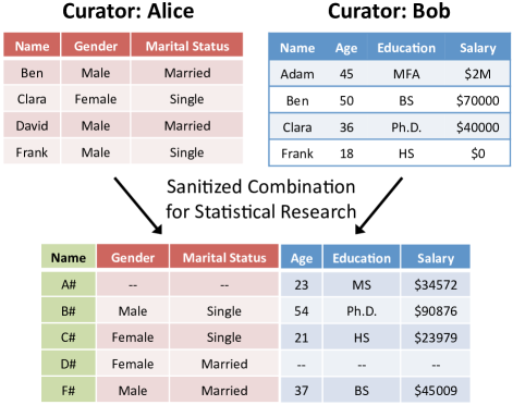
Figure 1: An example in which curators Alice and Bob hold vertically partitioned data, and a sanitized combination of their databases is made available for statistical analysis.

Recent research has shown that conventional mechanisms for privacy, such as $k$-anonymization [samarati01microdata, samaratiS98:protecting] do not provide adequate privacy. Specifically, an informed adversary can link an arbitrary amount of side information to the anonymized database, and defeat the anonymization mechanism [narayanan09ssp]. In response to vulnerabilities of simple anonymization mechanisms, a stricter notion of privacy — Differential Privacy [dwork08tamc, dwork09jpc] — has been developed in recent years. Informally, differential privacy ensures that the result of a function computed on a database of respondents is almost insensitive to the presence or absence of a particular respondent. A more formal way of stating this is that when the function is evaluated on adjacent databases (differing in only one respondent), the probability of outputting the same result is almost unchanged.

Mechanisms that provide differential privacy typically involve output perturbation, e.g., when Laplacian noise is added to the result of a function computed on a database, it provides differential privacy to the individual respondents in the database [smithlearn, diffrERM]. Nevertheless, it can be shown that input perturbation approaches such as the randomized response mechanism [warner65asa, warner71asa] – where noise is added to the data itself – also provide differential privacy to the respondents. In this work, we are interested in a privacy mechanism that achieves three goals. Firstly, the mechanism protects the privacy of individual respondents in a database. We achieve this through a privacy mechanism involving sampling and Post Randomization (PRAM) [gouweleeuwKWW98:PRAM], which is a generalization of randomized response. Secondly, the mechanism prevents unauthorized parties from learning anything about the data. We achieve this using random pads which can only be reversed by the authorized parties. Thirdly, the mechanism achieves a superior tradeoff between privacy and utility compared to simply performing PRAM on the database. We show that sampling the database enhances privacy with respect to the individual respondents while retaining the utility provided to an authorized researcher interested in the joint and marginal empirical probability distributions.

The idea of enhancing differential privacy via sampling, to the best of our knowledge, first appeared in [smithlearn, adamsamplingdp] and was further developed by [NinghuiSamplingDP]. Theorem III.2 that we develop and prove herein is analogous to the privacy amplification result of Theorem 1 in [NinghuiSamplingDP], however, the theorems are proved differently. Specifically, our proof requires an extra and non-trivial step because of the fact that the definition of differential privacy and sampling method in our setting are different. In the definition of differential privacy used in [smithlearn, adamsamplingdp, NinghuiSamplingDP], neighboring or adjacent databases are obtained by adding or deleting an entry from the database under consideration. This notion of adjacency cannot be used in our setting owing the fact that our setting involves perturbing the input data directly using techniques such as PRAM. In our work, an adjacent or neighboring database is obtained by replacing (i.e. deleting and adding) a single entry to the database under consideration. Further, the work in [smithlearn, adamsamplingdp, NinghuiSamplingDP] uses sampling with a fixed probability of including or excluding a sample, while our sampling mechanism is slightly different: the number of samples is fixed, and then sampling is carried out uniformly and without replacement based on the ratio of the number of samples to the size of the original database. This requires a different proof technique that considers sets of possible samplings.

The more significant difference with respect to recent work is that, unlike [NinghuiSamplingDP], we conduct a utility analysis, and derive a bound on the accuracy with which the desired statistical measures can be estimated, as a function of the noise inserted for privacy and the number of samples. Our analysis reveals a privacy-utility tradeoff between increasing PRAM noise versus decreasing the number of samples to maintain a desired level of differential privacy, and we determine the optimal number of samples that balances this tradeoff and maximizes the utility. We carry out experiments on both real-world and synthetically generated data which confirm the existence of this tradeoff, and reveal that the experimentally obtained optimal number of samples is very close to the number predicted by our analysis.

Another related work examines the effect of sampling on crowd-blending privacy [gehrkecrowd]. This is a strictly relaxed version of differential privacy, but it is shown that a pre-sampling step applied to a crowd-blending privacy mechanism can achieve a desired amount of differential privacy. The scenario in our work differs from the treatment in [gehrkecrowd] in that we consider vertically partitioned distributed databases which are held by mutually untrusting curators. In our setting, computing joint statistics requires a join operation on the databases, which implies that individual curators cannot independently blend their respondents without altering the joint statistics across all databases.

The remainder of this paper is organized as follows: Section II describes the multiparty problem setting, fixes notation and gives the privacy and utility definitions used in our analysis. Section III contains our main development, and begins by describing the mechanism itself, consisting of encryption via random padding, randomized sampling, and data perturbation. It is shown that sampling enhances the privacy of the individual respondents. An expression is derived for the utility function, namely the expected $\ell_{2}$-norm error in the estimate of the joint distribution, in terms of the number of samples and the amount of noise introduced by PRAM. More importantly, the analysis reveals a tradeoff between the number of samples and the perturbation noise. We conclude the section by deriving an expression for the optimal number of samples needed to maximize the utility function while achieving a desired level of privacy. In Section LABEL:sec:simulations, the claims made in the theoretical analysis are tested experimentally with the UCI “Adult Data Set” [Frank+Asuncion:2010] and with synthetically generated data. In particular, the theoretically predicted optimal number of samples, that minimizes the error in the joint distribution, is found to agree closely with the experimental results. Finally, Section LABEL:sec:discussion summarizes the main results and concludes the paper with a discussion on the practical considerations involved in performing privacy-preserving statistical analysis using a combination of encryption, sampling and data perturbation.

II Problem Formulation

Figure 2: Curators Alice and Bob independently encrypt their databases and provide it to a cloud server. The cloud server will sanitize the joint data. A researcher with decryption key can derive joint statistics or joint type based on the sanitized data, without compromising the privacy of individual database respondents. Neither the statistics nor the individual data entries are revealed to the cloud server.

In this section, we present our general problem setup, wherein database curators wish to release data to enable privacy-preserving data analysis by an authorized party. For ease of exposition, we present our problem formulation and results with two data curators, Alice and Bob, however our methods can easily be generalized to more than two curators. Consider a data mining application in which Alice and Bob are mutually untrusting data curators, as shown in Figure 2. The two databases are to be made available for research with authorization granted by the data curators, such that statistical measures can be computed either on the individual databases, or on some combination of the two databases. Data curators should have flexible access control over the data. For example, if a researcher is granted access by Alice but not by Bob, then he/she can only access Alice’s data. In addition, the cloud server should only host the data and not be able access the information. The data should be sanitized, before being released, to protect individual privacy. Altogether, we have the following privacy and utility requirements:

1. Database Security: Only researchers authorized by the data curators should be able to extract statistical information from the database.

2. Respondent Privacy: Individual privacy of the respondents must be maintained against the cloud server as well as the researchers.

3. Statistical Utility: An authorized researcher, i.e., one possessing appropriate keys, should be able to compute the joint and marginal distributions of the data provided by Alice and Bob.

4. Complexity: The overall communication and computation requirements of the system should be reasonable.

In the following sections, we will present our system framework and formalize the notions of privacy and utility.

II-A Type and Matrix Notation

The type (or empirical distribution) of a sequence $X^{n}$ is defined as the mapping $T_{X^{n}}:\mathcal{X}\rightarrow[0,1]$ given by

$$\forall x\in\mathcal{X},\quad T_{X^{n}}(x):=\frac{|\{i:X_{i}=x\}|}{n}.$$

The joint type of two sequences $X^{n}$ and $Y^{n}$ is defined as the mapping $T_{X^{n},Y^{n}}:\mathcal{X}\times\mathcal{Y}\rightarrow[0,1]$ given by

$$\forall(x,y)\in\mathcal{X}\times\mathcal{Y},\quad T_{X^{n},Y^{n}}(x,y):=\frac{|\{i:(X_{i},Y_{i})=(x,y)\}|}{n}.$$

For notational convenience, when working with finite-domain type/distribution functions, we will drop the arguments to represent and use these functions as vectors/matrices. For example, we can represent a distribution function $P_{X}:\mathcal{X}\rightarrow[0,1]$ as the $|\mathcal{X}|\times 1$ column-vector $P_{X}$, with its values arranged according to a fixed consistent ordering of $\mathcal{X}$. Thus, with a slight abuse of notation, using the values of $\mathcal{X}$ to index the vector, the “$x$”-th element of the vector, $P_{X}[x]$, is given by $P_{X}(x)$. Similarly, a conditional distribution function $P_{Y|X}:\mathcal{Y}\times\mathcal{X}\rightarrow[0,1]$ can be represented as a $|\mathcal{Y}|\times|\mathcal{X}|$ matrix $P_{Y|X}$, defined by $P_{Y|X}[y,x]:=P_{Y|X}(y|x)$. For example, by utilizing this notation, the elementary probability identity

$$\forall y\in\mathcal{Y},\quad P_{Y}(y)=\sum_{x\in\mathcal{X}}P_{Y|X}(y|x)P_{X}(x),$$

can be written in matrix form as simply $P_{Y}=P_{Y|X}P_{X}$.

II-B System Framework

Database Model: The data table held by Alice is modeled as a sequence $X^{n}:=(X_{1},X_{2},\ldots,X_{n})$, with each $X_{i}$ taking values in the finite-alphabet $\mathcal{X}$. Likewise, Bob’s data table is modeled as a sequence of random variables $Y^{n}:=(Y_{1},Y_{2},\ldots,Y_{n})$, with each $Y_{i}$ taking values in the finite-alphabet $\mathcal{Y}$. The length of the sequences, $n$, represents the total number of respondents in the database, and each $(X_{i},Y_{i})$ pair represents the data of the respondent $i$ collectively held by Alice and Bob, with the alphabet $\mathcal{X}\times\mathcal{Y}$ representing the domain of each respondent’s data.

Data Processing and Release: The curators each apply a data release mechanism to their respective data tables to produce an encryption of their data for the cloud server and a decryption key to be relayed to the researcher. These mechanisms are denoted by the randomized mappings $F_{A}:\mathcal{X}^{n}\rightarrow\mathcal{O}_{A}\times\mathcal{K}_{A}$ and $F_{B}:\mathcal{Y}^{n}\rightarrow\mathcal{O}_{B}\times\mathcal{K}_{B}$, where $\mathcal{K}_{A}$ and $\mathcal{K}_{B}$ are suitable key spaces, and $\mathcal{O}_{B}$ and $\mathcal{O}_{A}$ are suitable encryption spaces. The encryptions and keys are produced and given by

$$(O_{A},K_{A}):=F_{A}(X^{n}),$$

$$(O_{B},K_{B}):=F_{B}(Y^{n}).$$

The encryptions $O_{A}$ and $O_{B}$ are sent to the cloud server, which performs processing, and the keys $K_{A}$ and $K_{B}$ are later sent to the researcher. The cloud server processes $O_{A}$ and $O_{B}$, producing an output $O$ via a random mapping $M:\mathcal{O}_{A}\times\mathcal{O}_{B}\rightarrow\mathcal{O}$, as given by

$$O:=M(O_{A},O_{B}).$$

Statistical Recovery: To enable the recovery of the statistics of the database, the processed output $O$ is provided to the researcher via the cloud server, and the encryption keys $K_{A}$ and $K_{B}$ are provided by the curators. The researcher produces an estimate of the joint type (empirical distribution) of Alice and Bob’s sequences, denoted by $\widehat{T}_{X^{n},Y^{n}}$, as a function of $O$, $K_{A}$, and $K_{B}$, as given by

$$\widehat{T}_{X^{n},Y^{n}}:=g(O,K_{A},K_{B}),$$

where $g:\mathcal{O}\times\mathcal{K}_{A}\times\mathcal{K}_{B}\rightarrow[0,1]^{\mathcal{X}\times\mathcal{Y}}$ is the reconstruction function.

The objective is to design a system within the above framework, by specifying the mappings $F_{A}$, $F_{B}$, $M$, and $g$, that optimize the system performance requirements, which are formulated in the next subsection.

II-C Privacy and Utility Conditions

In this subsection, we formulate the privacy and utility requirements for our problem framework.

Privacy against the Server: In the course of system operation, the data curators do not want reveal any information about their data tables (not even aggregate statistics) to the cloud server. A strong statistical condition that guarantees this security is the requirement of statistical independence between the data tables and the encrypted versions held by the server. The statistical requirement of independence guarantees security even against an adversarial server with unbounded resources, and does not require any unproved assumptions.

Respondent Privacy: The data pertaining to a respondent should be kept private from all other parties, including any authorized researchers who aim to recover the statistics. We formalize this notion using $\epsilon$-differential privacy for the respondents as follows:

Definition II.1

[diffprivacy] Given the above framework, the system provides $\epsilon$-differential privacy if for all databases $(x^{n},y^{n})$ and $(\dot{x}^{n},\dot{y}^{n})$ in $\mathcal{X}^{n}\times\mathcal{Y}^{n}$, within Hamming distance $d_{H}((x^{n},y^{n}),(\dot{x}^{n},\dot{y}^{n}))\leq 1$, and all $\mathcal{S}\subseteq\mathcal{O}\times\mathcal{K}_{A}\times\mathcal{K}_{B}$,

$$\Pr\big{[}(O,K_{A},K_{B})\in\mathcal{S}\big{|}(X^{n},Y^{n})=(x^{n},y^{n})\big{]}$$

$$\quad\leq e^{\epsilon}\Pr\big{[}(O,K_{A},K_{B})\in\mathcal{S}\big{|}(X^{n},Y^{n})=(\dot{x}^{n},\dot{y}^{n})\big{]}$$

This rigorous definition of privacy is widely used and satisfies the privacy axioms of [privaxioms, privaxioms:journal]. Under the assumption that the respondents’ data is i.i.d., this definition results in a strong privacy guarantee: an attacker with knowledge of all except one of the respondents cannot recover the data of the sole missing respondent [Kifer11NoFreeLunch].

Utility for Authorized Researchers: The utility of the estimate is measured by the expected $\ell_{2}$-norm error of this estimated type vector, given by

$$E\big{\|}\widehat{T}_{X^{n},Y^{n}}-T_{X^{n},Y^{n}}\big{\|}_{2}$$

$$\quad:=\sqrt{\sum_{(x,y)\in\mathcal{X}\times\mathcal{Y}}\big{|}\widehat{T}_{X^{n},Y^{n}}(x,y)-T_{X^{n},Y^{n}}(x,y)\big{|}^{2}},$$

with the goal being the minimization of this error.

System Complexity: The communication and computational complexity of the system are also of concern. The computational complexity can be captured by the complexity of implementing the mappings ($F_{A}$, $F_{B}$, $M$ and $g$) that specify a given system. Ideally, one should aim to minimize the computational complexity of all of these mappings, simplifying the operations that each party must perform. The communication requirements is given by the cardinalities of the symbol alphabets ($\mathcal{O}_{A}$, $\mathcal{O}_{B}$, $\mathcal{K}_{A}$, $\mathcal{K}_{B}$, and $\mathcal{O}$). The logarithms of these alphabet sizes indicate the sufficient length for the messages that must be transmitted in this system.

III Proposed System and Analysis

In this section, we will present the details of our system, and analyze its privacy and utility performance. First, in Section III-A, we will describe how our system utilizes sampling and additive encryption, enabling a cloud server to join and perturb encrypted data in order to facilitate the release of sanitized data to the researcher. Next, in Section III-B, we analyze the privacy of our system and show that sampling enhances privacy, thereby reducing the amount of noise that must be injected during the perturbation step in order to obtain a desired level of privacy. Finally, in Section III-C, we analyze the accuracy of the joint type reconstruction, producing a bound on the utility as a function of the system parameters, viz., the noise added during perturbation, and the sampling factor.

III-A System Architecture

The data sanitization and release procedure is outlined by the following steps:

1. Sampling: The curators randomly sample their data, producing shortened sequences.

2. Encryption: The curators encrypt and send these shortened sequences to the cloud server.

3. Perturbation: The cloud server combines and perturbs the encrypted sequences.

4. Release: The researcher obtains the sanitized data from the server and the encryption keys from the curators, allowing the approximate recovery of data statistics.

A key aspect of these steps is that the encryption and perturbation schemes are designed such that these operations commute, thus allowing the server to essentially perform perturbation on the encrypted sequences, and for the authorized researcher to subsequently decrypt perturbed data. In this section, we describe the details of each step from a theoretical perspective by applying mathematical abstractions and assumptions. Later on, we will discuss practical implementations towards the realizing this system. The overall data sanitization process is illustrated in Figure 3.

Figure 3: Curators Alice and Bob independently encrypt their databases with a one time pad and provide it to a cloud server. The server samples $m$ respondents and then performs PRAM to guarantee privacy of the individual database respondents. A researcher can derive joint statistics or joint type based on the sanitized data, without compromising the privacy of the respondents. Neither the statistics nor the individual data entries are revealed to the cloud server.

Sampling: The data curators reduce their length-$n$ database sequences $(X^{n},Y^{n})$ to $m$ randomly drawn samples. We assume that these samples are drawn uniformly without replacement and that the curators will both sample at the same locations. We will let $(\widetilde{X}^{m},\widetilde{Y}^{m}):=(\widetilde{X}_{1},\ldots,\widetilde{X}_{m},\widetilde{Y}_{1},\ldots,\widetilde{Y}_{m})$ denote the intermediate result after sampling. Mathematically, the sampling result is described by, for all $i$ in $\{1,\ldots,m\}$,

$$(\widetilde{X}_{i},\widetilde{Y}_{i})=(X_{I_{i}},Y_{I_{i}}),$$

where $I_{1},\ldots,I_{m}$ are drawn uniformly without replacement from $\{1,\ldots,n\}$.

Encryption: The data curators independently encrypt their sampled data sequences with an additive (one-time pad) encryption scheme. To encrypt her data, Alice chooses an independent uniform key sequence $V^{m}\in\mathcal{X}^{m}$, and produces the encrypted sequence

$$\check{X}^{m}:=\widetilde{X}^{m}\oplus V^{m}:=(\widetilde{X}_{1}+V_{1},\ldots,\widetilde{X}_{m}+V_{m}),$$

where $\oplus$ denotes addition applied element-by-element over the sequences. Similarly, Bob encrypts his data, with the independent uniform key sequence $W^{m}\in\mathcal{Y}^{m}$, to produce the encrypted sequence

$$\check{Y}^{m}:=\widetilde{Y}^{m}\oplus W^{m}:=(\widetilde{Y}_{1}+W_{1},\ldots,\widetilde{Y}_{m}+W_{m}).$$

Alice and Bob send these encrypted sequences to the cloud server, and will provide the keys to the researcher to enable data release.

Perturbation: The cloud server joins the encrypted data sequences, forming $((\check{X}_{1},\check{Y}_{1}),\ldots,(\check{X}_{m},\check{Y}_{m}))$, and perturbs them by applying an independent PRAM mechanism, producing the perturbed results $(\overline{X}^{m},\overline{Y}^{m})$. Each joined and encrypted sample, $(\check{X}_{i},\check{Y}_{i})$, is perturbed independently and identically according to a conditional distribution, $P_{\overline{X},\overline{Y}|\check{X},\check{Y}}$, that specifies a random mapping from $(\mathcal{X}\times\mathcal{Y})$ to $(\mathcal{X}\times\mathcal{Y})$. Using the matrix $A:=P_{\overline{X},\overline{Y}|\check{X},\check{Y}}$ to represent the conditional distribution, this operation can be described by

$$P_{\overline{X}^{m},\overline{Y}^{m}|\check{X}^{m},\check{Y}^{m}}(\overline{x}^{m},\overline{x}^{m}|\check{x}^{m},\check{x}^{m})=\prod_{i=1}^{m}A[(\overline{x}_{i},\overline{y}_{i}),(\check{x}_{i},\check{y}_{i})].$$

By design, we specify that $A$ is a $\gamma$-diagonal matrix, for a parameter $\gamma>1$, given by

$$A[(\overline{x},\overline{y}),(\check{x},\check{y})]:=\begin{cases}\gamma/q,&\text{if}\ (\overline{x},\overline{y})=(\check{x},\check{y}),\\ 1/q,&\text{o.w.},\end{cases}$$

where $q:=(\gamma+|\mathcal{X}||\mathcal{Y}|-1)$ is a normalizing constant.

Release: In order to recover the data statistics, the researcher obtains the sampled, encrypted, and perturbed data sequences, $(\overline{X}^{m},\overline{Y}^{m})$, from the cloud server, and the encryption keys, $V^{m}$ and $W^{m}$, from the curators. The researcher decrypts and recovers the sanitized data given by

$$(\widehat{X}^{m},\widehat{Y}^{m}):=(\overline{X}^{m}\oplus V^{m},\overline{Y}^{m}\oplus W^{m}),$$

which is effectively the data sanitized by sampling and PRAM (see Lemma III.1 below). The researcher produces the joint type estimate by inverting the matrix $A$ and multiplying it with the joint type of the sanitized data as follows

$$\widehat{T}_{X^{n},Y^{n}}:=A^{-1}T_{\widehat{X}^{m},\widehat{Y}^{m}}.$$

Due to the $\gamma$-diagonal property of $A$, the PRAM perturbation is essentially an additive operation that commutes with the additive encryption. This allows the server to perturb the encrypted data, with the perturbation being preserved when the encryption is removed. The following Lemma summarizes this property, by stating that the decrypted, sanitized data recovered by the researcher, $(\widehat{X}^{m},\widehat{Y}^{m})$, is essentially the sampled data perturbed by PRAM.

Lemma III.1

Given the system described above, we have that

$$P_{\widehat{X}^{m},\widehat{Y}^{m}|\widetilde{X}^{m},\widetilde{Y}^{m}}(\widehat{x}^{m},\widehat{y}^{m}|\widetilde{x}^{m},\widetilde{y}^{m})=\prod_{i=1}^{m}A[(\widehat{x}_{i},\widehat{y}_{i}),(\widetilde{x}_{i},\widetilde{y}_{i})].$$

III-B Sampling Enhances Privacy

In this subsection, we will analyze the privacy of our proposed system. Specifically, we show how sampling in conjunction with PRAM enhances the overall privacy for the respondents in comparison to using PRAM alone. Note that if PRAM, with the $\gamma$-diagonal matrix $A$, was applied alone to the full databases, the resulting perturbed data would have $\ln(\gamma)$-differential privacy. In the following lemma, we will show that the combination of sampling and PRAM results in sampled and perturbed data with enhanced privacy.

Theorem III.2

The proposed system provides $\epsilon$-differential privacy for the respondents, where

$$\epsilon=\ln\left(\frac{n+m(\gamma-1)}{n}\right).$$ (1)

Proof:

The researcher receives the perturbed and encrypted data from the server $O:=(\overline{X}^{m},\overline{Y}^{m})$ and the keys $(K_{A},K_{B}):=(V^{m},W^{m})$ from the curators. However, since the sanitized data, $(\widehat{X}^{m},\widehat{Y}^{m})$, recovered by the researcher is a sufficient statistic for the original databases, that is, the following Markov chain holds

$$(X^{n},Y^{n})-(\widehat{X}^{m},\widehat{Y}^{m})-(\overline{X}^{m},\overline{Y}^{m},V^{m},W^{m}),$$

we need only to show that, for all $(x^{n},y^{n})$, $(\dot{x}^{n},\dot{y}^{n})$, and $(\widehat{x}^{m},\widehat{y}^{m})$ in $\mathcal{X}^{n}\times\mathcal{Y}^{n}$ with $d_{H}((x^{n},y^{n}),(\dot{x}^{n},\dot{y}^{n}))=1$,

$$\frac{P_{\widehat{X}^{m},\widehat{Y}^{m}|X^{n},Y^{n}}(\widehat{x}^{m},\widehat{y}^{m}|x^{n},y^{n})}{P_{\widehat{X}^{m},\widehat{Y}^{m}|X^{n},Y^{n}}(\widehat{x}^{m},\widehat{y}^{m}|\dot{x}^{n},\dot{y}^{n})}\leq e^{\epsilon},$$

in order to prove $\epsilon$-differential privacy for the respondents. Since $d_{H}((x^{n},y^{n}),(\dot{x}^{n},\dot{y}^{n}))=1$, the two database differ in only one location. Let $k$ denote the location where $(x_{k},y_{k})\neq(\dot{x}_{k},\dot{y}_{k})$.

Before we proceed, we introduce some notation regarding sampling to facilitate the steps of our proof. We will use the following notation for the set of all possible samplings

$$\Theta:=\big{\{}\pi|\pi:=(\pi_{1},\ldots,\pi_{m})\in\{1,\ldots,n\}^{m},\pi_{i}\neq\pi_{j},\forall i\neq j\big{\}}.$$

The sampling locations $(I_{1},\ldots,I_{m})$ are uniformly drawn from the set $\Theta$. We also define $\Theta_{k}:=\{\pi\in\Theta\,|\,\,\exists\,i,\pi_{i}=k\}$ to denote the subset of samplings that select location $k$, and $\Theta_{k}^{c}:=\Theta\setminus\Theta_{k}$ to denote the subset of samplings that do not select location $k$. For $\pi\in\Theta_{k}$, we define $\Theta_{k}(\pi):=\{\pi^{\prime}\in\Theta_{k}^{c}|d_{H}(\pi,\pi^{\prime})=1\}$ as the subset of $\Theta_{k}^{c}$ that replaces the selection of location $k$ with any other non-selected location. We will also slightly abuse notation by using $\pi\in\Theta$ as sampling function for the database sequences, that is, $\pi(X^{n}):=(X_{\pi_{1}},\ldots,X_{\pi_{m}})$, and similarly for $\pi(Y^{n})$. Using the above notation, we can rewrite the following conditional probability,

$$P_{\widehat{X}^{m},\widehat{Y}^{m}|X^{n},Y^{n}}(\widehat{x}^{m},\widehat{y}^{m}|x^{n},y^{n})$$

$$\ =\sum_{\pi\in\Theta}\frac{1}{|\Theta|}P_{\widehat{X}^{m},\widehat{Y}^{m}|\widetilde{X}^{m},\widetilde{Y}^{m}}\big{(}\widehat{x}^{m},\widehat{y}^{m}|\pi(x^{n}),\pi(y^{n})\big{)}$$

$$\ =\frac{1}{|\Theta|}\Big{[}\sum_{\pi\in\Theta_{k}}P_{\widehat{X}^{m},\widehat{Y}^{m}|\widetilde{X}^{m},\widetilde{Y}^{m}}\big{(}\widehat{x}^{m},\widehat{y}^{m}|\pi(x^{n}),\pi(y^{n})\big{)}$$

$$\quad+\sum_{\pi^{\prime}\in\Theta_{k}^{c}}P_{\widehat{X}^{m},\widehat{Y}^{m}|\widetilde{X}^{m},\widetilde{Y}^{m}}\big{(}\widehat{x}^{m},\widehat{y}^{m}|\pi^{\prime}(x^{n}),\pi^{\prime}(y^{n})\big{)}\Big{]}$$

$$\ =\frac{1}{|\Theta|}\Big{[}\sum_{\pi\in\Theta_{k}}\Big{(}P_{\widehat{X}^{m},\widehat{Y}^{m}|\widetilde{X}^{m},\widetilde{Y}^{m}}\big{(}\widehat{x}^{m},\widehat{y}^{m}|\pi(x^{n}),\pi(y^{n})\big{)}$$

$$\quad+\frac{1}{m}\sum_{\pi^{\prime}\in\Theta_{k}(\pi)}P_{\widehat{X}^{m},\widehat{Y}^{m}|\widetilde{X}^{m},\widetilde{Y}^{m}}\big{(}\widehat{x}^{m},\widehat{y}^{m}|\pi^{\prime}(x^{n}),\pi^{\prime}(y^{n})\big{)}\Big{)}\Big{]},$$

where in the last equality we have rearranged the summations to embed the summation over $\pi^{\prime}\in\Theta_{k}^{c}$ into the summation over $\pi\in\Theta_{k}$. Note that summing over all $\pi^{\prime}\in\Theta_{k}(\pi)$ within a summation over all $\pi\in\Theta_{k}$ covers all $\pi^{\prime}\in\Theta_{k}^{c}$, but overcounts each $\pi^{\prime}$ exactly $m$ times since each $\pi^{\prime}\in\Theta_{k}^{c}$ belongs to $m$ of the $\Theta_{k}(\pi)$ sets across all $\pi\in\Theta_{k}$. Hence, a $(1/m)$ term has been added to account for this overcount.

To ease the use of the above expansion, we introduce the following shorthand notation for the summation terms,

$$\alpha(\pi) :=P_{\widehat{X}^{m},\widehat{Y}^{m}|\widetilde{X}^{m},\widetilde{Y}^{m}}\big{(}\widehat{x}^{m},\widehat{y}^{m}|\pi(x^{n}),\pi(y^{n})\big{)}$$

$$\beta(\pi) :=P_{\widehat{X}^{m},\widehat{Y}^{m}|\widetilde{X}^{m},\widetilde{Y}^{m}}\big{(}\widehat{x}^{m},\widehat{y}^{m}|\pi(\dot{x}^{n}),\pi(\dot{y}^{n})\big{)}.$$

Thus, the following probability ratio can be written as

$$\frac{P_{\widehat{X}^{m},\widehat{Y}^{m}|X^{n},Y^{n}}(\widehat{x}^{m},\widehat{y}^{m}|x^{n},y^{n})}{P_{\widehat{X}^{m},\widehat{Y}^{m}|X^{n},Y^{n}}(\widehat{x}^{m},\widehat{y}^{m}|\dot{x}^{n},\dot{y}^{n})}$$

$$\quad=\frac{\sum_{\pi\in\Theta_{k}}\big{(}\alpha(\pi)+\frac{1}{m}\sum_{\pi^{\prime}\in\Theta_{k}(\pi)}\alpha(\pi^{\prime})\big{)}}{\sum_{\pi\in\Theta_{k}}\big{(}\beta(\pi)+\frac{1}{m}\sum_{\pi^{\prime}\in\Theta_{k}(\pi)}\beta(\pi^{\prime})\big{)}}$$

$$\quad\leq\max_{\pi\in\Theta_{k}}\frac{\alpha(\pi)+\frac{1}{m}\sum_{\pi^{\prime}\in\Theta_{k}(\pi)}\alpha(\pi^{\prime})}{\beta(\pi)+\frac{1}{m}\sum_{\pi^{\prime}\in\Theta_{k}(\pi)}\beta(\pi^{\prime})}$$

$$\quad=\frac{\alpha(\pi^{*})+\frac{1}{m}\sum_{\pi^{\prime}\in\Theta_{k}(\pi^{*})}\alpha(\pi^{\prime})}{\beta(\pi^{*})+\frac{1}{m}\sum_{\pi^{\prime}\in\Theta_{k}(\pi^{*})}\beta(\pi^{\prime})},$$

where $\pi^{*}\in\Theta_{k}$ denotes the sampling that maximizes the ratio. Given the $\gamma$-diagonal structure of the matrix $A$, we have that

$$\gamma^{-1}\alpha(\pi^{*})\leq\beta(\pi^{*}),$$

since $(\pi^{*}(x^{n}),\pi^{*}(y^{n}))$ and $(\pi^{*}(\dot{x}^{n}),\pi^{*}(\dot{y}^{n}))$ differ in only one location,

$$\gamma^{-1}\alpha(\pi^{*})\leq\alpha(\pi^{\prime}),\quad\forall\pi^{\prime}\in\Theta_{k}(\pi^{*}),$$

since $(\pi^{*}(x^{n}),\pi^{*}(y^{n}))$ and $(\pi^{\prime}(x^{n}),\pi^{\prime}(y^{n}))$ differ in only one location, and

$$\alpha(\pi^{\prime})=\beta(\pi^{\prime}),\quad\forall\pi^{\prime}\in\Theta_{k}(\pi^{*}),$$

since $(\pi^{\prime}(x^{n}),\pi^{\prime}(y^{n}))=(\pi^{\prime}(\dot{x}^{n}),\pi^{\prime}(\dot{y}^{n}))$. Given these constraints, we can continue to bound the likelihood ratio as

$$\frac{P_{\widehat{X}^{m},\widehat{Y}^{m}|X^{n},Y^{n}}(\widehat{x}^{m},\widehat{y}^{m}|x^{n},y^{n})}{P_{\widehat{X}^{m},\widehat{Y}^{m}|X^{n},Y^{n}}(\widehat{x}^{m},\widehat{y}^{m}|\dot{x}^{n},\dot{y}^{n})}$$

$$\quad\leq\frac{\alpha(\pi^{*})+\frac{1}{m}\sum_{\pi^{\prime}\in\Theta_{k}(\pi^{*})}\alpha(\pi^{\prime})}{\beta(\pi^{*})+\frac{1}{m}\sum_{\pi^{\prime}\in\Theta_{k}(\pi^{*})}\beta(\pi^{\prime})}$$

$$\quad\leq\frac{\alpha(\pi^{*})+\frac{n-m}{m}\gamma^{-1}\alpha(\pi^{*})}{\gamma^{-1}\alpha(\pi^{*})+\frac{n-m}{m}\gamma^{-1}\alpha(\pi^{*})}$$

$$\quad=\frac{n+m(\gamma-1)}{n}=e^{\epsilon},$$

thus finishing the proof by bounding the likelihood ratio with $e^{\epsilon}$. ∎

To show $\epsilon$-differential privacy for a given $\epsilon$, we only need to upperbound the probability ratio by $e^{\epsilon}$, as done in the above proof. A natural question is if this bound is tight, that is, whether there exists a smaller $\epsilon$ for which the bound also holds, hence making the system more private. With the following example, we show that the value for $\epsilon$ given in Theorem III.2 is tight.

Example III.3

Let $a$ and $b$ be two distinct elements in $(\mathcal{X}\times\mathcal{Y})$. Let $(x^{n},y^{n})=(b,a,a,\ldots,a)$, $(\dot{x}^{n},\dot{y}^{n})=(a,a,\ldots,a)$ and $(\widehat{x}^{m},\widehat{y}^{m})=(b,b,\ldots,b)$. Let $E$ denote the event that the first element (where the two databases differ) is sampled, which occurs with probability $(m/n)$. We can determine the likelihood ratio as follows

$$\frac{P_{\widehat{X}^{m},\widehat{Y}^{m}|X^{n},Y^{n}}(\widehat{x}^{m},\widehat{y}^{m}|x^{n},y^{n})}{P_{\widehat{X}^{m},\widehat{Y}^{m}|X^{n},Y^{n}}(\widehat{x}^{m},\widehat{y}^{m}|\dot{x}^{n},\dot{y}^{n})}$$

$$\quad=\frac{\Pr[E]\gamma(1/q)^{m}+(1-\Pr[E])(1/q)^{m}}{(1/q)^{m}}$$

$$\quad=\frac{n+m(\gamma-1)}{n}=e^{\epsilon}.$$

Thus, the value of $\epsilon$ given by Theorem III.2 is tight.

As a consequence of the privacy analysis of Theorem III.2, we have that for given system parameters of database length $n$, number of samples $m$, and desired level privacy $\epsilon$, the level of PRAM perturbation, specified by the $\gamma$ parameter of the matrix $A$, must be

$$\gamma=1+\frac{n}{m}(e^{\epsilon}-1).$$ (2)

Privacy against the server is obtained as a consequence of the one-time-pad encryption performed on the data prior to transmission to the server. It is straightforward to verify that the encryptions received by the server are statistically independent of the original database as a consequence of the independence and uniform randomness of the keys.

III-C Utility Analysis

In this subsection, we will analyze the utility of our proposed system. Our main result is a theoretical bound on the expected $\ell_{2}$-norm of the joint type estimation error. Analysis of this bound will illustrate the tradeoffs between utility and privacy level $\epsilon$ as function of sampling parameter $m$ and PRAM perturbation level $\gamma$. Given this error bound, we can compute the optimal sampling parameter $m$ for minimizing the error bound while achieving a fixed privacy level $\epsilon$.

Theorem III.4

For our proposed system, the expected $\ell_{2}$-norm of the joint type estimate is bounded by

$$E\big{\|}\widehat{T}_{X^{n},Y^{n}}-T_{X^{n},Y^{n}}\big{\|}_{2}\leq\frac{c\sqrt{|\mathcal{X}||\mathcal{Y}|}+1}{\sqrt{m}}.$$ (3)

where $c$ is the condition number of the $\gamma$-diagonal matrix $A$, given by

$$c=1+\frac{|\mathcal{X}||\mathcal{Y}|}{\gamma-1}.$$