Clustering for multivariate continuous and discrete longitudinal data

Abstract

Multiple outcomes, both continuous and discrete, are routinely gathered on subjects in longitudinal studies and during routine clinical follow-up in general. To motivate our work, we consider a longitudinal study on patients with primary biliary cirrhosis (PBC) with a continuous bilirubin level, a discrete platelet count and a dichotomous indication of blood vessel malformations as examples of such longitudinal outcomes. An apparent requirement is to use all the outcome values to classify the subjects into groups (e.g., groups of subjects with a similar prognosis in a clinical setting). In recent years, numerous approaches have been suggested for classification based on longitudinal (or otherwise correlated) outcomes, targeting not only traditional areas like biostatistics, but also rapidly evolving bioinformatics and many others. However, most available approaches consider only continuous outcomes as a basis for classification, or if noncontinuous outcomes are considered, then not in combination with other outcomes of a different nature. Here, we propose a statistical method for clustering (classification) of subjects into a prespecified number of groups with a priori unknown characteristics on the basis of repeated measurements of several longitudinal outcomes of a different nature. This method relies on a multivariate extension of the classical generalized linear mixed model where a mixture distribution is additionally assumed for random effects. We base the inference on a Bayesian specification of the model and simulation-based Markov chain Monte Carlo methodology. To apply the method in practice, we have prepared ready-to-use software for use in R (http://www.R-project.org). We also discuss evaluation of uncertainty in the classification and also discuss usage of a recently proposed methodology for model comparison—the selection of a number of clusters in our case—based on the penalized posterior deviance proposed by Plummer [Biostatistics 9 (2008) 523–539].

and T1Supported by the Czech Science Foundation Grant GAČR 201/09/P077. T2Supported by the Czech Science Foundation Grant GAČR P403/12/1557.

Arnost Komarek, Lenka Komarkova

1 Introduction

1.1 Data and the research question

In clinical practice multiple markers of disease progression, both continuous and discrete, are routinely gathered during the follow-up to decide on future treatment actions. Our work is motivated by data from a Mayo Clinic trial on 312 patients with primary biliary cirrhosis (PBC) conducted between 1974–1984 [Dickson et al. (1989)]. This longitudinal study had a median follow-up time of 6.3 years with a large number of clinical, biochemical, serological and histological parameters recorded for each patient. The data are available in Fleming and Harrington (1991), Appendix D, and electronically at http://lib.stat.cmu.edu/datasets/ pbcseq.

With these data, we shall mimic a common problem from the clinical practice: at a prespecified time point from the start of follow-up we want to use the values of the markers of the disease progression to identify groups of patients with similar characteristics. That is, we want to perform a cluster analysis using the longitudinal measurements. With these motivating data, we perform a classification of patients who survived without liver transplantation the first 910 days (2.5 years) of the study ($N=260$), the data being further referred to as PBC910. This corresponds to the practical problem outlined above, that is, clustering of patients being available at a given time point. For the purpose of this paper, the time point of 910 days was selected arbitrarily. Its choice in other application can, of course, be driven by practical or other considerations. The following markers will be considered for the cluster analysis: continuous logarithmic serum bilirubin (lbili), discrete platelet count (platelet) and dichotomous indication of blood vessel malformations (spiders); see Figure 1.

In a clinical routine usually only the last available measurements reflecting the current patient status are used to identify the prognostic groups—clusters. Clearly, such a procedure ignores the available information on the markers’ evolution over time, which might be more important for reasonable classification than simply the last known state. To remedy this deficiency, we shall propose a clustering method exploiting jointly the whole history of longitudinal measurements of all considered markers which might have a different nature from being continuous to discrete, or even dichotomous.

1.2 Basic notation and data characteristics

Let $\mathbf{Y}_{i,r}=(Y_{i,r,1},\ldots,\break Y_{i,r,n_{i,r}})^{\top}$ denote a random vector of the longitudinal profile of the $r$th marker ($r=1,\ldots,R$) pertaining to the $i$th subject ($i=1,\ldots,N$). Further, let $\mathbf{Y}_{i}=(\mathbf{Y}_{i,1}^{\top},\ldots,\mathbf{Y}_{i,R}^{\top})^{\top}$ be a random vector of all longitudinal measurements on the $i$th subject and $\mathbf{Y}=(\mathbf{Y}_{1}^{\top},\ldots,\mathbf{Y}_{N}^{\top})^{\top}$ a random vector representing all available outcomes. As usual, let $y_{i,r,j},\mathbf{y}_{i,r},\mathbf{y}_{i},\mathbf{y}$ denote the observed counterparts of corresponding upper case random variables and vectors. Throughout the paper, we will assume the independence of subjects, that is, independence of $\mathbf{Y}_{1},\ldots,\mathbf{Y}_{N}$. Furthermore, let $n=\sum_{i=1}^{N}\sum_{r=1}^{R}n_{i,r}$ be the total number of observations and let $t_{i,r,j}$ be the times (on a study time scale) at which the individual values $Y_{i,r,j}$ ($i=1,\ldots,N$, $r=1,\ldots,R$, $j=1,\ldots,n_{i,r}$) were taken. Finally, let $p(\cdot)$ and $p(\cdot|\cdot)$ be generic symbols for (conditional) distributions.

In the PBC910 data and our application, the number of markers $R$ equals 3. As it is common with the longitudinal data, numbers $n_{i,r}$ of available measurements of each marker varies (between 1 and 5) across patients (median 4), leading to $n=2734$. Further, the distribution of the time points $t_{i,r,j}$ also varies across subjects and markers; see Table 1. However, note that the fifth visit which is available for only three patients is not outlying with respect to its timing from the rest of the data set. Indeed, it only corresponds to patients with a slightly more frequent visiting schedule. In summary, our longitudinal data are heavily unbalanced and irregularly spaced in time, also containing 12 patients for whom only baseline marker values at time $t=0$ are available. It is our aim to also classify or at least suggest a classification for those patients.

Table 1: Data PBC910. Characteristics of the time points at which the longitudinal values of the markers for clustering were taken. For each marker $r$ and each visit $j$, $n_{r,j}^{*}$ gives the number of available measurements, med, $Q_{1}$ and $Q_{3}$ are the median, the lower and the upper quartile of the time points in months when the measurements were taken

	lbili $\bolds{(r=1)}$			platelet $\bolds{(r=2)}$			spiders $\bolds{(r=3)}$
		$\bolds{t_{i,r,j}}$ (months)			$\bolds{t_{i,r,j}}$ (months)			$\bolds{t_{i,r,j}}$ (months)
$\bolds{j}$	$\bolds{n_{r,j}^{*}}$	med	$\bolds{(Q_{1}$--$Q_{3})}$	$\bolds{n_{r,j}^{*}}$	med	$\bolds{(Q_{1}$--$Q_{3})}$	$\bolds{n_{r,j}^{*}}$	med	$\bolds{(Q_{1}$--$Q_{3})}$
1	260	00.0	(0.0–0.0)	256	00.0	(0.0–0.0)	260	00.0	(0.0–0.0)
2	248	06.1	(5.9–6.7)	241	06.1	(5.9–6.7)	247	06.1	(5.9–6.8)
3	226	12.2	(11.8–12.9)	224	12.2	(11.8–12.9)	224	12.2	(11.8–12.9)
4	181	24.3	(23.8–25.3)	180	24.3	(23.8–25.2)	180	24.3	(23.8–25.2)
5	003	23.4	(23.4–26.5)	002	23.4	(23.4–23.4)	002	23.4	(23.4–23.4)

1.3 Existing clustering methods, the need for extensions

In the literature numerous clustering methods applicable in many different situations are available. Nevertheless, as we discuss below, none of them is applicable for our problem of clustering where each subject is represented by a set of $R$, in general unbalanced and irregularly sampled longitudinal profiles of markers which may have a different nature starting from continuous and ending with a dichotomous one.

1.3.1 Classical approaches and a mixture model-based clustering

Apart from classical approaches like hierarchical clustering or $K$-means method [see, e.g., Hastie, Tibshirani and Friedman (2009), Chapter 13, Johnson and Wichern (2007), Chapter 12] and their many extensions, model-based clustering built on mixtures of parametric or even nonparametrically specified distributions assumed for random vectors $\mathbf{Y}_{1},\ldots,\mathbf{Y}_{N}$ has become quite popular in the past decade [e.g., Fraley and Raftery (2002)]. This is probably partially due to the availability of ready-to-use software like R [R Development Core Team (2012)] packages mclust of Fraley and Raftery (2006) for clustering based on mixtures of multivariate normal distributions, earlier versions of the mixAK package described by Komárek (2009) or mixtools of Benaglia et al. (2009), which also allows for nonparametric estimation of the mixture components. Another rapid evolution of model-based clustering algorithms also originates from their need in gene-expression data analysis [e.g., Newton and Chung (2010), Witten (2011)]. Nevertheless, classical approaches, model-based clustering based on mixtures of distributions and many other related methods are not applicable in our context.

Some of the above mentioned methods rely on distances based on a suitable metric between the observed values of underlying random vectors $\mathbf{Y}_{1},\ldots,\mathbf{Y}_{N}$ being viewed as points in the Euclidean space of a certain dimension. However, in our situation the dimension of each $\mathbf{Y}_{i}$ is generally different for each subject and typically random. Hence, it is even not possible to define a common sample space needed to define a reasonable metric to calculate the distances.

For model-based methods, on the other hand, it is necessary to assume that the random vectors $\mathbf{Y}_{1},\ldots,\mathbf{Y}_{N}$ are independent and, given the classification, identically distributed according to a suitable (multivariate) distribution. Neither of these can be assumed since for typical longitudinal data (including our PBC910 data) the measurements are taken at different time points for each subject and, hence, $\mathbf{Y}_{1},\ldots,\mathbf{Y}_{N}$ are hardly identically distributed even if the number of measurements was the same for all subjects (which is also not the case for our data).

1.3.2 Clustering based on a mixture of regression models

For data where the $i$th subject out of $N$ to be classified may be represented by one response random variable $Y_{i}$ and a vector of possibly fixed covariates $\mathbf{x}_{i}$, several methods for clustering based on mixtures of regression models have been developed. Among the first, Quandt and Ramsey (1978) assume a two-component mixture of two normal linear regressions. Extension into a general number of components and also a practically applicable implementation is provided by Benaglia et al. (2009). A variant of the clustering based on a mixture of regressions with application to gene-expression data is given by Qin and Self (2006). A generalization, allowing also for nonnormally distributed response random variables $Y_{1},\ldots,Y_{N}$, is due to Grün and Leisch (2007), who consider mixtures of generalized linear models. To apply these methods for our application, the single response random variables $Y_{i,r,j}$ could play the role of the response variables in the mixtures of regression models and the time points $t_{i,r,j}$ the role of the fixed covariates. Nevertheless, the clustering approaches based on mixtures of regression models are also ruled out in our situation since (a) we cannot assume a single parametric distribution for all response variables in the data since both continuous and discrete response variables appear in our data set, (b) each subject is in general represented by more than one pair (response, covariates).

1.3.3 Clustering approaches for functional data and stochastic processes

For given $r\in\{1,\ldots,R\}$, a set $\{\mathbf{Y}_{1,r},\ldots,\mathbf{Y}_{N,r}\}$ of longitudinal trajectories of the $r$th marker could also be viewed as a set of functional observations or, in more general, a set of realizations of a certain random process. A similar setting is also found in the applications in genomics where $\mathbf{Y}_{i,r}$ is typically a vector representing the expression curve of gene $i$ over time. In the functional data or genomics literature, several clustering methods have been developed for situations when it is possible to assume a decomposition of each observed value into

$$Y_{i,r,j}=m_{i,r}(t_{i,r,j})+\varepsilon_{i,r,j},\qquad i=1,\ldots,N,j=1,\ldots,n_{i},$$ (1)

where $m_{i,r}(t)$ is either the value of the underlying random functional or the mean $i$th gene-expression at time $t$ or, in general, the underlying stochastic process, and $\varepsilon_{i,r,j}$ $(i=1,\ldots,N,$ $j=1,\ldots,n_{i,r})$ are random variables with a zero mean and either a common variance $\sigma^{2}$ or subject/gene specific variances $\sigma_{i}^{2}$ $(i=1,\ldots,N)$. Based on this model (1), James and Sugar (2003) and Liu and Yang (2009) developed methods for the clustering of functional data. Peng and Müller (2008) proposed a distance-based clustering method and apply it to data from online auctions. For the genomics applications, Ramoni, Sebastiani and Kohane (2002) present an agglomerative clustering procedure based on the autoregressive model in equation (1). Another gene-expression clustering application based in fact on a mixture of regression models in equation (1) is provided by Ma et al. (2006). In our situation, these methods could only be applied if there is only one continuous marker available for each patient. Hence, with the PBC910 data, clustering would have to be based only on either lbili values or platelet values if it was assumed that they come from a continuous location-shift distribution. The dichotomous spiders values cannot be used at all.

1.3.4 Clustering based on mixture extensions of the mixed models

For the analysis of the continuous longitudinal data, the linear mixed model [LMM, Laird and Ware (1982)] plays a prominent role. For given $r\in\{1,\ldots,R\}$, it is based on expression

$$\mathbf{Y}_{i,r}=\mathbf{x}_{i,r}^{\top}\bolds{\alpha}_{r}+\mathbf{z}_{i,r}^{\top}\mathbf{b}_{i,r}+\bolds{\varepsilon}_{i,r},\qquad i=1,\ldots,N,$$ (2)

where $\mathbf{x}_{i,r}$ and $\mathbf{z}_{i,r}$ are vectors of fixed covariates containing the time points $t_{i,r,j}$ $(j=1,\ldots,n_{i,r})$ and possibly other factors. Further, $\bolds{\alpha}_{r}$ is a vector of unknown regression parameters, $\mathbf{b}_{i,r}$ are i.i.d. random variables—random effects with unknown mean $\bolds{\beta}_{r}$ and a covariance matrix $\mathbf{D}_{r}$, and $\bolds{\varepsilon}_{i,r}$ are independent random vectors with zero mean and a covariance matrix $\bolds{\Sigma}_{i,r}$. To cluster subjects based on the continuous longitudinal data, several approaches stemming from a mixture extension of the LMM (2) have been proposed in the literature. Verbeke and Lesaffre (1996) assume a normal mixture in the distribution of random effects and apply their method to clustering of growth curves, while Celeux, Martin and Lavergne (2005) consider a mixture of linear mixed models and perform clustering of gene-expression data. De la Cruz-Mesía, Quintana and Marshall (2008) proceed in a similar way, however, they replace the $\mathbf{x}_{i,r}^{\top}\bolds{\alpha}_{r}+\mathbf{z}_{i,r}^{\top}\mathbf{b}_{i,r}$ part of (2) by a nonlinear expression in $\bolds{\alpha}_{r}$ and $\mathbf{b}_{i,r}$.

By a suitable choice of the covariate vectors and imposing a suitable structure on the error covariance matrices $\bolds{\Sigma}_{i}$, it is possible to use the LMM (2) also for the analysis of $R>1$ continuous longitudinal markers and for clustering based on it as was done by Villarroel, Marshall and Barón (2009), or could be done using the model of Komárek et al. (2010) who performed the discriminant analysis, though. However, analogously to Section 1.3.3, all mentioned methods could be used for our application only if we wanted to base the clustering only on lbili and/or platelet values.

One possible strategy for clustering based on not only continuous longitudinal profiles is to use a general form of the model proposed by Booth, Casella and Hobert (2008) [equation (3) in their paper], where they assume that the (not necessarily normal) distribution of longitudinal observations of a particular marker depends on cluster-specific parameters and on a vector of random effects. Nevertheless, except for this general definition, they focus in their paper on a linear mixed model which is only applicable in situations when the observed longitudinal markers are continuous.

A specific option which allows for clustering based on a single longitudinal marker of a discrete nature is to replace the LMM (2) by a generalized linear mixed model [GLMM, e.g., Molenberghs and Verbeke (2005)] and assume a suitable mixture in the distribution of random effects [Spiessens, Verbeke and Komárek (2002)]. An example of clustering based on such a model is shown in Molenberghs and Verbeke (2005), Section 23.2. Nevertheless, it is still not possible to jointly use all three (in general, all $R$) markers.

1.3.5 Objectives and outline of the paper

In previous paragraphs we gave a brief overview of the most common classes of clustering approaches. We also argued that none of them are capable of exploiting jointly irregular longitudinal measurements of $R\geq 1$ markers of different nature (continuous, discrete or even dichotomous) as it is required by the PBC910 data. Even though our overview is by no means exhaustive, we are not aware of any method that would meet such needs. For these reasons we propose a clustering method that will be built upon the multivariate extension (where the word “multivariate” points to the fact that $R\geq 1$ markers will be modeled jointly) of the GLMM with a normal mixture in the distribution of random effects proposed by Spiessens, Verbeke and Komárek (2002), [SVK], and Molenberghs and Verbeke (2005), [MV]. Not only did they model just the $R=1$ longitudinal outcome, but they also considered only a homoscedastic normal mixture. Nevertheless, this is a rather restrictive assumption, especially in our context where each mixture component should represent one cluster. Hence, to have a better ground for clustering, the heteroscedastic mixture will be considered in our proposal. Further, in their illustrations, [SVK] and [MV] usually included at most bivariate random effects. This was probably due to the fact that as a method of estimation they exploited the maximum-likelihood through the EM algorithm which starts to be computationally troublesome for models with random effects of a higher dimension. For computational complexity implied by the multivariate extension of the mixture GLMM, but not only because of this, we shall use the Bayesian inference based on the Markov chain Monte Carlo (MCMC) simulation here.

In Section 2 we next describe the multivariate mixture generalized linear mixed model which will serve as the basis for our clustering procedure and show how to apply it to the PBC910 data. The clustering procedure will be described, and the clustering of patients from the PBC910 data will be performed in Section 3. In Section 4 we discuss the possibility of estimating a number of clusters needed in situations when this does not follow from the context. We evaluate the proposed methodology in Section 5 on a simulation study and finalize the paper by a discussion in Section 6.

2 Mixture multivariate generalized linear mixed model

2.1 Model specification

Our proposed clustering procedure is based on a multivariate mixture generalized linear mixed model (MMGLMM). We first express the conditional mean of each response profile using a standard GLMM, that is,

$$h_{r}^{-1}\bigl{\{}\mathsf{E}(Y_{i,r,j}|\bolds{\alpha}_{r},\mathbf{b}_{i,r})\bigr{\}}=\mathbf{x}_{i,r,j}^{\top}\bolds{\alpha}_{r}+\mathbf{z}_{i,r,j}^{\top}\mathbf{b}_{i,r},$$

(3)

$$\eqntext{i=1,\ldots,N,r=1,\ldots,R,j=1,\ldots,n_{i,r},}$$ (4)

where $h_{r}^{-1}$ is the link function used to model the mean of the $r$th marker, $\mathbf{x}_{i,r,j}$, $\mathbf{z}_{i,r,j}$ are vectors of known covariates which may include a constant for intercept, time values in which the longitudinal observations have been taken or any other additional covariates. Further, $\bolds{\alpha}_{r}$ is a vector of unknown regression coefficients (fixed effects) and $\mathbf{b}_{i,r}$ is a vector of random effects for the $r$th response specific for the $i$th subject. We assume hierarchically centered GLMM [Gelfand, Sahu and Carlin (1995)] where the random effects $\mathbf{b}_{1,r},\ldots,\mathbf{b}_{N,r}$ have in general a nonzero and unknown mean, let’s say $\bolds{\beta}_{r}$, $r=1,\ldots,R$; see equation (6) below. Being within the GLMM framework, we assume that for each $i=1,\ldots,N$, $r=1,\ldots,R$, $j=1,\ldots,n_{i,r}$, the conditional distribution $p(y_{i,r,j}|\phi_{r},\bolds{\alpha}_{r},\mathbf{b}_{i,r})$ belongs to an exponential family with the mean specified by (2.1), and possibly unknown dispersion parameter $\phi_{r}$. In a sequel, let $\bolds{\psi}=(\bolds{\phi}^{\top},\bolds{\alpha}^{\top})^{\top},$ where $\bolds{\alpha}=(\bolds{\alpha}_{1}^{\top},\ldots,\bolds{\alpha}_{R}^{\top})^{\top}$, $\bolds{\phi}=(\phi_{1}^{\top},\ldots,\phi_{R}^{\top})^{\top}$ is the vector of GLMM related parameters.

Further, let $\mathbf{b}_{i}=(\mathbf{b}_{i,1}^{\top},\ldots,\mathbf{b}_{i,R}^{\top})^{\top}$ be a joint vector of random effects for the $i$th subject $(i=1,\ldots,N)$. Dependence between the $R$ longitudinal markers of a particular subject $i$ represented by the response vectors $\mathbf{Y}_{i,1}$, $\ldots,$ $\mathbf{Y}_{i,R}$ is taken into account by assuming a joint distribution for the random effect vector $\mathbf{b}_{i}$ which also grounds our clustering procedure. We assume that the $i$th subject belongs to one of a fixed number of $K$ clusters (see Section 4 for possible approaches to choose $K$ if this does not follow from the context of the application at hand), each cluster with a probability $w_{k}=\mathsf{P}(u_{i}=k|\mathbf{w})$, $(0\leq w_{k}\leq 1$, $k=1,\ldots,K$, $\sum_{k=1}^{K}w_{k}=1)$, where $u_{i}\in\{1,\ldots,K\}$ is the $i$th subject allocation and $\mathbf{w}=(w_{1},\ldots,w_{K})^{\top}$. We further assume that the corresponding random effect vector $\mathbf{b}_{i}$ follows a multivariate normal distribution with an unknown mean $\bolds{\mu}_{u_{i}}$ and a (generally nondiagonal) unknown covariance matrix $\mathbf{D}_{u_{i}}$, that is,

$$p(\mathbf{b}_{i}|\bolds{\theta},u_{i}=k)=\varphi(\mathbf{b}_{i};\bolds{\mu}_{k},\mathbf{D}_{k}),\qquad i=1,\ldots,N,k=1,\ldots,K,$$

where $\varphi(\cdot|\bolds{\mu},\mathbf{D})$ is a density of the (multivariate) normal distribution with a mean $\bolds{\mu}$ and a covariance matrix $\mathbf{D}$, and $\bolds{\theta}=(\mathbf{w}^{\top},$ $\bolds{\mu}_{1}^{\top},\ldots,\bolds{\mu}_{K}^{\top},$ $\mathsf{\operatorname{vec}}(\mathbf{D}_{1}),\ldots,\break\mathsf{\operatorname{vec}}(\mathbf{D}_{K}))^{\top}$ is a vector of unknown parameters related to the distribution of random effects. That is, overall, we assume a multivariate normal mixture in the distribution of random effects:

$$\mathbf{b}_{i}|\bolds{\theta}\stackrel{{\scriptstyle\mathrm{i.i.d.}}}{{\sim}}\sum_{k=1}^{K}w_{k}\mathcal{MVN}(\bolds{\mu}_{k},\mathbf{D}_{k}),\qquad i=1,\ldots,N.$$ (5)

With this approach, we represent the unbalanced longitudinal observations $\mathbf{Y}_{1},\ldots,\mathbf{Y}_{N}$ using a set of i.i.d. random vectors $\mathbf{b}_{1},\ldots,\mathbf{b}_{N}$ which allows us to develop a clustering procedure based on ideas of the mixture model-based clustering introduced in Section 1.3.1.

Finally, we point out that given our model, the mean effect (in a total population) of covariates included in the vectors $\mathbf{z}_{i,r,j},$ $i=1,\ldots,N,$ $r=1,\ldots,R,$ $j=1,\ldots,n_{i,r}$ is given by

$$\bolds{\beta}=\sum_{k=1}^{K}w_{k}\bolds{\mu}_{k}.$$ (6)

This is a vector composed of $R$ subvectors, say, $\bolds{\beta}_{1},\ldots,\bolds{\beta}_{R}$, which play the role of the fixed effects for covariates included in the $z$-covariate vectors. Hence, for identifiability reasons, it is assumed that the vectors $\mathbf{x}_{i,r,j}$ and $\mathbf{z}_{i,r,j},$ $i=1,\ldots,N,$ $r=1,\ldots,R,$ $j=1,\ldots,n_{i,r}$ do not contain the same covariates.

2.2 Likelihood, Bayesian estimation

For largely computational reasons, we shall use the Bayesian inference based on the output from the MCMC simulation. To this end, the model must be specified also from a Bayesian point of view. A priori, we assume the independence between the mixture related parameters $\bolds{\theta}$ and the GLMM related parameters $\bolds{\psi}$. That is, the prior distribution $p(\bolds{\psi},\bolds{\theta})$ factorizes as $p(\bolds{\psi},\bolds{\theta})=p(\bolds{\psi})\times p(\bolds{\theta})$. The factorization of the prior is typical in generalized linear mixed models and might be justified in our application because the parameters involved in the $\bolds{\psi}$ and $\bolds{\theta}$ vector, respectively, express different features of the model. Specifically, for $p(\bolds{\theta})$, we use a multivariate version of the classical proposal of Richardson and Green (1997) as prior distribution, and, for $p(\bolds{\psi})$, we adopt classically used priors in this context [see, e.g., Fong, Rue and Wakefield (2010)]. A detailed description of the assumed form of $p(\bolds{\psi},\bolds{\theta})$ is provided in Appendix A of the Supplementary Material [Komárek and Komárková (2013)] where we also explain how to choose the prior hyperparameters in order to obtain a weakly informative prior distribution.

The likelihood of the MMGLMM follows from (2.1) and (5):

$$L(\bolds{\psi},\bolds{\theta})=p(\mathbf{y}|\bolds{\psi},\bolds{\theta})=\prod_{i=1}^{N}\Biggl{(}\sum_{k=1}^{K}w_{k}L_{i,k}(\bolds{\psi},\bolds{\theta})\Biggr{)},$$ (7)

where

$$L_{i,k}(\bolds{\psi},\bolds{\theta})=\int\Biggl{\{}\prod_{r=1}^{R}\prod_{j=1}^{n_{i,r}}p(y_{i,r,j}|\phi_{r},\bolds{\alpha}_{r},\mathbf{b}_{i,r})\Biggr{\}}p(\mathbf{b}_{i}|\bolds{\theta},u_{i}=k)\,d\mathbf{b}_{i},$$

(8)

$$\eqntext{i=1,\ldots,N,k=1,\ldots,K}$$ (9)

is the contribution of the $i$th subject to the likelihood under the assumption that the random effects are distributed according to the $k$th mixture component.

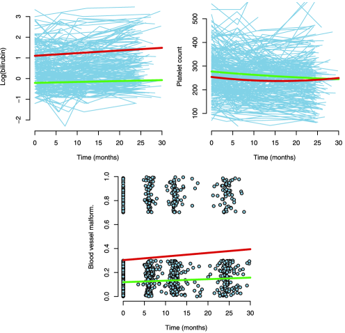
Figure 1: PBC910 data. Observed values of the longitudinal markers. Thick lines show cluster-specific marginal mean evolution over time based on posterior means of the mixture means $\bolds{\mu}_{1}$ (green) and $\bolds{\mu}_{2}$ (red). Observed values of dichotomous blood vessel malformations (spiders) are vertically jittered.

MCMC methods are used to generate a sample $\mathcal{S}_{M}=\{(\bolds{\psi}^{(m)},\bolds{\theta}^{(m)}):m=1,\ldots,M\}$ from the posterior distribution $p(\bolds{\psi},\bolds{\theta}|\mathbf{y})\propto L(\bolds{\psi},\bolds{\theta})\times p(\bolds{\psi},\bolds{\theta}).$ Namely, a block Gibbs algorithm is used with the Metropolis–Hastings steps for those blocks of model parameters where the normalizing constant of the full conditional distribution does not have a closed form. A well-known identifiability problem which arises from the invariance of the likelihood under permutation of the component labels is solved by applying the relabeling algorithm of Stephens (2000), which is suitable for mixture models targeted toward clustering in particular. For details of the MCMC algorithm, refer to Appendix B of the Supplement [Komárek and Komárková (2013)].

2.3 MMGLMM for the PBC910 data

The MMGLMM for the clustering of patients included in the PBC910 data will be based on longitudinal measurements of (1) logarithmic serum bilirubin (lbili, $Y_{i,1,j}$), (2) platelet counts (platelet, $Y_{i,2,j}$) and (3) dichotomous presence of blood vessel malformations (spiders, $Y_{i,3,j}$) with assumed (1) Gaussian, (2) Poisson and (3) Bernoulli distribution, respectively. Exploration of the observed longitudinal profiles (see also Figure 1) suggests the following form of the mean structure (2.1):

$$\mathsf{E}(Y_{i,1,j}|\mathbf{b}_{i,1}) = b_{i,1,1}+b_{i,1,2}t_{i,1,j},$$

$$\log\bigl{\{}\mathsf{E}(Y_{i,2,j}|\mathbf{b}_{i,2})\bigr{\}} = b_{i,2,1}+b_{i,2,2}t_{i,2,j},$$ (10)

$$\operatorname{logit}\bigl{\{}\mathsf{E}(Y_{i,3,j}|b_{i,3},\alpha_{3})\bigr{\}} = b_{i,3}+\alpha_{3}t_{i,3,j},$$

$i=1,\ldots,N$, $j=1,\ldots,n_{i,r}$, $r=1,2,3$, where $1\leq n_{i,r}\leq 5$. In model (2.3), $t_{i,r,j}$ is the time in months from the start of the follow-up when the value of $Y_{i,r,j}$ was obtained.

In the main analysis, we will classify patients into two groups and, hence, a two component mixture ($K=2$) will be considered in the distribution of five-dimensional random effect vector $\mathbf{b}_{i}=(b_{i,1,1},b_{i,1,2},$ $b_{i,2,1},b_{i,2,2},$ $b_{i,3})^{\top}$, where $b_{i,1,1},b_{i,2,1},b_{i,3}$ are random intercepts from the GLMM for each marker and $b_{i,1,2},b_{i,2,2}$ are random slopes from the GLMM for the first two markers. The model also involves the fixed effect $\bolds{\alpha}=\alpha_{3}$, the slope from the logit model for the third Bernoulli response and a dispersion parameter $\phi_{1}=\mathsf{\operatorname{var}}(Y_{i,1,j}|\mathbf{b}_{i,1})$, the residual variance from the Gaussian model for the first marker, the logarithmic bilirubin. Let $\sigma_{1}=\sqrt{\phi_{1}}$ be the corresponding residual standard deviation. The GLMM related parameters are thus $\bolds{\psi}=(\sigma_{1},\alpha_{3})^{\top}$. The results that we report are based on 10,000 iterations of 1:100 thinned MCMC obtained after a burn-in period of 1000 iterations. See Appendix C of the Supplement [Komárek and Komárková (2013)] for a full Bayesian specification of the model, particular choices of the hyperparameters, an illustration of the performance of the MCMC and detailed results.

With respect to clustering, the most important parameters are the mixture weights $w_{1}$, $w_{2}$ and the mixture means $\bolds{\mu}_{1}$, $\bolds{\mu}_{2}$ which characterize the clusters. Their estimates taken to be the posterior means (denoted by $\widehat{w}_{1},\widehat{w}_{2}$, $\widehat{\bolds{\mu}}_{1},\widehat{\bolds{\mu}}_{2}$, resp.) estimated from an appropriately relabeled MCMC sample are given in Table 2 together with the 95% highest posterior density credible intervals (HPD CI). The first cluster is thus characterized by a remarkably lower baseline bilirubin level and its slower increase over time compared to the second cluster. For the platelet counts, there is almost no difference between the clusters at the baseline and only a moderate difference with respect to the rate of its change, with the second cluster showing a faster decline. Finally, blood vessel malformations exhibit a higher probability in the second cluster compared to the first one. From the clinical point of view, the first cluster exhibits more favorable values and also an evolution of all three markers and, hence, it should correspond to patients with a better prognosis compared to the second cluster. We confirm this conclusion in Section 3.1 upon the classification of the individual patients.

Table 2: PBC910 data. Posterior means and 95% HPD credible intervals for mixture weights, mixture means and GLMM related parameters

	$\bolds{k=1}$	$\bolds{k=2}$
	$\bolds{\widehat{w}_{1}=\mathsf{E}(w_{1}|\mathbf{y})=0.598}$	$\bolds{\widehat{w}_{2}=\mathsf{E}(w_{2}|\mathbf{y})=0.402}$
Parameter	(0.471, 0.711)	(0.289, 0.529)
Logarithmic bilirubin (lbili)
Intercept	$-$0.209	1.102
$\widehat{\mu}_{k,1}=\mathsf{E}(\mu_{k,1}|\mathbf{y})$	($-$0.332, $-$0.082)	(0.828, 1.387)
Slope	0.00450	0.01281
$\widehat{\mu}_{k,2}=\mathsf{E}(\mu_{k,2}|\mathbf{y})$	(0.00056, 0.00818)	(0.00476, 0.02108)
Residual std. dev.	0.314
$\widehat{\sigma}_{1}=\mathsf{E}(\sigma_{1}|\mathbf{y})$	(0.294, 0.333)
Platelet count (platelet)
Intercept	5.58	5.46
$\widehat{\mu}_{k,3}=\mathsf{E}(\mu_{k,3}|\mathbf{y})$	(5.49, 5.65)	(5.35, 5.58)
Slope	$-$0.00567	$-$0.00828
$\widehat{\mu}_{k,4}=\mathsf{E}(\mu_{k,4}|\mathbf{y})$	($-$0.00799, $-$0.00339)	($-$0.01354, $-$0.00306)
Presence of blood vessel malformations (spiders)
Intercept	$-$4.33	$-$0.83
$\widehat{\mu}_{k,5}=\mathsf{E}(\mu_{k,5}|\mathbf{y})$	($-$5.90, $-$2.88)	($-$1.66, $-$0.02)
Slope	0.0280
$\widehat{\alpha}_{3}=\mathsf{E}(\alpha_{3}|\mathbf{y})$	(0.0026, 0.0532)

Table 3: PBC910 data. Standard deviations (on a diagonal) and correlations (off-diagonal elements) for each mixture component derived from the posterior means $\widehat{\mathbf{D}}_{1}=\mathsf{E}({\mathbf{D}}_{1}|\mathbf{y})$ and $\widehat{\mathbf{D}}_{2}=\mathsf{E}({\mathbf{D}}_{2}|\mathbf{y})$ of the mixture covariance matrices

	Intercept	Slope	Intercept	Slope	Intercept
	(lbili)	(lbili)	(platelet)	(platelet)	(spiders)
	$k=1$
Intercept (lbili)	0.428	$0.031$	$-0.282$	$-0.086$	$0.326$
Slope (lbili)		$0.00837$	$0.040$	$-0.214$	$0.100$
Intercept (platelet)			$0.309$	$-0.039$	$-0.042$
Slope (platelet)				$0.0105$	$0.028$
Intercept (spiders)					$4.02$
	$k=2$
Intercept (lbili)	0.776	$-0.183$	$0.119$	$-0.139$	$0.171$
Slope (lbili)		$0.03090$	$-0.034$	$0.249$	$0.116$
Intercept (platelet)			$0.398$	$-0.046$	$-0.191$
Slope (platelet)				$0.0232$	$-0.043$
Intercept (spiders)					$2.42$

To get a better idea of the meaning of the clusters, we used $\widehat{\bolds{\mu}}_{1}$ and $\widehat{\bolds{\mu}}_{2}$ together with the posterior means of the GLMM related parameters $\bolds{\psi}$ (see Table 2) and the posterior means of the mixture covariance matrices $\mathbf{D}_{1}$ and $\mathbf{D}_{2}$ (see Table 3), and calculated the estimates of the cluster specific (marginal) mean longitudinal evolutions $\mathsf{E}(Y_{\cdot,r,\cdot}|\bolds{\alpha}_{r},u=k)=\mathsf{E}_{\mathbf{b}}\{\mathsf{E}(Y_{\cdot,r,\cdot}|\mathbf{b},\bolds{\alpha}_{r},u=k)\}$, $k=1,2,$ $r=1,2,3$ over time. These are plotted as green ($k=1$) and red ($k=2$) lines on Figure 1.

3 Clustering procedure

It follows from the decision theory for classification [see Hastie, Tibshirani and Friedman (2009), Section 2.4] that the optimal classification of the $i$th subject ($i=1,\ldots,N$) is to be based on the posterior component probabilities $\pi_{i,k}=\mathsf{P}(u_{i}=k|\mathbf{y})$ $(k=1,\ldots,K)$. In our case, they are calculated by marginalization over the posterior distribution as

$$\pi_{i,k} = \int p_{i,k}(\bolds{\psi},\bolds{\theta})p(\bolds{\psi},\bolds{\theta}|\mathbf{y})\,d(\bolds{\psi},\bolds{\theta})=\mathsf{E}\bigl{\{}p_{i,k}(\bolds{\psi},\bolds{\theta})|\mathbf{y}\bigr{\}}$$

$$\approx \frac{1}{M}\sum_{m=1}^{M}p_{i,k}\bigl{(}\bolds{\psi}^{(m)},\bolds{\theta}^{(m)}\bigr{)}=\widehat{\pi}_{i,k},$$

where by Bayes’ rule

$$p_{i,k}(\bolds{\psi},\bolds{\theta})=\mathsf{P}(u_{i}=k|\bolds{\psi},\bolds{\theta},\mathbf{y}_{i})=\frac{w_{k}L_{i,k}(\bolds{\psi},\bolds{\theta})}{\sum_{l=1}^{K}w_{l}L_{i,l}(\bolds{\psi},\bolds{\theta})},$$

(12)

$$\eqntext{i=1,\ldots,N,k=1,\ldots,K.}$$ (13)

The $i$th subject is classically assigned to the cluster $g_{i}$ for which $\widehat{\pi}_{i,g_{i}}$ is largest among (3) [e.g., Titterington, Smith and Makov (1985), McLachlan and Basford (1988)].

In non-Bayesian applications, the clustering procedure is usually based on the values of $\widehat{p}_{i,k}=p_{i,k}(\widehat{\bolds{\psi}},\widehat{\bolds{\theta}})$, where $\widehat{\bolds{\psi}}$ and $\widehat{\bolds{\theta}}$ are suitable estimates (e.g., maximum-likelihood) of the model parameters. Only rarely the uncertainty in the estimation of $\widehat{p}_{i,k}$ expressed by evaluating their standard errors or calculating the confidence intervals is taken into account. This is probably because of the fact that $p_{i,k}(\bolds{\psi},\bolds{\theta})$ depend on the model parameters in a relatively complex way. In our case of the MMGLMM, it is, for example, complicated by the necessity to integrate the GLM likelihood over the assumed distribution of the random effects [see equation (2.2)], which in general does not have an analytic solution.

With the Bayesian approach followed in this paper, the values of $\widehat{\pi}_{i,k}$ used for clustering are the estimated posterior means of $p_{i,k}(\bolds{\psi},\bolds{\theta})$ and with the MCMC-based posterior inference, we can easily evaluate also the posterior standard deviations (counterparts of the classical standard errors) or the credible intervals (counterparts of the classical confidence intervals). These can be used to incorporate an uncertainty in the classification which, for example, in the clinical setting of the PBC910 data, can serve for the identification of subjects that should undergo additional screening before their ultimate classification; see Section 3.1.

3.1 Clustering of patients from the PBC910 data

Classification of patients according to the maximal value of the estimated posterior mean $\widehat{\pi}_{i,k}$ leads to 167 patients being classified in group 1 and 93 patients in group 2; see Figure 2. We argued in Section 2.3 that from a clinical point of view, the first group should correspond to patients with a better prognosis compared to the second group. With the PBC910 data, it is possible to confirm this conclusion since the information concerning the residual progression free survival time, defined as time till death due to liver complications or till liver transplantation, is available in the form of the classical right-censored data. We calculated Kaplan–Meier estimates of the survival probabilities based on data from patients classified in each group. These are plotted as solid lines on Figure 3. Indeed, the survival prognosis of group 1 is much better than that of group 2 with the estimated 5-year survival probability in group 1 of 0.934 compared to 0.554 in group 2, and the 10-year survival probabilities 0.679 and 0.141 in groups 1 and 2, respectively.

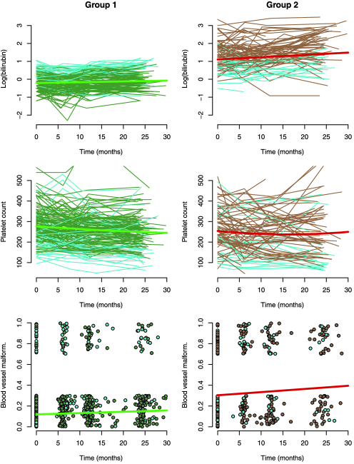
Figure 2: PBC910 data. Observed values of the longitudinal markers upon classification into $K=2$ groups. The thick lines show cluster-specific marginal mean evolution over time based on posterior means of the mixture means $\bolds{\mu}_{1}$ (green) and $\bolds{\mu}_{2}$ (red). Observed values of dichotomous blood vessel malformations (spiders) are vertically jittered. Profiles of patients for whom the lower limit of the 95% HPD credible interval did not exceed 0.5 are drawn in light blue.

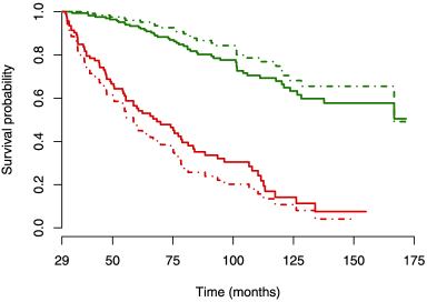
Figure 3: PBC910 data. Kaplan–Meier estimates of survival probability beyond 910 days in each group ($k=1$: green, $k=2$: red) created using the clustering procedure. Solid lines: everybody classified using the maximal value of $\widehat{\pi}_{i,k}$, dotted–dashed line: only patients for whom the lower limit of the 95% HPD CI for the component probability exceeded 0.5 were classified.

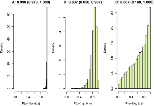
Figure 4: PBC910 data. Histograms of sampled values of component probabilities $p_{i,1}(\bolds{\psi},\bolds{\theta})$ for three selected patients. Above the plot: estimated posterior mean $\widehat{\pi}_{i,1}$ and the 95% HPD CI for $p_{i,1}=p_{i,1}(\bolds{\psi},\bolds{\theta})$.

The fact that the posterior means $\pi_{i,k}$ of the patient specific component probabilities characterize with different certainty the probabilities of the allocation for different patients is illustrated by Figure 4. It shows the MCMC-based estimates of the posterior distributions of the first component probabilities $p_{i,1}=p_{i,1}(\bolds{\psi},\bolds{\theta})$ for three selected patients who were all classified in a better prognosis group 1. For patient A, $\widehat{\pi}_{i,1}=0.990$ with a very narrow 95% HPD CI of $(0.970,1.000)$ and, thus, her classification in group 1 is almost certain. This is further confirmed by her progression-free survival time, which is almost 14 years. The posterior probability of belonging to group 1 is lower for patient C ($\widehat{\pi}_{i,1}=0.667$). Nevertheless, it is still twice as high as the posterior probability of belonging to group 2 ($\widehat{\pi}_{i,2}=0.333$) and, hence, it seems that patient C also belongs most likely in group 1. On the other hand, his progression-free survival time is only 3 years and 4 months (i.e., only 10 months beyond the time point at which we perform classification) and, hence, from a clinical point of view, this patient should rather be classified in group 2. In this case, the uncertainty in classification is expressed by a very wide 95% HPD CI which is $(0.168,1.000),$ covering the majority of the interval $(0,1)$.

In clinical practice, the diagnostic procedure usually proceeds in several steps, where in each step it is decided whether it is possible to classify a patient with enough certainty or whether additional examinations are needed before the ultimate classification is determined. Quite naturally, one of the diagnostic steps of such a procedure could be based on calculated credible intervals for individual component probabilities $p_{i,k}=p_{i,k}(\bolds{\psi},\bolds{\theta})$. The patient would be ultimately classified in one of the considered groups only if the lower limit of the corresponding credible interval exceeds a certain threshold, say, $0.5$ in the simplest case of classification into $K=2$ groups. Applying this procedure to the PBC910 data lead to 126 patients being classified in group 1 and 70 in group 2. In total, 64 patients (41 and 23 originally classified in group 1 and group 2, respectively, see light blue profiles on Figure 2) remain without ultimate classification, and additional screening or examinations would have been recommended for them before making a final decision. The fact that the two groups consisting of only 126 $+$ 70 ultimately classified patients better reflect the progression free survival status is illustrated by the Kaplan–Meier survival curves (dotted–dashed lines on Figure 3), which are now faster, diverting with the estimated 5-year survival probability in group 1 of 0.960 compared to 0.465 in group 2, and the 10-year survival probabilities 0.748 and 0.108 in groups 1 and 2, respectively.

4 Selection of a number of clusters

Until now, we assumed that the number of clusters, $K$, was known in advance and fixed. In medical applications where the found clusters are expected to correspond to certain prognostic groups, this is quite a reasonable assumption. Nevertheless, in many other situations, the number of clusters should rather be inferred from the data themselves.

With our approach, the selection of a number of clusters corresponds to the selection of a number of mixture components in the underlying distribution of the random effects of the MMGLMM. This can also be viewed as a problem of model selection or model comparison. Nevertheless, as described, for example, in McLachlan and Peel (2000), Chapter 6, the model comparison in the mixture setting is complicated by the fact that the classical regularity conditions do not hold. For this reason, use of various sorts of information criteria is predominantly preferred to classical testing in most frequentist applications of the mixture models. In particular, the Bayesian information criterion [BIC, Schwarz (1978)] proved to be a useful tool for selecting the number of mixture components [Dasgupta and Raftery (1998), Fraley and Raftery (2002), Hennig (2004), De la Cruz-Mesía, Quintana and Marshall (2008) and many others].

In Bayesian statistics, the Bayes factors [Kass and Raftery (1995)], for which the BIC is an approximation, are widely recognized as a tool of model selection. However, as pointed out by Plummer (2008), the Bayes factors have some practical limitations. First, they cannot be routinely calculated from the MCMC output. Second, they are numerically unstable when proper, but weakly informative diffused priors (as it is in our case) are used. In Bayesian applications, the deviance information criterion [DIC, Spiegelhalter et al. (2002)] seems to be the most widely used concept of model selection in the past decade. Nevertheless, DIC in the mixture context lacks the theoretical foundations and its use remains controversial [see comments and rejoinder on Celeux et al. (2006)]. For these reasons, Plummer (2008) suggested basing criteria for model choice on penalized loss functions and cross-validating arguments. For mixture models, in particular, he suggested using the penalized expected deviance (PED). Since then, it has been successfully exploited in several applications [Komárek (2009), Cabral, Lachos and Madruga (2012), De la Fé Rodríguez et al. (2011)], and we shall use it as well to choose the number of clusters.

The penalized expected deviance is defined as

$$\mathsf{\operatorname{PED}}=\mathsf{E}\bigl{\{}D(\bolds{\psi},\bolds{\theta})|\mathbf{y}\bigr{\}}+p_{\mathrm{opt}},$$ (14)

where $D(\bolds{\psi},\bolds{\theta})=-2\log\{L(\bolds{\psi},\bolds{\theta})\}$ is the observed data deviance of the model, and its posterior mean $\mathsf{E}\{D(\bolds{\psi},\bolds{\theta})|\mathbf{y}\}$ (expected deviance) is easily estimated from the MCMC sample. Further, the $p_{\mathrm{opt}}$ part of equation (14) is the penalty term called optimism, which can be estimated by using the two parallel MCMC chains and importance sampling [Plummer (2008)].

=200pt $\bolds{K}$ PED $\bolds{\widehat{\mathsf{E}}\{D(\bolds{\psi},\bolds{\theta})|\mathbf{y}\}}$ $\bolds{\widehat{p}}_{\mathbf{opt}}$ 1 14,277.9 14,241.8 0036.1 2 14,164.1 14,088.3 0075.8 3 14,183.1 14,057.1 0126.0 4 22,405.1 17,244.4 5160.8

Table 4: PBC910 data. Penalized expected deviance for models with $K=1,2,3,4$ clusters

4.1 Number of clusters in the PBC910 data

Table 4 shows calculated values of the penalized expected deviance for the PBC910 data and models with $K=1,2,3,4$ clusters. It shows that the two-component model fits the data clearly better than a model with just a single cluster. On the other hand, the three clusters are already too much for these data. Even though the expected deviance of the three-component model is lower than that of the two-component model, the decrease of the expected deviance is overcome by the penalization for the additional component.

The conclusion that the third cluster is redundant for our application is also supported by the fact that when a three-component model is fitted to the PBC910 data, the two components almost coincide with the mixture components from the $K=2$ model and the estimated weight of the additional component is only $\widehat{w}_{3}=0.021$, and only three patients are allocated here using the rule based on a maximal value of the posterior component probability.

5 A simulation study

5.1 Simulation setup

The setup of the simulation study was motivated by the PBC910 application and the data were generated according to the model (2.3). For each subject $i$ and each marker $r$, $n_{i,r}=4$ visit times were generated, with the first visit time being equal to 0 and the remaining three visit times being generated from uniform distributions on intervals $(170,200)$, $(350,390)$, $(710,770)$ days, respectively. The covariate $t_{i,r,j}$ in (2.3) was the visit time in months. The GLMM related parameters were equal: $\sigma_{1}=\sqrt{\phi_{1}}=0.3$, $\alpha_{3}=0.05$, and we tried two values for the true number of clusters: $K=2$ and $K=3$. In the two-cluster data, both mixture weights were rather high: $\mathbf{w}=(0.6,0.4)^{\top}$, whereas in the three-cluster data, a small third component with $w_{3}=0.06$ was created by splitting the second component of the two-cluster setting, leading to the weights $\mathbf{w}=(0.60,0.34,0.06)^{\top}$. To make the differences between the clusters less obvious, not all elements of the mixture means varied across the clusters; see Table 5. Namely, in data with $K=2$, both clusters shared the same value of the mean slope of the Gaussian response and also the same value of the mean intercept of the Poisson response. There were also some differences introduced across the mixture covariance matrices; see Table D.1 in the Supplement [Komárek and Komárková (2013)]. Example data sets generated according to considered simulation settings are also shown on Figures D.1 and D.2 of the Supplement.

== Proportion (%) of models selected with $K$ Setting $\bolds{\mathbf{w}}$ $\bolds{\mu_{*,1}}$ $\bolds{\mu_{*,2}}$ $\bolds{\mu_{*,3}}$ $\bolds{\mu_{*,4}}$ $\bolds{\mu_{*,5}}$ $\bolds{\alpha_{3}}$ Classif. error rate (%) 1 2 3 4 $K=2$ True values 0.600 0.000 $0.0100$ 5.00 $-0.0050$ $-3.00$ 0.050 0.400 1.000 $0.0100$ 5.00 $-0.0200$ $-1.00$ Square root of the MSE Normal $N=(30,20)$ 0.169 0.237 $0.0048$ 0.12 $0.0039$ $1.84$ 0.029 $15.8$ $67$ 33 00 0    $(60,40)$ 0.064 0.150 $0.0034$ 0.09 $0.0018$ $0.86$ 0.018 $7.8$ $15$ 85 00 0    $(120,80)$ 0.037 0.066 $0.0022$ 0.05 $0.0010$ $0.46$ 0.014 $5.8$ $1$ 99 00 0 MVT₅ $N=(30,20)$ 0.209 0.564 $0.0134$ 0.36 $0.0051$ $3.33$ 0.029 $20.6$ $64$ 35 01 0    $(60,40)$ 0.128 0.433 $0.0103$ 0.47 $0.0035$ $2.17$ 0.020 $10.8$ $17$ 76 07 0    $(120,80)$ 0.102 0.378 $0.0049$ 0.16 $0.0020$ $1.47$ 0.013 $8.7$ $0$ 82 18 0 $K=3$ True values 0.600 0.000 $0.0100$ 5.00 $-0.0050$ $-3.00$ 0.050 0.340 1.000 $0.0100$ 5.00 $-0.0200$ $-1.00$ 0.060 1.300 $-0.0300$ 5.50 $0.0000$ $-2.00$ Square root of the MSE Normal $N=(30,17,3)$ 0.154 0.444 $0.0204$ 0.33 $0.0073$ $5.04$ 0.027 $26.5$ $80$ 18 02 0    $(60,34,6)$ 0.088 0.360 $0.0165$ 0.26 $0.0054$ $3.07$ 0.018 $17.4$ $36$ 50 14 0    $(120,68,12)$ 0.048 0.260 $0.0126$ 0.19 $0.0034$ $1.58$ 0.015 $10.1$ $2$ 59 38 1 MVT₅ $N=(30,17,3)$ 0.113 0.563 $0.0237$ 0.52 $0.0078$ $3.99$ 0.021 $23.8$ $66$ 31 03 0    $(60,34,6)$ 0.122 0.424 $0.0211$ 0.31 $0.0058$ $2.66$ 0.021 $18.8$ $24$ 59 17 0    $(120,68,12)$ 0.056 0.353 $0.0196$ 0.22 $0.0048$ $1.56$ 0.013 $9.7$ $2$ 44 50 4

Table 5: Simulation study: (a) proportions of models selected with $K=1,2,3,4$ using the PED criterion; (b) total classification error rate from a model with correctly specified $K$; (c) true values of mixture weights and mixture means; (d) square roots of the mean squared errors (MSE), where the calculated MSE is based on posterior means as parameter estimates. For each parameter, the reported MSE is the average MSE over the $K$ mixture components. The $N$ gives the true number of subjects in each cluster

To examine the performance of our method in situations when there is misspecification in the random effects distribution, we simulated data not only under the normal distribution of random effects, but also under the shifted-scaled multivariate $t$-distribution with five degrees of freedom (MVT₅). For each setting ($K$, distribution of random effects), we tried three values of sample sizes with total numbers of subjects being $50,100,200$. For each setting and each sample size, 100 data sets were generated. The posterior inference for each data set was based on 10,000 iterations of 1:100 thinned MCMC obtained after a burn-in period of 1000 iterations.

5.2 Parameter estimates

The left block of Table 5 shows the square roots of the mean squared errors (MSE) in the estimation of the most important model parameters (mixture weights and means, GLMM fixed effects) provided that the number of clusters, $K$, is correctly specified. As parameter estimates, we considered the posterior means, and for a particular parameter the reported MSE is the average MSE over the parameter values from all $K$ components. Detailed results also providing the bias and the standard deviations of the posterior means are given in Tables D.3—D.6 of the Supplement [Komárek and Komárková (2013)].

With normally distributed random effects, the posterior means of model parameters seem to provide consistent estimates of the model parameters. The same can also be concluded when the true distribution of random effects is MVT₅. Nevertheless, not surprisingly, the convergence of the parameter estimates to their true values is in general slower in this case.

5.3 Classification error rates

With respect to classification, one of the most important measures is the classification error rate reported in the ninth column of Table 5. More detailed results, also showing conditional (given the cluster) classification error rates, are shown in Table D.2 of the Supplement [Komárek and Komárková (2013)]. Among other things, we point out that even with incorrectly specified distribution of random effects, the classification error rates do not differ considerably from the error rates obtained with data for which the random effects distribution was correctly specified, and even with a moderate sample size of 200 subjects, the achieved error rate is as low as 10%.

5.4 Selection of a number of clusters

Performance of the penalized expected deviance as a tool for the selection of a number of clusters is illustrated by the right block of Table 5. For each simulated data set, we estimated four models, each of them under the assumption of a different number of clusters, namely, $K=1,2,3,4$, and calculated the corresponding PED values. Table 5 shows proportions of data sets for which a particular number of clusters was selected by minimizing the PED. For each simulation setting, bold numbers indicate proportions of data sets with a correctly selected number of clusters.

For data sets composed of two clusters both having rather high weights, the probability of a selection of a correct model increases with the sample size, practically reaching 100% with $N=200$, and normally distributed random effects. The situation is slightly worse when the true distribution of random effects is MVT₅. Nevertheless, the results are also rather satisfactory in this case.

When there were three clusters present, with one of the clusters having a rather small weight of 0.06, the probability of a correct selection of a number of clusters also increases with the sample sizes (for both normally and MVT₅ distributed random effects). However, it is much slower than in the case of two clusters of almost equal size. Nevertheless, we point out that already for the moderate sample size of 200 subjects, in 97% and 94% of cases, respectively, the number of clusters indicated by the value of PED differs by at most one from the correct value of three.

6 Discussion

In this paper we have proposed a method for classification of subjects on the basis of longitudinal measurements of several outcomes of a different nature which, according to the best of our knowledge, has not been considered in the literature yet. The clustering procedure relies on a classical GLMM specified for each marker, whereas possible dependence across the values of different markers is captured by specifying a joint distribution of all random effects. In contrast to a classical assumption, we assume a normal mixture in the random effects distribution which is the core classification component of the proposed model. Although other choices of the basis distributions could be considered as well, we would like to stress the fact that with the Bayesian approach used here, the normality assumption only corresponds to a particular choice of just one component of the overall prior distribution which is updated by the data. For example, the posterior predictive distribution for random effects is given by

$$p_{\mathrm{pred}}(\mathbf{b})=\int\Biggl{\{}\sum_{k=1}^{K}w_{k}\varphi(\mathbf{b};\bolds{\mu}_{k},\mathbf{D}_{k})\Biggr{\}}p(\bolds{\theta}|\mathbf{y})\,d\bolds{\theta},$$

which in general is no longer a Gaussian mixture. In a similar way, the posterior distribution enters the calculation of the posterior component probabilities (3) while taking into account the uncertainty in the specification of the distribution of random effects. Last but not the least, the simulation study also suggests that, at least in situations when the true random effects distribution is symmetric with heavier tails, assuming a priori a normal random effects distribution does not have any crude impact on classification error rates.

Being within the Bayesian framework, it is also relatively easy to calculate not only point estimates of the individual component probabilities, but also corresponding credible intervals which can be subsequently used to evaluate uncertainty in the pertinence of a particular subject in a specific cluster. Such uncertainty is only rarely evaluated in similar situations. Finally, we adapted recently published methodology for model comparison based on the concept of a penalized expected deviance to explore the optimal number of clusters.

Further, we point out that even though we classified in this paper only those subjects who were also used to draw the posterior inference on the model parameters, our procedure can also be used to classify a new subject with a value of observed longitudinal markers equal to $\mathbf{y}_{\mathrm{new}}$ and unknown allocation $u_{\mathrm{new}}$. Indeed, given the posterior sample $\mathcal{S}_{M}$ from $p(\bolds{\psi},\bolds{\theta}|\mathbf{y})$, the component probabilities $p_{\mathrm{new},k}(\bolds{\psi}^{(m)},\bolds{\theta}^{(m)})$ and estimated posterior component probabilities $\widehat{\pi}_{\mathrm{new},k}$ $(k=1,\ldots,K)$ can be calculated using expressions (3) and (3), and then used for classification. Finally, it is worth mentioning that discriminant analysis, where a training data set with known cluster allocation is available, would also be possible with only slightly modified methodology where separate posterior samples would be drawn using the data from the various clusters and then used to calculate the component probabilities.

For practical analysis, we extended the R package mixAK [Komárek (2009)] to cover the methodology proposed in this paper. The package is freely available from the Comprehensive R Archive Network at http://cran.r-project.org/.

References

- Benaglia et al. (2009) {barticle}[author] \bauthor\bsnmBenaglia, \bfnmT.\binitsT., \bauthor\bsnmChauveau, \bfnmD.\binitsD., \bauthor\bsnmHunter, \bfnmD. R.\binitsD. R. and \bauthor\bsnmYoung, \bfnmD.\binitsD. (\byear2009). \btitleMixtools: An R package for analyzing finite mixture models. \bjournalJournal of Statistical Software \bvolume32 \bpages1–29. \bptokimsref \endbibitem
- Booth, Casella and Hobert (2008) {barticle}[mr] \bauthor\bsnmBooth, \bfnmJames G.\binitsJ. G., \bauthor\bsnmCasella, \bfnmGeorge\binitsG. and \bauthor\bsnmHobert, \bfnmJames P.\binitsJ. P. (\byear2008). \btitleClustering using objective functions and stochastic search. \bjournalJ. R. Stat. Soc. Ser. B Stat. Methodol. \bvolume70 \bpages119–139. \biddoi=10.1111/j.1467-9868.2007.00629.x, issn=1369-7412, mr=2412634 \bptokimsref \endbibitem
- Cabral, Lachos and Madruga (2012) {barticle}[mr] \bauthor\bsnmCabral, \bfnmCelso Rômulo Barbosa\binitsC. R. B., \bauthor\bsnmLachos, \bfnmVíctor Hugo\binitsV. H. and \bauthor\bsnmMadruga, \bfnmMaria Regina\binitsM. R. (\byear2012). \btitleBayesian analysis of skew-normal independent linear mixed models with heterogeneity in the random-effects population. \bjournalJ. Statist. Plann. Inference \bvolume142 \bpages181–200. \biddoi=10.1016/j.jspi.2011.07.007, issn=0378-3758, mr=2827140 \bptnotecheck year\bptokimsref \endbibitem
- Celeux, Martin and Lavergne (2005) {barticle}[mr] \bauthor\bsnmCeleux, \bfnmGilles\binitsG., \bauthor\bsnmMartin, \bfnmOlivier\binitsO. and \bauthor\bsnmLavergne, \bfnmChristian\binitsC. (\byear2005). \btitleMixture of linear mixed models for clustering gene expression profiles from repeated microarray experiments. \bjournalStat. Model. \bvolume5 \bpages243–267. \biddoi=10.1191/1471082X05st096oa, issn=1471-082X, mr=2210736 \bptokimsref \endbibitem
- Celeux et al. (2006) {barticle}[mr] \bauthor\bsnmCeleux, \bfnmG.\binitsG., \bauthor\bsnmForbes, \bfnmF.\binitsF., \bauthor\bsnmRobert, \bfnmC. P.\binitsC. P. and \bauthor\bsnmTitterington, \bfnmD. M.\binitsD. M. (\byear2006). \btitleDeviance information criteria for missing data models. \bjournalBayesian Anal. \bvolume1 \bpages651–673 (electronic). \bidissn=1931-6690, mr=2282197 \bptnotecheck related\bptokimsref \endbibitem
- Dasgupta and Raftery (1998) {barticle}[author] \bauthor\bsnmDasgupta, \bfnmA.\binitsA. and \bauthor\bsnmRaftery, \bfnmA. E.\binitsA. E. (\byear1998). \btitleDetecting features in spatial point processes with clutter via model-based clustering. \bjournalJ. Amer. Statist. Assoc. \bvolume93 \bpages294–302. \bptokimsref \endbibitem
- De la Cruz-Mesía, Quintana and Marshall (2008) {barticle}[mr] \bauthor\bparticleDe la \bsnmCruz-Mesía, \bfnmRolando\binitsR., \bauthor\bsnmQuintana, \bfnmFernando A.\binitsF. A. and \bauthor\bsnmMarshall, \bfnmGuillermo\binitsG. (\byear2008). \btitleModel-based clustering for longitudinal data. \bjournalComput. Statist. Data Anal. \bvolume52 \bpages1441–1457. \biddoi=10.1016/j.csda.2007.04.005, issn=0167-9473, mr=2422747 \bptokimsref \endbibitem
- De la Fé Rodríguez et al. (2011) {barticle}[author] \bauthor\bparticleDe la \bsnmFé Rodríguez, \bfnmP. Y.\binitsP. Y., \bauthor\bsnmCoddens, \bfnmA.\binitsA., \bauthor\bsnmDel Fava, \bfnmE.\binitsE., \bauthor\bsnmAbrahantes, \bfnmJ. C.\binitsJ. C., \bauthor\bsnmShkedy, \bfnmZ.\binitsZ., \bauthor\bsnmMartin, \bfnmL. O. M.\binitsL. O. M., \bauthor\bsnmMuñoz, \bfnmE. C.\binitsE. C., \bauthor\bsnmDuchateau, \bfnmL.\binitsL., \bauthor\bsnmCox, \bfnmE.\binitsE. and \bauthor\bsnmGoddeeris, \bfnmB. M.\binitsB. M. (\byear2011). \btitleHigh prevalence of F4+ and F18+Escherichia coli in Cuban piggeries as determined by serological survey. \bjournalTropical Animal Health and Production \bvolume43 \bpages937–946. \bptokimsref \endbibitem
- Dickson et al. (1989) {barticle}[pbm] \bauthor\bsnmDickson, \bfnmE. R.\binitsE. R., \bauthor\bsnmGrambsch, \bfnmP. M.\binitsP. M., \bauthor\bsnmFleming, \bfnmT. R.\binitsT. R., \bauthor\bsnmFisher, \bfnmL. D.\binitsL. D. and \bauthor\bsnmLangworthy, \bfnmA.\binitsA. (\byear1989). \btitlePrognosis in primary biliary cirrhosis: Model for decision making. \bjournalHepatology \bvolume10 \bpages1–7. \bidissn=0270-9139, pii=S0270913989001278, pmid=2737595 \bptokimsref \endbibitem
- Fleming and Harrington (1991) {bbook}[mr] \bauthor\bsnmFleming, \bfnmThomas R.\binitsT. R. and \bauthor\bsnmHarrington, \bfnmDavid P.\binitsD. P. (\byear1991). \btitleCounting Processes and Survival Analysis. \bpublisherWiley, \baddressNew York. \bidmr=1100924 \bptokimsref \endbibitem
- Fong, Rue and Wakefield (2010) {barticle}[pbm] \bauthor\bsnmFong, \bfnmYouyi\binitsY., \bauthor\bsnmRue, \bfnmHåvard\binitsH. and \bauthor\bsnmWakefield, \bfnmJon\binitsJ. (\byear2010). \btitleBayesian inference for generalized linear mixed models. \bjournalBiostatistics \bvolume11 \bpages397–412. \biddoi=10.1093/biostatistics/kxp053, issn=1468-4357, pii=kxp053, pmcid=2883299, pmid=19966070 \bptokimsref \endbibitem
- Fraley and Raftery (2002) {barticle}[mr] \bauthor\bsnmFraley, \bfnmChris\binitsC. and \bauthor\bsnmRaftery, \bfnmAdrian E.\binitsA. E. (\byear2002). \btitleModel-based clustering, discriminant analysis, and density estimation. \bjournalJ. Amer. Statist. Assoc. \bvolume97 \bpages611–631. \biddoi=10.1198/016214502760047131, issn=0162-1459, mr=1951635 \bptokimsref \endbibitem
- Fraley and Raftery (2006) {bmisc}[author] \bauthor\bsnmFraley, \bfnmC.\binitsC. and \bauthor\bsnmRaftery, \bfnmA. E.\binitsA. E. (\byear2006). \bhowpublishedMCLUST version 3 for R: Normal mixture modeling and model-based clustering. Technical Report 504, Dept. Statistics, Univ. Washington. \bptokimsref \endbibitem
- Gelfand, Sahu and Carlin (1995) {barticle}[mr] \bauthor\bsnmGelfand, \bfnmAlan E.\binitsA. E., \bauthor\bsnmSahu, \bfnmSujit K.\binitsS. K. and \bauthor\bsnmCarlin, \bfnmBradley P.\binitsB. P. (\byear1995). \btitleEfficient parameterisations for normal linear mixed models. \bjournalBiometrika \bvolume82 \bpages479–488. \biddoi=10.1093/biomet/82.3.479, issn=0006-3444, mr=1366275 \bptokimsref \endbibitem
- Grün and Leisch (2007) {barticle}[mr] \bauthor\bsnmGrün, \bfnmBettina\binitsB. and \bauthor\bsnmLeisch, \bfnmFriedrich\binitsF. (\byear2007). \btitleFitting finite mixtures of generalized linear regressions in . \bjournalComput. Statist. Data Anal. \bvolume51 \bpages5247–5252. \biddoi=10.1016/j.csda.2006.08.014, issn=0167-9473, mr=2370869 \bptokimsref \endbibitem
- Hastie, Tibshirani and Friedman (2009) {bbook}[mr] \bauthor\bsnmHastie, \bfnmTrevor\binitsT., \bauthor\bsnmTibshirani, \bfnmRobert\binitsR. and \bauthor\bsnmFriedman, \bfnmJerome\binitsJ. (\byear2009). \btitleThe Elements of Statistical Learning: Data Mining, Inference, and Prediction, \bedition2nd ed. \bpublisherSpringer, \baddressNew York. \biddoi=10.1007/978-0-387-84858-7, mr=2722294 \bptokimsref \endbibitem
- Hennig (2004) {barticle}[mr] \bauthor\bsnmHennig, \bfnmChristian\binitsC. (\byear2004). \btitleBreakdown points for maximum likelihood estimators of location-scale mixtures. \bjournalAnn. Statist. \bvolume32 \bpages1313–1340. \biddoi=10.1214/009053604000000571, issn=0090-5364, mr=2089126 \bptokimsref \endbibitem
- James and Sugar (2003) {barticle}[mr] \bauthor\bsnmJames, \bfnmGareth M.\binitsG. M. and \bauthor\bsnmSugar, \bfnmCatherine A.\binitsC. A. (\byear2003). \btitleClustering for sparsely sampled functional data. \bjournalJ. Amer. Statist. Assoc. \bvolume98 \bpages397–408. \biddoi=10.1198/016214503000189, issn=0162-1459, mr=1995716 \bptokimsref \endbibitem
- Johnson and Wichern (2007) {bbook}[mr] \bauthor\bsnmJohnson, \bfnmRichard A.\binitsR. A. and \bauthor\bsnmWichern, \bfnmDean W.\binitsD. W. (\byear2007). \btitleApplied Multivariate Statistical Analysis, \bedition6th ed. \bpublisherPearson Prentice Hall, \baddressUpper Saddle River, NJ. \bidmr=2372475 \bptokimsref \endbibitem
- Kass and Raftery (1995) {barticle}[author] \bauthor\bsnmKass, \bfnmR. E.\binitsR. E. and \bauthor\bsnmRaftery, \bfnmA. E.\binitsA. E. (\byear1995). \btitleBayes factors. \bjournalJ. Amer. Statist. Assoc. \bvolume90 \bpages773–795. \bptokimsref \endbibitem
- Komárek (2009) {barticle}[mr] \bauthor\bsnmKomárek, \bfnmArnošt\binitsA. (\byear2009). \btitleA new R package for Bayesian estimation of multivariate normal mixtures allowing for selection of the number of components and interval-censored data. \bjournalComput. Statist. Data Anal. \bvolume53 \bpages3932–3947. \biddoi=10.1016/j.csda.2009.05.006, issn=0167-9473, mr=2744295 \bptokimsref \endbibitem
- Komárek and Komárková (2013) {bmisc}[author] \bauthor\bsnmKomárek, \bfnmA.\binitsA. and \bauthor\bsnmKomárková, \bfnmL.\binitsL. (\byear2013). \bhowpublishedSupplement to “Clustering for multivariate continuous and discrete longitudinal data.” DOI:\doiurl10.1214/12-AOAS580SUPP. \bptokimsref \endbibitem
- Komárek et al. (2010) {barticle}[mr] \bauthor\bsnmKomárek, \bfnmArnošt\binitsA., \bauthor\bsnmHansen, \bfnmBettina E.\binitsB. E., \bauthor\bsnmKuiper, \bfnmEdith M. M.\binitsE. M. M., \bauthor\bparticlevan \bsnmBuuren, \bfnmHenk R.\binitsH. R. and \bauthor\bsnmLesaffre, \bfnmEmmanuel\binitsE. (\byear2010). \btitleDiscriminant analysis using a multivariate linear mixed model with a normal mixture in the random effects distribution. \bjournalStat. Med. \bvolume29 \bpages3267–3283. \biddoi=10.1002/sim.3849, issn=0277-6715, mr=2758719 \bptokimsref \endbibitem
- Laird and Ware (1982) {barticle}[pbm] \bauthor\bsnmLaird, \bfnmN. M.\binitsN. M. and \bauthor\bsnmWare, \bfnmJ. H.\binitsJ. H. (\byear1982). \btitleRandom-effects models for longitudinal data. \bjournalBiometrics \bvolume38 \bpages963–974. \bidissn=0006-341X, pmid=7168798 \bptokimsref \endbibitem
- Liu and Yang (2009) {barticle}[mr] \bauthor\bsnmLiu, \bfnmXueli\binitsX. and \bauthor\bsnmYang, \bfnmMark C. K.\binitsM. C. K. (\byear2009). \btitleSimultaneous curve registration and clustering for functional data. \bjournalComput. Statist. Data Anal. \bvolume53 \bpages1361–1376. \biddoi=10.1016/j.csda.2008.11.019, issn=0167-9473, mr=2657097 \bptokimsref \endbibitem
- Ma et al. (2006) {barticle}[pbm] \bauthor\bsnmMa, \bfnmPing\binitsP., \bauthor\bsnmCastillo-Davis, \bfnmCristian I.\binitsC. I., \bauthor\bsnmZhong, \bfnmWenxuan\binitsW. and \bauthor\bsnmLiu, \bfnmJun S.\binitsJ. S. (\byear2006). \btitleA data-driven clustering method for time course gene expression data. \bjournalNucleic Acids Res. \bvolume34 \bpages1261–1269. \biddoi=10.1093/nar/gkl013, issn=1362-4962, pii=34/4/1261, pmcid=1388097, pmid=16510852 \bptokimsref \endbibitem
- McLachlan and Basford (1988) {bbook}[mr] \bauthor\bsnmMcLachlan, \bfnmGeoffrey J.\binitsG. J. and \bauthor\bsnmBasford, \bfnmKaye E.\binitsK. E. (\byear1988). \btitleMixture Models: Inference and Applications to Clustering. \bseriesStatistics: Textbooks and Monographs \bvolume84. \bpublisherDekker, \baddressNew York. \bidmr=0926484 \bptokimsref \endbibitem
- McLachlan and Peel (2000) {bbook}[mr] \bauthor\bsnmMcLachlan, \bfnmGeoffrey\binitsG. and \bauthor\bsnmPeel, \bfnmDavid\binitsD. (\byear2000). \btitleFinite Mixture Models. \bpublisherWiley, \baddressNew York. \biddoi=10.1002/0471721182, mr=1789474 \bptokimsref \endbibitem
- Molenberghs and Verbeke (2005) {bbook}[mr] \bauthor\bsnmMolenberghs, \bfnmGeert\binitsG. and \bauthor\bsnmVerbeke, \bfnmGeert\binitsG. (\byear2005). \btitleModels for Discrete Longitudinal Data. \bpublisherSpringer, \baddressNew York. \bidmr=2171048 \bptokimsref \endbibitem
- Newton and Chung (2010) {barticle}[mr] \bauthor\bsnmNewton, \bfnmMichael A.\binitsM. A. and \bauthor\bsnmChung, \bfnmLisa M.\binitsL. M. (\byear2010). \btitleGamma-based clustering via ordered means with application to gene-expression analysis. \bjournalAnn. Statist. \bvolume38 \bpages3217–3244. \biddoi=10.1214/10-AOS805, issn=0090-5364, mr=2766851 \bptokimsref \endbibitem
- Peng and Müller (2008) {barticle}[mr] \bauthor\bsnmPeng, \bfnmJie\binitsJ. and \bauthor\bsnmMüller, \bfnmHans-Georg\binitsH.-G. (\byear2008). \btitleDistance-based clustering of sparsely observed stochastic processes, with applications to online auctions. \bjournalAnn. Appl. Stat. \bvolume2 \bpages1056–1077. \biddoi=10.1214/08-AOAS172, issn=1932-6157, mr=2516804 \bptokimsref \endbibitem
- Plummer (2008) {barticle}[pbm] \bauthor\bsnmPlummer, \bfnmMartyn\binitsM. (\byear2008). \btitlePenalized loss functions for Bayesian model comparison. \bjournalBiostatistics \bvolume9 \bpages523–539. \biddoi=10.1093/biostatistics/kxm049, issn=1468-4357, pii=kxm049, pmid=18209015 \bptokimsref \endbibitem
- Qin and Self (2006) {barticle}[mr] \bauthor\bsnmQin, \bfnmLi-Xuan\binitsL.-X. and \bauthor\bsnmSelf, \bfnmSteven G.\binitsS. G. (\byear2006). \btitleThe clustering of regression models method with applications in gene expression data. \bjournalBiometrics \bvolume62 \bpages526–533. \biddoi=10.1111/j.1541-0420.2005.00498.x, issn=0006-341X, mr=2236835 \bptokimsref \endbibitem
- Quandt and Ramsey (1978) {barticle}[mr] \bauthor\bsnmQuandt, \bfnmRichard E.\binitsR. E. and \bauthor\bsnmRamsey, \bfnmJames B.\binitsJ. B. (\byear1978). \btitleEstimating mixtures of normal distributions and switching regressions. \bjournalJ. Amer. Statist. Assoc. \bvolume73 \bpages730–738. \bidissn=0003-1291, mr=0521324 \bptnotecheck related\bptokimsref \endbibitem
- R Development Core Team (2012) {bmisc}[author] \borganizationR Development Core Team. (\byear2012). \bhowpublishedR: A Language and Environment for Statistical Computing. R Foundation for Statistical Computing, Vienna, Austria. ISBN 3-900051-07-0. Available at http://www.R-project.org. \bptokimsref \endbibitem
- Ramoni, Sebastiani and Kohane (2002) {barticle}[mr] \bauthor\bsnmRamoni, \bfnmMarco F.\binitsM. F., \bauthor\bsnmSebastiani, \bfnmPaola\binitsP. and \bauthor\bsnmKohane, \bfnmIsaac S.\binitsI. S. (\byear2002). \btitleCluster analysis of gene expression dynamics. \bjournalProc. Natl. Acad. Sci. USA \bvolume99 \bpages9121–9126 (electronic). \biddoi=10.1073/pnas.132656399, issn=1091-6490, mr=1909705 \bptokimsref \endbibitem
- Richardson and Green (1997) {barticle}[mr] \bauthor\bsnmRichardson, \bfnmSylvia\binitsS. and \bauthor\bsnmGreen, \bfnmPeter J.\binitsP. J. (\byear1997). \btitleOn Bayesian analysis of mixtures with an unknown number of components. \bjournalJ. Roy. Statist. Soc. Ser. B \bvolume59 \bpages731–792. \biddoi=10.1111/1467-9868.00095, issn=0035-9246, mr=1483213 \bptnotecheck related\bptokimsref \endbibitem
- Schwarz (1978) {barticle}[mr] \bauthor\bsnmSchwarz, \bfnmGideon\binitsG. (\byear1978). \btitleEstimating the dimension of a model. \bjournalAnn. Statist. \bvolume6 \bpages461–464. \bidissn=0090-5364, mr=0468014 \bptokimsref \endbibitem
- Spiegelhalter et al. (2002) {barticle}[mr] \bauthor\bsnmSpiegelhalter, \bfnmDavid J.\binitsD. J., \bauthor\bsnmBest, \bfnmNicola G.\binitsN. G., \bauthor\bsnmCarlin, \bfnmBradley P.\binitsB. P. and \bauthor\bparticlevan der \bsnmLinde, \bfnmAngelika\binitsA. (\byear2002). \btitleBayesian measures of model complexity and fit. \bjournalJ. R. Stat. Soc. Ser. B Stat. Methodol. \bvolume64 \bpages583–639. \biddoi=10.1111/1467-9868.00353, issn=1369-7412, mr=1979380 \bptnotecheck related\bptokimsref \endbibitem
- Spiessens, Verbeke and Komárek (2002) {bmisc}[author] \bauthor\bsnmSpiessens, \bfnmB.\binitsB., \bauthor\bsnmVerbeke, \bfnmG.\binitsG. and \bauthor\bsnmKomárek, \bfnmA.\binitsA. (\byear2002). \bhowpublishedA SAS-macro for the classification of longitudinal profiles using mixtures of normal distributions in nonlinear and generalised linear mixed models. Technical Report, Biostatistical Center, Catholic Univ. Leuven, Leuven. \bptokimsref \endbibitem
- Stephens (2000) {barticle}[mr] \bauthor\bsnmStephens, \bfnmMatthew\binitsM. (\byear2000). \btitleDealing with label switching in mixture models. \bjournalJ. R. Stat. Soc. Ser. B Stat. Methodol. \bvolume62 \bpages795–809. \biddoi=10.1111/1467-9868.00265, issn=1369-7412, mr=1796293 \bptokimsref \endbibitem
- Titterington, Smith and Makov (1985) {bbook}[mr] \bauthor\bsnmTitterington, \bfnmD. M.\binitsD. M., \bauthor\bsnmSmith, \bfnmA. F. M.\binitsA. F. M. and \bauthor\bsnmMakov, \bfnmU. E.\binitsU. E. (\byear1985). \btitleStatistical Analysis of Finite Mixture Distributions. \bpublisherWiley, \baddressChichester. \bidmr=0838090 \bptokimsref \endbibitem
- Verbeke and Lesaffre (1996) {barticle}[author] \bauthor\bsnmVerbeke, \bfnmG.\binitsG. and \bauthor\bsnmLesaffre, \bfnmE.\binitsE. (\byear1996). \btitleA linear mixed-effects model with heterogeneity in the random-effects population. \bjournalJ. Amer. Statist. Assoc. \bvolume91 \bpages217–221. \bptokimsref \endbibitem
- Villarroel, Marshall and Barón (2009) {barticle}[mr] \bauthor\bsnmVillarroel, \bfnmLuis\binitsL., \bauthor\bsnmMarshall, \bfnmGuillermo\binitsG. and \bauthor\bsnmBarón, \bfnmAnna E.\binitsA. E. (\byear2009). \btitleCluster analysis using multivariate mixed effects models. \bjournalStat. Med. \bvolume28 \bpages2552–2565. \biddoi=10.1002/sim.3632, issn=0277-6715, mr=2750308 \bptokimsref \endbibitem
- Witten (2011) {barticle}[mr] \bauthor\bsnmWitten, \bfnmDaniela M.\binitsD. M. (\byear2011). \btitleClassification and clustering of sequencing data using a Poisson model. \bjournalAnn. Appl. Stat. \bvolume5 \bpages2493–2518. \biddoi=10.1214/11-AOAS493, issn=1932-6157, mr=2907124 \bptokimsref \endbibitem