Sinc-based method for an efficient solution in the direct space of quantum wave equations with periodic boundary conditions

Abstract

The solution of differential problems, and in particular of quantum wave equations, can in general be performed both in the direct and in the reciprocal space. However, to achieve the same accuracy, direct-space finite-difference approaches usually involve handling larger algebraic problems with respect to the approaches based on the Fourier transform in reciprocal space. This is the result of the errors that direct-space discretization formulas introduce into the treatment of derivatives. Here, we propose an approach, relying on a set of sinc-based functions, that allows us to achieve an exact representation of the derivatives in the direct space and that is equivalent to the solution in the reciprocal space. We apply this method to the numerical solution of the Dirac equation in an armchair graphene nanoribbon with a potential varying only in the transverse direction.

I Introduction

With the progressive downscaling of electron devices, whose size has reached well into the nanoscale, the quantum simulation of charge transport has become increasingly important. This study requires the numerical solution of the quantum wave equation for the charge carriers in the device.

In the case of periodic boundary conditions, the solution in the Fourier domain represents a spontaneous alternative to a study in the direct space. In a Fourier analysis, all the functions appearing in the equation are replaced by their Fourier expansions, and the Fourier coefficients of the wave function become the unknowns of the problem, which in direct space approaches are instead the values of the wave function at the points of a discretization grid.

The main advantage of this technique is the correct treatment of the derivatives. In a reciprocal space analysis, each of the complex exponential functions appearing in the Fourier expansions can be derived exactly, without any approximation. On the contrary, in a standard finite difference solution, the derivatives are replaced with finite difference approximations involving a certain number of samples of the function. This approximation introduces a distortion in the dispersion relation, which severely limits the accuracy of high-order solutions. The discretization error decreases if a finer grid is used, at the expense of an increase of the computational effort. Moreover, in some cases, such as the solution of the Dirac equation for massless fermions, the discretization of the equation on a direct space grid gives rise to problems such as the appearance of spurious solutions, or fermion doubling, unless proper, non-standard discretization techniques are applied, stacey1982 ; bender1983 ; susskind1977 while these issues do not appear using a Fourier solution technique. The solution in the reciprocal space is especially convenient when a continuum, envelope function description of the device is adopted and a slowly varying potential (containing only a limited number of Fourier components) is considered.

Here, we illustrate how the use of a particular set of periodic basis functions, obtained from the periodic repetition of sinc (cardinal sine) functions, makes it possible to obtain an exact description of the derivatives in the direct space and a solution approach equivalent to that in the reciprocal space. This approach allows solving the differential problem in a very efficient way in the direct space, without the need to switch to the reciprocal space and vice versa.

After a general presentation (in Sec. II) of the method that we propose, in Secs. III and IV we describe how each term of the differential equation is treated, and in Sec. V, we demonstrate the equivalence of the sinc-based method to a Fourier approach.

Finally, in Sec. VI, we apply this method to the solution of the the wave equation in an armchair graphene nanoribbon (described using an envelope function approach) with a potential varying only in the transverse direction. Graphene represents an interesting material that, since its isolation in 2004 geim , has been the focus of a vast theoretical and experimental research activity rise ; status ; castroneto ; experimental ; mikhailov ; connolly ; iwceconn ; acsnano ; iwceroche . Among the many applications that have been proposed for this material, the possibility to use graphene nanoribbons for the implementation of nanoelectronic devices raza ; schwierz ; persp is particularly intriguing. The effective wave equation for the envelope functions, which in common semiconductors corresponds to the effective mass Schrödinger equation yu ; mitin (see, for example, Refs. epl ; prl ; prb ; fnl ; cavita ), in monolayer graphene is represented by the Dirac equation ando ; kp . Its numerical solution in graphene ribbons with an arbitrary potential landscape has been studied in a few recent papers tworzydlo2008 ; hernandez2012 ; snyman2008 . The solution of the Dirac equation within a slice with a potential varying only in the transverse direction can be exploited to perform a transport analysis for an armchair nanoribbon with a generic potential, if we subdivide the ribbon into a series of slices in each of which the potential is approximately constant in the longitudinal direction, and then we apply a recursive technique to obtain the transmission through the overall device icnf2013 .

II Mathematical method

For the sampling theorem, if a function $z(x)$ is band limited with band $B\leq 1/(2\,\Delta)$ (Nyquist criterion), it can be perfectly reconstructed haykin from its samples taken with a sampling interval $\Delta$

$$z(x)=\sum_{n=-\infty}^{+\infty}z(n\,\Delta)\,{\rm sinc}\left(\frac{x-n\Delta}{\Delta}\right)\,,$$ (1)

where the sinc function is defined as ${\rm sinc}(x)\equiv\sin(\pi x)/(\pi x)$.

Moreover, if $z(x)$ is periodic with period $L$ and we take $N$ samples within a period (and thus $L=N\,\Delta$), we have that

$$z(x) = \sum_{\ell=0}^{N-1}\sum_{\eta=-\infty}^{+\infty}z((\ell+\eta N)\Delta)\,\,{\rm sinc}\left(\frac{x-(\ell+\eta N)\Delta}{\Delta}\right)$$ (2)

$$= \sum_{\ell=0}^{N-1}z(\ell\,\Delta)\sum_{\eta=-\infty}^{+\infty}{\rm sinc}\left(\frac{x-(\ell+\eta N)\Delta}{\Delta}\right)$$

$$= \sum_{\ell=0}^{N-1}z(\ell\,\Delta)g_{\ell,\Delta}(x)\,,$$

where we have exploited the periodicity of $z(x)$ and we have defined the function (periodic with period $L=N\,\Delta$)

$$g_{\ell,\Delta}(x)\equiv\sum_{\eta=-\infty}^{+\infty}{\rm sinc}\left(\frac{x-(\ell+\eta N)\Delta}{\Delta}\right)$$ (3)

(in Fig. 1, we represent 4 periods of the function $g_{\ell,\Delta}(x)$ for $N=15$ and $\ell=5$).

Figure 1: Four periods of the function $g_{\ell,\Delta}(x)$ for $N=15$ and $\ell=5$.

If we define the scalar product between two functions $\psi_{1}(x)$ and $\psi_{2}(x)$ as

$$\langle\psi_{1}(x)|\psi_{2}(x)\rangle=\frac{1}{\Delta}\int_{0}^{L}\psi_{1}^{*}(x)\psi_{2}(x)d\,x\,,$$ (4)

we can prove (see Appendix A) that the set of functions $g_{\ell,\Delta}(x)$ is orthonormal, i.e. $\langle g_{j,\Delta}(x)|g_{\ell,\Delta}(x)\rangle=\delta_{j,\ell}$ (where $\delta$ is the Kronecker delta).

Here, we consider a wave equation defined on a domain $[0,L]$ and with periodic boundary conditions. The solutions of this differential equation (i.e., the wave functions), extended by periodicity with period $L$, $\varphi(x)$ (with $\varphi:\mathbb{R}\to\mathbb{C}$) are elements of the infinite-dimensional Hilbert space (with scalar product (4)) $L^{2}[0,L]$ of the $L$-periodic functions with finite norm and are continuous up to the $(\tau-1)$th derivative (if the potential is bounded, $\tau$ being the order of the differential equation). In order to solve the problem numerically, here we reformulate it onto the finite-size subspace generated by the $N$ basis functions $g$ that we have just defined. This allows to preserve the smoothness of the wave functions and, in particular, to numerically approximate the $N$ slowest-varying solutions, the ones we are mainly interested in. In detail, we approximate each of the terms appearing in the wave equation as a linear combination of the functions $g_{\ell,\Delta}(x)$, with coefficients given (in their turn) by linear combinations of the samples of the (unknown) wave function $\varphi(x)$ at the points $n\,\Delta$ (with $n=0,\ldots,N-1$). In order to easily arrive at closed-form analytical expressions, in our calculations, we assume $N$ to be an odd number, i.e., $N=2\,D+1$ (with $D$ an integer). Then, we project the wave equation onto the functions $g_{j,\Delta}(x)$, with $j=0,\ldots,N-1$. In this way, exploiting the orthonormality of the $g$ functions, we recast the wave equation into a system of $N$ linear equations in the $N$ unknowns $\varphi(n\,\Delta)$ with $n=0,\ldots,N-1$ (corresponding to the $N\times N$ matrix representation datta of the wave equation on the chosen set of basis functions). In Sec. V, we will prove that this method is equivalent to a Fourier-Galerkin analysis with cut-off at the spatial frequency $D/L$ (and it is thus characterized by the same good convergence properties that have been proved for the Fourier-Galerkin approach, if the involved functions are sufficiently well-behaved: see, for example, Ref. canuto ).

In our discussion, we will consider the following terms of the wave equation: a term proportional to the unknown wave function $\varphi(x)$, a term proportional to a derivative of the wave function, and a term proportional to the product between the wave function $\varphi(x)$ and a function $f(x)$ (with $f:\mathbb{R}\to\mathbb{C}$, in general) which in $[0,L]$ represents (or is a function of) the potential energy and is then extended by periodicity with period $L$. Other possible terms appearing in the wave equation will undergo a similar treatment.

III Treatment of the wave function and of its derivatives

We assume the unknown periodic wave function $\varphi(x)$ to be a band limited function with a maximum band $B=D/L$, such that, sampling it with a step $\Delta$, the Nyquist criterion $B\leq 1/(2\,\Delta)$ is satisfied.

Therefore, the term proportional to the unknown wave function is easily rewritten in the desired form by applying the sampling theorem with a step $\Delta$

$$\varphi(x)=\sum_{\mu=0}^{N-1}\varphi(\mu\,\Delta)g_{\mu,\Delta}(x)\,.$$ (5)

Concerning the term proportional to the derivative of the wave function $\varphi(x)$, if $\varphi(x)$ is band limited with a band equal to $B=D/L$, also its derivatives have the same property, and thus we can apply the sampling theorem to them, too, obtaining (for the generic $s$-th derivative):

$$\frac{d^{s}\,\varphi(x)}{d\,x^{s}}=\sum_{\mu=0}^{N-1}\left[\frac{d^{s}\,\varphi(x)}{d\,x^{s}}\right]_{x=\mu\,\Delta}g_{\mu,\Delta}(x)\,.$$ (6)

We now have to express the values of the derivatives in the points $\mu\,\Delta$ as a function of the samples of $\varphi(x)$. This can be easily achieved by deriving Eq. (5). We have that

$$\displaystyle\left[\frac{d^{s}\,\varphi(x)}{d\,x^{s}}\right]_{x=\mu\,\Delta} = \left[\frac{d^{s}}{d\,x^{s}}\left(\sum_{\ell=0}^{N-1}\varphi(\ell\,\Delta)g_{\ell,\Delta}(x)\right)\right]_{x=\mu\,\Delta}$$ (7)

$$= \displaystyle\sum_{\ell=0}^{N-1}\varphi(\ell\,\Delta)\sum_{\eta=-\infty}^{+\infty}\left[\frac{d^{s}}{d\,x^{s}}{\rm sinc}\left(\frac{x-(\ell+\eta N)\Delta}{\Delta}\right)\right]_{x=\mu\,\Delta}$$

$$= \sum_{\ell=0}^{N-1}\varphi(\ell\,\Delta)\alpha_{\mu\ell}^{s}\,,$$

where we have defined as $\alpha_{\mu\ell}^{s}$ the coefficients with which we have to combine the samples of the unknown wave function $\varphi(x)$ in order to determine the samples of its $s$th derivative.

In particular, let us develop the calculation for $s=1$ (first derivative) and for $s=2$ (second derivative).

For $s=1$, we have that

$$\frac{d}{d\,x}{\rm sinc}\left(\frac{x-(\ell+\eta N)\Delta}{\Delta}\right)=\frac{\cos\left(\pi\,\frac{\displaystyle x-(\ell+\eta N)\Delta}{\displaystyle\Delta}\right)}{x-(\ell+\eta N)\Delta}-\frac{\sin\left(\pi\,\frac{\displaystyle x-(\ell+\eta N)\Delta}{\displaystyle\Delta}\right)}{\frac{\displaystyle\pi}{\displaystyle\Delta}\left(x-(\ell+\eta N)\Delta\right)^{2}}$$ (8)

and thus

$$\left[\frac{d}{d\,x}{\rm sinc}\left(\frac{x-(\ell+\eta N)\Delta}{\Delta}\right)\right]_{x=\mu\,\Delta}=\begin{cases}\displaystyle 0&\text{if $\mu-\ell-\eta N=0$}\\[10.0pt] \displaystyle\frac{(-1)^{\mu-\ell-\eta N}}{\Delta(\mu-\ell-\eta N)}&\text{if $\mu-\ell-\eta N\neq 0$.}\end{cases}$$ (9)

If we develop the calculation assuming $N$ odd, we have that

$$\alpha_{\mu\ell}^{1}=\sum_{\eta=-\infty}^{+\infty}\left[\frac{d}{d\,x}{\rm sinc}\left(\frac{x-(\ell+\eta N)\Delta}{\Delta}\right)\right]_{x=\mu\,\Delta}=\begin{cases}\displaystyle 0&\text{if $\mu=\ell$}\\[10.0pt] \displaystyle\frac{(-1)^{\mu-\ell}\,\pi}{N\,\Delta\sin\left(\pi\,\frac{\displaystyle\mu-\ell}{\displaystyle N}\right)}&\text{if $\mu\neq\ell$.}\end{cases}$$ (10)

Analogously, for $s=2$, we have that

$$\displaystyle\frac{d^{2}}{d\,x^{2}}{\rm sinc}\left(\frac{x-(\ell+\eta N)\Delta}{\Delta}\right)=-\frac{\pi}{\Delta}\frac{\sin\left(\pi\,\frac{\displaystyle x-(\ell+\eta N)\Delta}{\displaystyle\Delta}\right)}{x-(\ell+\eta N)\Delta}$$

$$\displaystyle-2\frac{\cos\left(\pi\,\frac{\displaystyle x-(\ell+\eta N)\Delta}{\displaystyle\Delta}\right)}{\left(x-(\ell+\eta N)\Delta\right)^{2}}+\frac{2\Delta}{\pi}\frac{\sin\left(\pi\,\frac{\displaystyle x-(\ell+\eta N)\Delta}{\displaystyle\Delta}\right)}{\left(x-(\ell+\eta N)\Delta\right)^{3}}$$

and thus

$$\left[\frac{d^{2}}{d\,x^{2}}{\rm sinc}\left(\frac{x-(\ell+\eta N)\Delta}{\Delta}\right)\right]_{x=\mu\,\Delta}=\begin{cases}\displaystyle-\frac{\pi^{2}}{3\Delta^{2}}&\text{if $\mu-\ell-\eta N=0$}\\[10.0pt] \displaystyle-2\frac{\displaystyle(-1)^{\mu-\ell-\eta N}}{\displaystyle\Delta^{2}(\mu-\ell-\eta N)^{2}}&\text{if $\mu-\ell-\eta N\neq 0$.}\end{cases}$$ (12)

Assuming $N$ odd, we obtain that

$$\alpha_{\mu\ell}^{2} = \displaystyle\sum_{\eta=-\infty}^{+\infty}\left[\frac{d^{2}}{d\,x^{2}}{\rm sinc}\left(\frac{x-(\ell+\eta N)\Delta}{\Delta}\right)\right]_{x=\mu\,\Delta}$$ (13)

$$= \displaystyle\begin{cases}\displaystyle\frac{\pi^{2}}{3N^{2}\Delta^{2}}(1-N^{2})&\text{if $\mu=\ell$}\\[10.0pt] \displaystyle-\frac{2\pi^{2}}{N^{2}\Delta^{2}}(-1)^{\mu-\ell}\frac{\cos\left(\frac{\displaystyle(\mu-\ell)\pi}{\displaystyle N}\right)}{\sin^{2}\left(\frac{\displaystyle(\mu-\ell)\pi}{\displaystyle N}\right)}&\text{if $\mu\neq\ell$.}\end{cases}$$

Notably, these expressions coincide with those of the so-called SLAC derivative technique drell , which were obtained foerster switching to the reciprocal space, operating in that domain and then transforming back (analogously to what we do in Sec. V, where we compare our method with the Fourier one).

IV Treatment of the product term

The last term that we consider in our analysis is the one proportional to the product between the function $f(x)$ (the potential energy or a function of it) and the wave function $\varphi(x)$.

To a first approximation (simplified sinc-based approach), we can proceed as if the product term were band limited with band $B=D/L$ and thus directly express it as a linear combination of the functions $g_{\ell,\Delta}(x)$, with coefficients given by the samples of the product term at the points $n\,\Delta$ (with $n=0,\ldots,N-1$). Operating in this way, in the final system of equations this term gives only a diagonal contribution consisting of its samples at the points $n\,\Delta$ (analogously to Ref. foerster ). However, since we have assumed a band $B$ for $\varphi(x)$, the same assumption is in general not verified for the product term (unless a constant potential function is considered); and for high-order solutions, this introduces a discrepancy with respect to the solutions from a Fourier analysis.

In the following, we discuss a better approximation (advanced sinc-based approach) that makes this direct-space method equivalent to the Fourier one.

We introduce an odd (for analytical convenience) positive integer number $M$, which accounts for the fact that in general the exploitation of more samples of the potential than just those at the positions where we want to evaluate the wave function $\varphi$ can be useful. In the calculation we include the samples of the potential function $f(x)$ at the $N\,M$ ($=2\,Q+1$, with $Q$ a positive integer) points taken at intervals multiple of $\Delta^{\prime}=L/(N\,M)=\Delta/M$. We replace the function $f(x)$ with the function

$$\tilde{f}(x) = \sum_{m=0}^{MN-1}f\left(m\,\Delta^{\prime}\right)\sum_{\eta=-\infty}^{+\infty}{\rm sinc}\left(\frac{\displaystyle x-(m+\eta MN)\Delta^{\prime}}{\displaystyle\Delta^{\prime}}\right)$$ (14)

$$= \sum_{m=0}^{MN-1}f\left(m\,\Delta^{\prime}\right)g_{m,\Delta^{\prime}}(x)$$

(with a maximum band $B^{\prime}=Q/L$), obtained by reconstruction from its $N\,M$ samples taken at intervals $\Delta^{\prime}$.

Assuming for the wave function the expression (5), we can therefore write the product term as:

$$h(x)=\tilde{f}(x)\varphi(x)=\left[\sum_{m=0}^{MN-1}f\left(m\,\Delta^{\prime}\right)g_{m,\Delta^{\prime}}(x)\right]\left[\sum_{\ell=0}^{N-1}\varphi(\ell\,\Delta)g_{\ell,\Delta}(x)\right]\,.$$ (15)

In order to obtain the final matrix representation of our wave equation, we have to compute only the projections of $h(x)$ on the functions $g_{\mu,\Delta}(x)$ (with $\mu=0,\ldots,N-1$), which corresponds to approximating $h(x)$ with

$$h_{0}(x)=\sum_{\mu=0}^{N-1}\langle g_{\mu,\Delta}(x)|h(x)\rangle\,g_{\mu,\Delta}(x)=\sum_{\mu=0}^{N-1}\left[\frac{1}{\Delta}\int_{0}^{L}g_{\mu,\Delta}^{*}(\chi)h(\chi)d\,\chi\right]g_{\mu,\Delta}(x)\,.$$ (16)

These projections are equal (exploiting Eq. (15)) to

$$\displaystyle\frac{1}{\Delta}\int_{0}^{L}g_{\mu,\Delta}^{*}(\chi)h(\chi)d\,\chi$$

$$\displaystyle=\sum_{\ell=0}^{N-1}\Bigg{\{}\varphi(\ell\,\Delta)\sum_{m=0}^{MN-1}\bigg{[}f\left(m\,\Delta^{\prime}\right)\frac{1}{\Delta}\int_{0}^{L}g_{\mu,\Delta}^{*}(\chi)g_{m,\Delta^{\prime}}(\chi)g_{\ell,\Delta}(\chi)d\,\chi\bigg{]}\Bigg{\}}$$

$$\displaystyle=\sum_{\ell=0}^{N-1}\Bigg{\{}\varphi(\ell\,\Delta)\frac{1}{MN^{2}}\sum_{m=0}^{MN-1}f\left(m\,\Delta^{\prime}\right)\nu_{\mu\ell m}\Bigg{\}}$$

$$\displaystyle=\sum_{\ell=0}^{N-1}\varphi(\ell\,\Delta)\beta_{\mu\ell}\,,$$ (17)

where the coefficients $\beta_{\mu\ell}$ are given by

$$\beta_{\mu\ell}\equiv\frac{1}{MN^{2}}\sum_{m=0}^{MN-1}f\left(m\,\Delta^{\prime}\right)\nu_{\mu\ell m}\,.$$ (18)

With some analytical calculations (a possible procedure will be briefly described in the second part of Appendix B) it is possible to find a closed form for

$$\nu_{\mu\ell m}\equiv MN^{2}\frac{1}{\Delta}\int_{0}^{L}g_{\mu,\Delta}^{*}(\chi)g_{m,\Delta^{\prime}}(\chi)g_{\ell,\Delta}(\chi)d\,\chi\,.$$ (19)

In detail, if $M\neq 1$ we have that

$$\nu_{\mu\ell m}=\lambda_{1}(m,\mu)\,\lambda_{1}(m,\ell)$$ (20)

with

$$\lambda_{1}(m,\mu)=\begin{cases}\displaystyle N&\text{if $\mu M=m$}\\[10.0pt] \displaystyle\frac{\displaystyle\sin\left(\pi\left(\mu-\frac{m}{M}\right)\right)}{\displaystyle\sin\left(\frac{\pi}{N}\left(\mu-\frac{m}{M}\right)\right)}&\text{if $\mu M\neq m$.}\end{cases}$$ (21)

Instead, if $M=1$ (and thus $\Delta^{\prime}=\Delta$) we have that

$$\nu_{\mu\ell m}=\begin{cases}\displaystyle\lambda_{2}(m,\mu)&\text{if $\ell=m$}\\[10.0pt] \displaystyle\frac{\displaystyle(-1)^{\ell-m}\,\left(\lambda_{3}(\ell,\mu)-\lambda_{3}(m,\mu)\right)}{\displaystyle\sin\left(\frac{\pi}{N}\,(\ell-m)\right)}&\text{if $\ell\neq m$}\end{cases}$$ (22)

with

$$\lambda_{2}(m,\mu)=\begin{cases}\displaystyle 3D^{2}+3D+1&\text{if $m=\mu$}\\[10.0pt] \displaystyle\frac{\displaystyle\sin^{2}\left(\frac{\pi}{N}\,D\,(\mu-m)\right)}{\displaystyle\sin^{2}\left(\frac{\pi}{N}\,(\mu-m)\right)}&\text{if $m\neq\mu$}\end{cases}$$ (23)

and

$$\lambda_{3}(m,\mu)=\begin{cases}\displaystyle 0&\text{if $m=\mu$}\\[10.0pt] \displaystyle\frac{\displaystyle\cos\left(\frac{\pi}{N}\,(\mu-m)\right)-(-1)^{\mu-m}}{\displaystyle 2\sin\left(\frac{\pi}{N}\,(\mu-m)\right)}&\text{if $m\neq\mu$.}\end{cases}$$ (24)

V Correspondence with the Fourier analysis

The differential problem we are interested in can alternatively be solved using a classical solution method in the transformed domain. We can replace the wave function $\varphi(x)$ and the potential energy function $f(x)$ with their truncated Fourier expansions. In detail, we can consider only the lowest (in modulus) $N$ spatial frequencies of $\varphi(x)$ (i.e., the spatial frequencies $\ell/L$ with $|\ell|\leq D$, where $N=2\,D+1$) and we can numerically compute the lowest-order $M\,N$ Fourier coefficients of $f(x)$ by means of a discrete Fourier transform (DFT) of its $M\,N$ samples within the period $L$. Then, we can project the resulting equation onto the $N$ basis functions $\exp(i2\pi jx/L)$ with $|j|\leq D$, thereby recasting the problem into an $N\times N$ system of linear equations where the Fourier coefficients of the wave function are the unknowns. In this way, we approximate the infinite-dimensional problem to a finite-size matrix problem, disregarding the Fourier components corresponding to frequencies greater in modulus than $D/L$, both for the unknown wave function and for all the terms appearing in the equation.

We will now show that the advanced sinc-based approach described in the previous sections is equivalent to this Fourier-based solution technique.

As we have seen, a periodic function $\tilde{z}(x)$ with maximum band $D/L$ can be expressed in terms of its $N=2\,D+1$ samples at the points $n\,\Delta$ within the period $L$ as follows:

$$\tilde{z}(x)=\sum_{\ell=0}^{N-1}\tilde{z}(\ell\,\Delta)g_{\ell,\Delta}(x)\,.$$ (25)

Therefore, we can compute its Fourier series coefficients $\tilde{Z}_{p}$ noting that the Fourier coefficients $[G_{\ell,\Delta}]_{p}$ of the function $g_{\ell,\Delta}(x)$ are given by (exploiting the definition of $g_{\ell,\Delta}(x)$ as a periodic repetition of sinc functions haykin )

$$\left[G_{\ell,\Delta}\right]_{p}=\frac{1}{L}\mathcal{F}\left[{\rm sinc}\left(\frac{x-\ell\Delta}{\Delta}\right)\right]_{f=\frac{\scriptstyle p}{\scriptstyle L}}=\frac{1}{N}e^{-i2\pi p\frac{\scriptstyle\ell}{\scriptstyle N}}$$ (26)

for $|p|\leq D$, and 0 otherwise (with $\mathcal{F}$ the Fourier transform) and thus

$$\tilde{Z}_{p}=\sum_{\ell=0}^{N-1}\tilde{z}(\ell\,\Delta)\left[G_{\ell,\Delta}\right]_{p}=\frac{1}{N}\sum_{\ell=0}^{N-1}\tilde{z}(\ell\,\Delta)e^{-i2\pi p\frac{\scriptstyle\ell}{\scriptstyle N}}$$ (27)

for $|p|\leq D$, and 0 otherwise.

It is apparent that Eq. (27) corresponds to the DFT of $\tilde{z}(x)$.

Therefore the DFT of a function $z(x)$ computed from its $N=2\,D+1$ samples coincides with the exact Fourier series of the function $\tilde{z}(x)$ with maximum band $D/L$ that has the same samples as $z(x)$ in the period $L$.

In particular, this consideration can be applied to the potential function $f(x)$: calculating its DFT on the $M\,N$ samples (as we do in the Fourier analysis) corresponds exactly to substituting $f(x)$ with the function $\tilde{f}(x)$ of Eq. (14) (as we do in our advanced sinc-based approach).

Moreover, as we have seen, when operating in the frequency domain, we disregard the frequency components outside the interval $[-D/L,D/L]$ for all the terms of the differential problem. Let us discuss, for each term, the equivalent of this frequency cut-off in the direct domain.

Limiting the Fourier components of the unknown wave function $\varphi(x)$ to frequencies that have a modulus less than $D/L$ corresponds exactly to the assumption, we have made while operating in the direct space, that $\varphi(x)$ is band limited with band $D/L$ (which has allowed us to use the sampling theorem with $N=2\,D+1$ samples).

The same consideration is valid for the derivatives of $\varphi(x)$. The expressions that we have found for the derivatives can actually be obtained also from a reciprocal space analysis. Indeed, if $\varphi(x)$ is periodic and we assume it to be band limited with band $B=D/L$ with Fourier coefficients $a_{p}$, we can write it and its derivatives in the form

$$\varphi(x)=\sum_{p=-D}^{D}a_{p}e^{i2\pi p\frac{\scriptstyle x}{\scriptstyle L}}\,,$$ (28)

$$\frac{d^{s}\varphi(x)}{dx^{s}}=\sum_{p=-D}^{D}\left(i2\pi\frac{p}{L}\right)^{s}a_{p}e^{i2\pi p\frac{\scriptstyle x}{\scriptstyle L}}\,.$$ (29)

The function $\exp(i2\pi px/L)$ with $|p|\leq D$ can be seen as a band limited function with band $B=D/L$ and thus expressed in terms of its $N$ samples in the period $L$:

$$e^{i2\pi p\frac{\scriptstyle x}{\scriptstyle L}}=\sum_{\mu=0}^{N-1}e^{i2\pi p\frac{\scriptstyle\mu}{\scriptstyle N}}g_{\mu,\Delta}(x)\,.$$ (30)

Substituting this expression into Eq. (29) we obtain

$$\frac{d^{s}\varphi(x)}{dx^{s}}=\sum_{\mu=0}^{N-1}\left[\sum_{p=-D}^{D}\left(i2\pi\frac{p}{L}\right)^{s}a_{p}e^{i2\pi p\frac{\scriptstyle\mu}{\scriptstyle N}}\right]g_{\mu,\Delta}(x)\,.$$ (31)

The value of the derivative for $x=\mu\,\Delta$ is the quantity between square brackets. Therefore (if we express $a_{p}$ using Eq. (27)), we have that

$$\left[\frac{d^{s}\varphi(x)}{dx^{s}}\right]_{x=\mu\,\Delta}$$

$$=\sum_{p=-D}^{D}\left(i2\pi\frac{p}{L}\right)^{s}\left(\frac{1}{N}\sum_{\ell=0}^{N-1}\varphi(\ell\,\Delta)e^{-i2\pi p\frac{\scriptstyle\ell}{\scriptstyle N}}\right)e^{i2\pi p\frac{\scriptstyle\mu}{\scriptstyle N}}$$

$$=\sum_{\ell=0}^{N-1}\varphi(\ell\,\Delta)\left[\left(\frac{i2\pi}{(2D+1)\Delta}\right)^{s}\frac{1}{2D+1}\sum_{p=-D}^{D}p^{s}e^{i2\pi p\frac{\scriptstyle\mu-\ell}{\scriptstyle 2D+1}}\right]$$

$$=\sum_{\ell=0}^{N-1}\varphi(\ell\,\Delta)\alpha_{\mu\ell}^{s}\,.$$ (32)

It is easy to verify that the expression for $\alpha_{\mu\ell}^{s}$ in Eq. (32) yields exactly the same closed-form results that can be found operating in the direct space [for example, for $s=1$ and $s=2$, those reported in Eqs. (10) and (13)]. Indeed, the expression in Eq. (32) can be easily obtained also by substituting the Fourier expansion (54) of $g_{\ell,\Delta}(x)$ into the definition $\alpha_{\mu\ell}^{s}=[d^{s}\,g_{\ell,\Delta}(x)/d\,x^{s}]_{x=\mu\,\Delta}$ of Eq. (7).

Finally, let us consider the effect of the frequency cut-off on the product term $h(x)$. Neglecting the frequency components of this function outside the interval $[-D/L,D/L]$ corresponds to limiting its band to the range $[-1/(2\Delta),1/(2\Delta)]$, because $1/(2\Delta)=(2D+1)/(2L)=(D/L)+[1/(2L)]$ but the product term, being periodic with period $L$, contains only frequency components multiple of $1/L$. If $H(f)$ is the Fourier transform of the function $h(x)$ ($f$ being the spatial frequency), performing this frequency cut-off is equivalent to considering, in the Fourier domain, a spectrum $H_{0}(f)={\rm rect}(\Delta f)H(f)$, where ${\rm rect}(\Delta f)$ is a function equal to 1 between $-1/(2\Delta)$ and $1/(2\Delta)$, and to 0 outside this interval. The inverse Fourier transform of $H_{0}(f)$ is equal to

$$h_{0}(x)=\frac{1}{\Delta}\int_{-\infty}^{+\infty}{\rm sinc}\left(\frac{x-\chi}{\Delta}\right)h(\chi)d\,\chi\,.$$ (33)

Since the periodic function $h_{0}(x)$ is band limited with band $B\leq 1/(2\Delta)$, we can express it in terms of its samples taken with sampling interval $\Delta$

$$h_{0}(x) = \sum_{\ell=0}^{N-1}\left[\frac{1}{\Delta}\int_{-\infty}^{+\infty}{\rm sinc}\left(\frac{\chi-\ell\Delta}{\Delta}\right)h(\chi)d\,\chi\right]g_{\ell,\Delta}(x)$$ (34)

$$= \sum_{\ell=0}^{N-1}\left[\frac{1}{\Delta}\int_{0}^{L}g_{\ell,\Delta}^{*}(\chi)h(\chi)d\,\chi\right]g_{\ell,\Delta}(x)$$

[where we have exploited the fact that the sinc function is even and Eq. (45)]. This exactly corresponds to what we have done in the direct space [see Eq. (16)]. Indeed, we can verify that the expression of the product term obtained operating in the reciprocal domain is equivalent to that achieved in the direct space (see Appendix B).

Therefore, with the approach we have described, the solutions in the direct and in the reciprocal space are equivalent and correspond to linear systems of the same size.

In order to further clarify this equivalence, let us notice that the periodic and band limited function $\varphi(x)$ can be equivalently expressed, using both the Fourier expansion and the sampling theorem, in the following two ways:

$$\varphi(x)=\sum_{p=-D}^{D}(\sqrt{N}\,a_{p})\frac{e^{i2\pi p\frac{\scriptstyle x}{\scriptstyle L}}}{\sqrt{N}}=\sum_{\ell=0}^{2D}\varphi(\ell\,\Delta)g_{\ell,\Delta}(x)\,.$$ (35)

Two different sets of orthonormal basis functions have been used in this equation: the functions $\exp(i2\pi px/L)/\sqrt{N}$ and the functions $g_{\ell,\Delta}(x)$ [with this choice, the exponentials have been properly normalized with respect to the scalar product (4)]. Performing the solution in the reciprocal domain corresponds to using the former basis set, while performing the solution in the direct space corresponds to using the latter basis set.
It is possible to switch from one basis to the other noticing that each of the exponential functions that appear in the Fourier expansion (being band limited with band $B\leq 1/(2\Delta)$) can be expressed in terms of its samples taken with sampling interval $\Delta$ in this way

$$\frac{e^{i2\pi p\frac{\scriptstyle x}{\scriptstyle L}}}{\sqrt{N}}=\sum_{\ell=0}^{2D}\frac{e^{i2\pi p\frac{\scriptstyle\ell}{\scriptstyle N}}}{\sqrt{N}}g_{\ell,\Delta}(x)=\sum_{\ell=0}^{2D}T_{\ell p}g_{\ell,\Delta}(x)\,.$$ (36)

The matrix $T$, made up of the $T_{\ell p}$ elements, can be used to switch from the Fourier basis to the direct-space one.
On the other hand, using Eq. (26), we can write the Fourier expansion of $g_{\ell,\Delta}(x)$ as

$$g_{\ell,\Delta}(x)=\sum_{p=-D}^{D}\left[G_{\ell,\Delta}\right]_{p}e^{i2\pi p\frac{\scriptstyle x}{\scriptstyle L}}=\sum_{p=-D}^{D}\sqrt{N}\left[G_{\ell,\Delta}\right]_{p}\frac{e^{i2\pi p\frac{\scriptstyle x}{\scriptstyle L}}}{\sqrt{N}}$$ (37)

and thus the matrix $\Theta=T^{\dagger}$, made up of the elements $\Theta_{p\ell}=\sqrt{N}[G_{\ell,\Delta}]_{p}=\exp(-i2\pi p\ell/N)/\sqrt{N}=T_{\ell p}^{*}\,$, operates the change from the direct-space basis to the Fourier one.

In particular, if the matrix of the direct space linear system is $M_{d}$ and the matrix of the reciprocal-space linear system is $M_{r}$, we have that $M_{d}=T\,M_{r}\,T^{-1}=T\,M_{r}\,T^{\dagger}$.

VI Application to the solution of the Dirac equation in an armchair graphene nanoribbon

Transport in graphene is described, within an envelope function approach, by the Dirac equation kp . When considering graphene nanoribbons, at the effective edges of the ribbon (i.e., at the lattice sites just outside the ribbon), we have to enforce Dirichlet boundary conditions, which couple the envelope functions corresponding to the two inequivalent Dirac points $\vec{K}$ and $\vec{K}^{\prime}$. In particular, here we take into consideration the solution of the Dirac equation in the case in which the potential in the ribbon depends only on the transverse co-ordinate, i.e., in which the potential does not vary in the longitudinal direction. In this case, the four envelope functions $F_{S\vec{P}}(\vec{r})$ (corresponding to the two Dirac points $\vec{P}=\vec{K},\vec{K}^{\prime}$ and to the two sublattices $S=A,B$) can be written as the product of a confined component in the transverse $y$ direction $\Phi_{S\vec{P}}(y)$ and of a propagating wave in the longitudinal $x$ direction (with longitudinal wave vector $\kappa_{x}$): $F_{S\vec{P}}(\vec{r})=\Phi_{S\vec{P}}(y)\,\exp(i\kappa_{x}x)$.

As shown in Refs. pt ; iwce2010 , the problem can be reformulated into a differential problem with periodic boundary conditions on a doubled domain ($2\tilde{W}$ instead of $\tilde{W}$, which represents the effective width of the ribbon, i.e., the distance between the two effective edges where the Dirichlet boundary conditions had to be enforced in the original problem). This new problem can be expressed in the following form:

$$\begin{cases}\displaystyle\sigma_{z}\left(\frac{d\,\vec{\varphi}(y)}{d\,y}+i\tilde{K}\vec{\varphi}(y)\right)+\sigma_{x}f(y)\vec{\varphi}(y)=-\kappa_{x}\vec{\varphi}(y)\\[10.0pt] \displaystyle\vec{\varphi}(2\tilde{W})=\vec{\varphi}(0)\,,\end{cases}$$ (38)

where the $\sigma$’s are the Pauli matrices and $\vec{\varphi}(y)$ is a two-component function directly related to the four envelope functions of graphene in the following way:

$$\vec{\varphi}(y)=\begin{cases}\displaystyle e^{-i\tilde{K}y}\left[\begin{array}[]{c}\Phi_{A\vec{K}}(y)\\ \Phi_{B\vec{K}}(y)\end{array}\right]&\text{if $y\in[0,\tilde{W}]$}\\[10.0pt] \displaystyle e^{i\tilde{K}(2\tilde{W}-y)}\,i\,\left[\begin{array}[]{c}\Phi_{A\vec{K}^{\prime}}(2\tilde{W}-y)\\ \Phi_{B\vec{K}^{\prime}}(2\tilde{W}-y)\end{array}\right]&\text{if $y\in[\tilde{W},2\tilde{W}]$.}\end{cases}$$ (39)

Moreover, $K=4\pi/(3a)$ (where $a$ is the graphene lattice constant) is the modulus of the transversal co-ordinate of the Dirac points and $\tilde{K}=K-\,{\rm round}\,(K/(\pi/\tilde{W}))\cdot\pi/\tilde{W}$ is a quantity such that $\exp(i2\tilde{K}\tilde{W})=\exp(i2K\tilde{W})$ and that $|\tilde{K}|<\pi/\tilde{W}$. We consider $\tilde{K}$ instead of $K$, in such a way that slowly varying $\vec{\varphi}(y)$ functions correspond to slowly varying transverse components of the envelope functions, i.e., those in which we are most interested. Additionally, $f(y)=(U(\tilde{W}-|\tilde{W}-y|)-E)/\gamma$ is the potential term, where $U(y)$ is the potential energy, $E$ is the Fermi energy, $\gamma=\hbar v_{F}$, $\hbar$ is the reduced Planck constant, and $v_{F}$ is the Fermi velocity in graphene. In this formulation, the problem has to be solved over the domain $[0,2\,\tilde{W}]$ and the boundary condition for $\vec{\varphi}(y)$ is periodic.

The periodic boundary condition makes it possible to solve the problem in the Fourier domain or equivalently in the basis of $g$ functions. Working in the basis of $g$ functions, we have rewritten the equation as follows:

$$\displaystyle\sigma_{z}\left[\sum_{\mu=0}^{2D}\left(\sum_{\ell=0}^{2D}\vec{\varphi}(\ell\,\Delta)\alpha_{\mu\ell}^{1}\right)g_{\mu,\Delta}(x)+i\tilde{K}\sum_{\mu=0}^{2D}\vec{\varphi}(\mu\,\Delta)g_{\mu,\Delta}(x)\right]$$

$$\displaystyle+\sigma_{x}\sum_{\mu=0}^{2D}\left(\sum_{\ell=0}^{2D}\vec{\varphi}(\ell\,\Delta)\beta_{\mu\ell}\right)g_{\mu,\Delta}(x)=-\kappa_{x}\sum_{\mu=0}^{2D}\vec{\varphi}(\mu\,\Delta)g_{\mu,\Delta}(x).$$

Projecting this equation (using the scalar product (4)) onto the generic function $g_{j,\Delta}(x)$, we obtain

$$\sigma_{z}\left[\left(\sum_{\ell=0}^{2D}\vec{\varphi}(\ell\,\Delta)\alpha_{j\ell}^{1}\right)+i\tilde{K}\vec{\varphi}(j\,\Delta)\right]+\sigma_{x}\left(\sum_{\ell=0}^{2D}\vec{\varphi}(\ell\,\Delta)\beta_{j\ell}\right)=-\kappa_{x}\vec{\varphi}(j\,\Delta)$$ (41)

for $j=0,\ldots,2D$, or equivalently

$$\sum_{\ell=0}^{2D}\left[\sigma_{z}(\alpha_{j\ell}^{1}+i\tilde{K}\delta_{j,\ell})+\sigma_{x}\beta_{j\ell}\right]\vec{\varphi}(\ell\,\Delta)=-\kappa_{x}\vec{\varphi}(j\,\Delta)$$ (42)

for $j=0,\ldots,2D$. These $N=2\,D+1$ equations can be written in matrix form as an eigenproblem with eigenvalues $-\kappa_{x}$ and eigenvectors containing the values $\vec{\varphi}(j\,\Delta)$ of the unknown function $\vec{\varphi}(y)$ at the $N$ points of the considered grid.

In order to adopt the first approximate approach for the product term described at the beginning of Sec. IV, we just have to replace $\beta_{j\ell}$ with $f(j\,\Delta)\delta_{j,\ell}$ in Eq. (42).

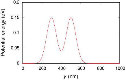
Figure 2: Potential energy considered in the armchair ribbon.

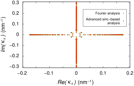
Figure 3: Position on the Gauss plane of all the longitudinal wave vectors $\kappa_{x}$ obtained with the Fourier analysis and with our advanced sinc-based approach.

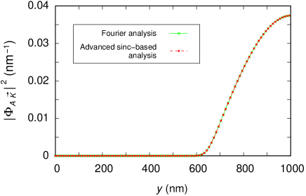
Figure 4: Envelope function $\Phi_{A\vec{K}}(y)$ corresponding to the eigenvalue with the largest real part, computed with a Fourier analysis and with our advanced sinc-based approach.

Figure 5: Position on the Gauss plane of all the longitudinal wave vectors $\kappa_{x}$ obtained with the simplified sinc-based approach. The highest order wave vectors strongly differ from those obtained with a Fourier analysis (see Fig. 3).

For example, we have considered a potential $U(y)$ (represented in Fig. 2) equal to the sum of two Gaussian functions:

$$U(y)=0.15~{}{\rm eV}\cdot e^{-\frac{\scriptstyle(y-300\>{\rm nm})^{2}}{\scriptstyle 5000\>{\rm nm}^{2}}}+0.15~{}{\rm eV}\cdot e^{-\frac{\scriptstyle(y-500\>{\rm nm})^{2}}{\scriptstyle 5000\>{\rm nm}^{2}}}$$ (43)

in a 8131 dimer line ($\sim$1 $\mu$m) wide armchair nanoribbon, considering an electron injection energy $E=0.1$ eV. In Figs. 3 and 4, we show the results that we have obtained considering $N=99$ and $M=21$ with the advanced approach in the direct space, and we compare them with those achieved by means of a Fourier analysis. In particular, in Fig. 3, we show the position on the Gauss plane of all the obtained longitudinal wave vectors $\kappa_{x}$; and in Fig. 4, we represent the behavior of the envelope function $\Phi_{A\vec{K}}(y)$ corresponding to the eigenvalue with the largest real part. As expected, the two methods yield exactly the same results.

Instead, in Fig. 5, we show the values of the longitudinal wave vectors $\kappa_{x}$ obtained with the simplified treatment of the product term. As we can see from the highest order wave vectors, this method is not equivalent to the Fourier one, even though it yields quite good results for the low-order modes.

VII Conclusion

We have proposed a method, based on a set of basis functions resulting from the periodic repetition of sinc functions, for the numerical solution, in the direct space, of differential problems and, in particular, of quantum wave equations, with periodic boundary conditions.

This approach is equivalent to a Fourier analysis and (once we have chosen a given discretization) requires the solution of a linear system with the same matrix size. It allows performing a very efficient solution in the direct space, without the need to Fourier transform the input functions and finally to inverse transform the solutions.

We have applied this method to efficiently solve the Dirac equation in an armchair graphene nanoribbon in the direct space, verifying its equivalence to a reciprocal space approach.

We believe that this treatment also helps in clarifying the exact origin of the differences in the convergence behavior observed between direct space and reciprocal space approaches.

Appendix A Orthonormality of the basis functions

The orthonormality of two sinc functions centered on different sampling points can be easily demonstrated in the following way:

$$\displaystyle\int_{-\infty}^{+\infty}{\rm sinc}\left(\frac{x-j\Delta}{\Delta}\right){\rm sinc}\left(\frac{x-\ell\Delta}{\Delta}\right)\,dx$$

$$\displaystyle=\left[{\rm sinc}\left(\frac{x}{\Delta}\right)\ast{\rm sinc}\left(\frac{x}{\Delta}\right)\right]_{x=(\ell-j)\Delta}$$

$$\displaystyle=\left\{\mathcal{F}^{-1}\left[\Delta^{2}{\rm rect}(\Delta f)\right]\right\}_{x=(\ell-j)\Delta}$$

$$\displaystyle=\Delta\,{\rm sinc}(\ell-j)=\Delta\,\delta_{j,\ell}\,,$$ (44)

where $\ast$ is the convolution operator and $\mathcal{F}^{-1}$ is the inverse Fourier transform.

Moreover, if the function $z(x)$ is periodic with period $L$, we have that

$$\displaystyle\frac{1}{\Delta}\int_{0}^{L}g_{j,\Delta}^{*}(\chi)z(\chi)\,d\chi=\frac{1}{\Delta}\int_{0}^{L}g_{j,\Delta}(\chi)z(\chi)\,d\chi$$

$$\displaystyle=\frac{1}{\Delta}\sum_{\eta=-\infty}^{+\infty}\int_{0}^{L}{\rm sinc}\left(\frac{\chi-(j+\eta N)\Delta}{\Delta}\right)z(\chi)\,d\chi$$

$$\displaystyle=\frac{1}{\Delta}\sum_{\eta=-\infty}^{+\infty}\int_{-\eta L}^{(-\eta+1)L}{\rm sinc}\left(\frac{\xi-j\Delta}{\Delta}\right)z(\xi+\eta N\Delta)\,d\xi$$

$$\displaystyle=\frac{1}{\Delta}\sum_{\eta=-\infty}^{+\infty}\int_{-\eta L}^{(-\eta+1)L}{\rm sinc}\left(\frac{\xi-j\Delta}{\Delta}\right)z(\xi)\,d\xi$$

$$\displaystyle=\frac{1}{\Delta}\int_{-\infty}^{+\infty}{\rm sinc}\left(\frac{\xi-j\Delta}{\Delta}\right)z(\xi)\,d\xi\,,$$ (45)

where we have changed the integration variable from $\chi$ to $\xi=\chi-\eta N\Delta=\chi-\eta L$.

From the previous observation, we derive the orthonormality of the $g$ functions

$$\displaystyle\frac{1}{\Delta}\int_{0}^{L}g_{j,\Delta}^{*}(x)g_{\ell,\Delta}(x)\,dx\qquad\qquad\qquad\qquad\qquad\qquad\qquad$$

$$\displaystyle=\frac{1}{\Delta}\int_{-\infty}^{+\infty}{\rm sinc}\left(\frac{\xi-j\Delta}{\Delta}\right)g_{\ell,\Delta}(x)\,d\xi$$

$$\displaystyle=\frac{1}{\Delta}\sum_{\eta=-\infty}^{+\infty}\int_{-\infty}^{+\infty}{\rm sinc}\left(\frac{\xi-j\Delta}{\Delta}\right){\rm sinc}\left(\frac{x-(\ell+\eta N)\Delta}{\Delta}\right)$$

$$\displaystyle=\frac{1}{\Delta}\sum_{\eta=-\infty}^{+\infty}\Delta\,\delta_{j,\ell+\eta N}=\sum_{\eta=-\infty}^{+\infty}\delta_{j,\ell}\,\delta_{\eta,0}=\delta_{j,\ell}\qquad\qquad\qquad$$ (46)

(with $j,\ell=0,\ldots,N-1$).

Appendix B Notes on the product term

Operating in the reciprocal space, if we substitute

$$\varphi(x)=\sum_{r=-D}^{D}a_{r}e^{i2\pi r\frac{\scriptstyle x}{\scriptstyle L}}\,,\quad\tilde{f}(x)=\sum_{q=-Q}^{Q}f_{q}e^{i2\pi q\frac{\scriptstyle x}{\scriptstyle L}}$$ (47)

(with $f_{q}$ being the DFT coefficients of $f(x)$ computed on its $N\,M=2\,Q+1$ samples) into the term $h(x)=\tilde{f}(x)\varphi(x)$ and then we consider only the frequency components of the product within the interval $[-D/L,D/L]$, we obtain that

$$h_{0}(x)=\underset{|q+r|\leq D}{\sum_{q=-Q}^{Q}\,\sum_{r=-D}^{D}}f_{q}a_{r}e^{i2\pi(q+r)\frac{\scriptstyle x}{\scriptstyle L}}=\underset{|p-r|\leq Q}{\sum_{p=-D}^{D}\,\sum_{r=-D}^{D}}f_{p-r}a_{r}e^{i2\pi p\frac{\scriptstyle x}{\scriptstyle L}}\,.$$ (48)

Since the functions $\exp(i2\pi px/L)$ with $|p|\leq D$ are band limited with band $B\leq 1/(2\Delta)$, they can be expressed in terms of their samples taken with sampling interval $\Delta$

$$e^{i2\pi p\frac{\scriptstyle x}{\scriptstyle L}}=\sum_{\mu=0}^{N-1}e^{i2\pi p\frac{\scriptstyle\mu}{\scriptstyle N}}\,g_{\mu,\Delta}(x)\,.$$ (49)

Moreover, exploiting Eq. (27), the coefficients $a_{r}$ and $f_{p-r}$ can be replaced with

$$a_{r} = \frac{1}{N}\sum_{\ell=0}^{N-1}\varphi(\ell\,\Delta)\,e^{-i2\pi r\frac{\scriptstyle\ell}{\scriptstyle N}}\,,$$

$$f_{p-r} = \frac{1}{MN}\sum_{m=0}^{MN-1}f(m\,\Delta^{\prime})\,e^{-i2\pi(p-r)\frac{\scriptstyle m}{\scriptstyle MN}}\,.$$ (50)

After these substitutions, we obtain that

$$h_{0}(x)=\sum_{\mu=0}^{N-1}\left[\sum_{\ell=0}^{N-1}\varphi(\ell\,\Delta)\beta_{\mu\ell}\right]g_{\mu,\Delta}(x)$$ (51)

with

$$\beta_{\mu\ell}=\frac{1}{MN^{2}}\sum_{m=0}^{MN-1}f\left(m\,\Delta^{\prime}\right)\nu_{\mu\ell m}$$ (52)

and

$$\nu_{\mu\ell m} = \displaystyle\underset{|p-r|\leq Q}{\sum_{p=-D}^{D}\,\sum_{r=-D}^{D}}\left[e^{i\frac{\scriptstyle 2\pi}{\scriptstyle N}\left(\mu-\frac{\scriptstyle m}{\scriptstyle M}\right)}\right]^{p}\left[e^{i\frac{\scriptstyle 2\pi}{\scriptstyle N}\left(\ell-\frac{\scriptstyle m}{\scriptstyle M}\right)}\right]^{-r}$$ (53)

$$= \displaystyle\underset{|p+\tilde{r}|\leq Q}{\sum_{p=-D}^{D}\,\sum_{\tilde{r}=-D}^{D}}\left[e^{i\frac{\scriptstyle 2\pi}{\scriptstyle N}\left(\mu-\frac{\scriptstyle m}{\scriptstyle M}\right)}\right]^{p}\left[e^{i\frac{\scriptstyle 2\pi}{\scriptstyle N}\left(\ell-\frac{\scriptstyle m}{\scriptstyle M}\right)}\right]^{\tilde{r}}$$

(with $\tilde{r}=-r$).

Equations (51) and (52) coincide with Eqs. (16)–(18) obtained operating in the direct space. We can prove that Eq. (53) coincides with Eq. (19), too. In detail, using Eq. (26), we can write the Fourier expansion of the $g$ functions as follows:

$$\displaystyle g_{\mu,\Delta}(x)=\frac{1}{N}\sum_{p=-D}^{D}e^{i2\pi p\frac{\scriptstyle x-\mu\Delta}{\scriptstyle L}}\,,$$ (54)

$$\displaystyle g_{m,\Delta^{\prime}}(x)=\frac{1}{MN}\sum_{q=-Q}^{Q}e^{i2\pi q\frac{\scriptstyle x-m\Delta^{\prime}}{\scriptstyle L}}\,,$$ (55)

$$\displaystyle g_{\ell,\Delta}(x)=\frac{1}{N}\sum_{r=-D}^{D}e^{i2\pi r\frac{\scriptstyle x-\ell\Delta}{\scriptstyle L}}\,.$$ (56)

Substituting Eqs. (54)–(56) into Eq. (19), we find that

$$\nu_{\mu\ell m} = \displaystyle\frac{1}{\Delta}\frac{1}{N}\sum_{p=-D}^{D}\,\sum_{q=-Q}^{Q}\,\sum_{r=-D}^{D}e^{i\frac{\scriptstyle 2\pi}{\scriptstyle N}\left(p\mu-\frac{\scriptstyle qm}{\scriptstyle M}-r\ell\right)}L\delta_{q,p-r}$$ (57)

$$= \displaystyle\underset{|p-r|\leq Q}{\sum_{p=-D}^{D}\,\sum_{r=-D}^{D}}\left[e^{i\frac{\scriptstyle 2\pi}{\scriptstyle N}\left(\mu-\frac{\scriptstyle m}{\scriptstyle M}\right)}\right]^{p}\left[e^{i\frac{\scriptstyle 2\pi}{\scriptstyle N}\left(\ell-\frac{\scriptstyle m}{\scriptstyle M}\right)}\right]^{-r},$$

which coincides with Eq. (53).

If $M>1$, the condition $|p-r|\leq Q$ (i.e., $|p+\tilde{r}|\leq Q$) is always satisfied and thus

$$\nu_{\mu\ell m}=\sum_{p=-D}^{D}\left[e^{i\frac{\scriptstyle 2\pi}{\scriptstyle N}\left(\mu-\frac{\scriptstyle m}{\scriptstyle M}\right)}\right]^{p}\sum_{\tilde{r}=-D}^{D}\left[e^{i\frac{\scriptstyle 2\pi}{\scriptstyle N}\left(\ell-\frac{\scriptstyle m}{\scriptstyle M}\right)}\right]^{\tilde{r}}=\lambda_{1}(m,\mu)\lambda_{1}(m,\ell)\,,$$ (58)

which corresponds to Eq. (20).

Instead, if $M=1$, the condition $|p+\tilde{r}|\leq Q$ has to be taken into consideration. From Eq. (53), we see that for each value of $p$, we have to sum over the integers $\tilde{r}$ for which $-D\leq\tilde{r}\leq D$ and $-p-D\leq\tilde{r}\leq-p+D$ (note that $Q=D$ if $M=1$). This set of values of $\tilde{r}$ corresponds for $p=0$ to $-D\leq\tilde{r}\leq D$, for $p>0$ to $-D\leq\tilde{r}\leq-p+D$, and for $p<0$ to $-p-D\leq\tilde{r}\leq D$. Therefore, Eq. (53) can be rewritten in the following way:

$$\nu_{\mu\ell m} = \displaystyle\sum_{\tilde{r}=-D}^{D}\left[e^{i\frac{\scriptstyle 2\pi}{\scriptstyle N}(\ell-m)}\right]^{\tilde{r}}$$

$$+ \displaystyle\sum_{p=1}^{D}\Bigg{\{}\left[e^{i\frac{\scriptstyle 2\pi}{\scriptstyle N}(\mu-m)}\right]^{p}\sum_{\tilde{r}=-D}^{-p+D}\left[e^{i\frac{\scriptstyle 2\pi}{\scriptstyle N}(\ell-m)}\right]^{\tilde{r}}\Bigg{\}}$$

$$+ \displaystyle\sum_{p=-D}^{-1}\Bigg{\{}\left[e^{i\frac{\scriptstyle 2\pi}{\scriptstyle N}(\mu-m)}\right]^{p}\sum_{\tilde{r}=-p-D}^{D}\left[e^{i\frac{\scriptstyle 2\pi}{\scriptstyle N}(\ell-m)}\right]^{\tilde{r}}\Bigg{\}}\,.$$

Computing the first sum and noting that the third sum is the complex conjugate of the second one, we can rewrite this expression as:

$$\nu_{\mu\ell m}=N\delta_{m,\ell}+2\,{\rm Re}\Bigg{\{}\sum_{p=1}^{D}\bigg{\{}\left[e^{i\frac{\scriptstyle 2\pi}{\scriptstyle N}(\mu-m)}\right]^{p}\sum_{\tilde{r}=-D}^{-p+D}\left[e^{i\frac{\scriptstyle 2\pi}{\scriptstyle N}(\ell-m)}\right]^{\tilde{r}}\bigg{\}}\Bigg{\}}\,.$$ (60)

If $\ell=m$, this is equal to

$$\nu_{\mu\ell m}=N+2\,{\rm Re}\left\{\sum_{p=1}^{D}\left\{\left[e^{i\frac{\scriptstyle 2\pi}{\scriptstyle N}(\mu-m)}\right]^{p}(N-p)\right\}\right\}=\lambda_{2}(m,\mu)\,.$$ (61)

If $\ell\neq m$ instead, we have that

$$\displaystyle\nu_{\mu\ell m} = \displaystyle 2\,{\rm Re}\Bigg{\{}\sum_{p=1}^{D}\bigg{\{}\left[e^{i\frac{\scriptstyle 2\pi}{\scriptstyle N}(\mu-m)}\right]^{p}\frac{\displaystyle(-1)^{\ell-m}}{\displaystyle 2i\sin\left(\frac{\pi}{N}\,(\ell-m)\right)}\left[e^{-i\frac{\scriptstyle 2\pi}{\scriptstyle N}p(\ell-m)}-1\right]\bigg{\}}\Bigg{\}}$$ (62)

$$= \displaystyle\frac{\displaystyle(-1)^{\ell-m}}{\displaystyle\sin\left(\frac{\pi}{N}\,(\ell-m)\right)}\Bigg{[}{\rm Im}\bigg{\{}\sum_{p=1}^{D}\left[e^{i\frac{\scriptstyle 2\pi}{\scriptstyle N}(\mu-\ell)}\right]^{p}\bigg{\}}-{\rm Im}\bigg{\{}\sum_{p=1}^{D}\left[e^{i\frac{\scriptstyle 2\pi}{\scriptstyle N}(\mu-m)}\right]^{p}\bigg{\}}\Bigg{]}$$

$$= \frac{\displaystyle(-1)^{\ell-m}\,\left(\lambda_{3}(\ell,\mu)-\lambda_{3}(m,\mu)\right)}{\displaystyle\sin\left(\frac{\pi}{N}\,(\ell-m)\right)}\,.$$

Equations (61) and (62) correspond to Eq. (22).

References

- (1) R. Stacey, Phys. Rev. D 26, 468 (1982).
- (2) C. M. Bender, K. A. Milton and D. H. Sharp, Phys. Rev. Lett. 51, 1815 (1983).
- (3) L. Susskind, Phys. Rev. D 16, 3031 (1977).
- (4) K. S. Novoselov, A. K. Geim, S. V. Morozov, D. Jiang, Y. Zhang, S. V. Dubonos, I. V. Grigorieva and A. A. Firsov, Science 306, 666 (2004).
- (5) A. K. Geim and K. S. Novoselov, Nature Mater. 6, 183 (2007).
- (6) A. K. Geim, Science 324, 1530 (2009).
- (7) A. H. Castro Neto, F. Guinea, N. M. R. Peres, K. S. Novoselovand A. K. Geim, Rev. Mod. Phys. 81, 109 (2009).
- (8) D. R. Cooper, B. D’Anjou, N. Ghattamaneni, B. Harack, M. Hilke, A. Horth, N. Majlis, M. Massicotte, L. Vandsburger, E. Whiteway and V. Yu, “Experimental Review of Graphene,” ISRN Condensed Matter Physics 2012, art. number 501686 (2012).
- (9) S. Mikhailov, Physics and Applications of Graphene (InTech, Rijeka, 2011).
- (10) M. R. Connolly, R. K. Puddy, D. Logoteta, P. Marconcini, M. Roy, J. P. Griffiths, G. A. C. Jones, P. A. Maksym, M. Macucci and C. G. Smith, Nano Lett. 12, 5448 (2012).
- (11) D. Logoteta, P. Marconcini, M. R. Connolly, C. G. Smith and M. Macucci, “Numerical simulation of scanning gate spectroscopy in bilayer graphene in the Quantum Hall regime,” in Proceedings of IWCE 2012 (IEEE Conference Proceedings) (2012), art. number 6242841, DOI: 10.1109/IWCE.2012.6242841.
- (12) P. Marconcini, A. Cresti, F. Triozon, G. Fiori, B. Biel, Y.-M. Niquet, M. Macucci and S. Roche, ACS Nano 6, 7942 (2012).
- (13) P. Marconcini, A. Cresti, F. Triozon, G. Fiori, B. Biel, Y.-M. Niquet, M. Macucci and S. Roche, “Electron-hole transport asymmetry in Boron-doped Graphene Field Effect Transistors,” in Proceedings of IWCE 2012 (IEEE Conference Proceedings) (2012), art. number 6242844, DOI: 10.1109/IWCE.2012.6242844.
- (14) H. Raza, Graphene Nanoelectronics: Metrology, Synthesis, Properties and Applications (Springer, Heidelberg, 2012).
- (15) F. Schwierz, Nature Nanotech. 5, 487 (2010).
- (16) G. Iannaccone, G. Fiori, M. Macucci, P. Michetti, M. Cheli, A. Betti and P. Marconcini, “Perspectives of graphene nanoelectronics: probing technological options with modeling,” in Proceedings of IEDM 2009 (IEEE Conference Proceedings) (2009), p. 245, DOI: 10.1109/IEDM.2009.5424376.
- (17) P. Y. Yu and M. Cardona, Fundamentals of Semiconductors (Springer, Heidelberg, 2003).
- (18) V. Mitin, V. Kochelap and M. A. Stroscio, Quantum Heterostructures. Microelectronics and Optoelectronics (Cambridge University Press, Cambridge, 1999).
- (19) P. Marconcini, M. Macucci, G. Iannaccone, B. Pellegrini and G. Marola, Europhys. Lett. 73, 574 (2006).
- (20) R. S. Whitney, P. Marconcini and M. Macucci, Phys. Rev. Lett. 102, 186802 (2009).
- (21) P. Marconcini, M. Macucci, G. Iannaccone and B. Pellegrini, Phys. Rev. B 79, 241307(R) (2009).
- (22) P. Marconcini, M. Macucci, D. Logoteta and M. Totaro, Fluct. Noise Lett. 11, 1240012 (2012).
- (23) P. Marconcini, M. Totaro, G. Basso and M. Macucci, AIP Advances 3, 062131 (2013).
- (24) T. Ando, J. Phys. Soc. Jpn. 74, 777 (2005).
- (25) P. Marconcini and M. Macucci, “The kp method and its application to graphene, carbon nanotubes and graphene nanoribbons: the Dirac equation,” La Rivista del Nuovo Cimento 34, 489 (2011).
- (26) J. Tworzydło, C. W. Groth and C. W. J. Beenakker, Phys. Rev. B 78, 235438 (2008).
- (27) A. R. Hernández and C. H. Lewenkopf, Phys. Rev. B 86, 155439 (2012).
- (28) I. Snyman, J. Tworzydło, C. W. J. Beenakker, Phys. Rev. B 78, 045118 (2008).
- (29) D. Logoteta, P. Marconcini and M. Macucci, “Numerical simulation of shot noise in disordered graphene,” in Proceedings of ICNF 2013 (IEEE Conference Proceedings) (2013), art. number 6578889, DOI: 10.1109/ICNF.2013.6578889.
- (30) S. Haykin, An Introduction to Analog and Digital Communications (Wiley, New York, 1989).
- (31) S. Datta, Quantum Phenomena (Addison-Wesley, Reading, Massachussets, 1989).
- (32) C. Canuto, M. Y. Hussaini, A. Quarteroni and T. A. Zang, Spectral Methods: Fundamentals in Single Domains (Springer, Berlin, 2006).
- (33) S. D. Drell, M. Weinstein and S. Yankielowicz, Phys. Rev. D 14, 1627 (1976).
- (34) J. Förster, A. Saenz and U. Wolff, Phys. Rev. E 86, 016701 (2012).
- (35) M. Fagotti, C. Bonati, D. Logoteta, P. Marconcini and M. Macucci, Phys. Rev. B 83, 241406(R) (2011).
- (36) P. Marconcini, D. Logoteta, M. Fagotti and M. Macucci, “Numerical solution of the Dirac equation for an armchair graphene nanoribbon in the presence of a transversally variable potential,” in Proceedings of IWCE 2010 (IEEE Conference Proceedings) (2010), p. 53, DOI: 10.1109/IWCE.2010.5677938.