Emergence of Quantum Mechanics from a Sub-Quantum Statistical Mechanics

Abstract

A research program within the scope of theories on “Emergent Quantum Mechanics” is presented, which has gained some momentum in recent years. Via the modeling of a quantum system as a non-equilibrium steady-state maintained by a permanent throughput of energy from the zero-point vacuum, the quantum is considered as an emergent system. We implement a specific “bouncer-walker” model in the context of an assumed sub-quantum statistical physics, in analogy to the results of experiments by Couder’s group on a classical wave-particle duality. We can thus give an explanation of various quantum mechanical features and results on the basis of a “21^st century classical physics”, such as the appearance of Planck’s constant, the Schrödinger equation, etc. An essential result is given by the proof that averaged particle trajectories’ behaviors correspond to a specific type of anomalous diffusion termed “ballistic” diffusion on a sub-quantum level.

It is further demonstrated both analytically and with the aid of computer simulations that our model provides explanations for various quantum effects such as double-slit or n-slit interference. We show the averaged trajectories emerging from our model to be identical to Bohmian trajectories, albeit without the need to invoke complex wave functions or any other quantum mechanical tool. Finally, the model provides new insights into the origins of entanglement, and, in particular, into the phenomenon of a “systemic” nonlocality.

1 Introduction

After many attempts to frame wave-particle duality on a single “basic” explanatory level, like on pure formalism (Heisenberg,…), pure wave mechanics (de Broglie,…), or pure particle physics (Feynman,…), for example, it is instructive to ask the following question: is perhaps the quantum a more complex dynamical phenomenon? One motivation for raising this question comes from the fact that we are presently witnessing a historical change with respect to wave-particle duality in double-slit interference. With regard to the latter, the standard attitude during practically the whole of the 20th century can be characterized by Richard Feynman’s famous claim that it is “… a phenomenon which is impossible, absolutely impossible to explain in any classical way.” In the present, however, we are facing the beautiful experiments by Yves Couder’s group in Paris which do show wave-particle duality in a completely classical system, i.e., with the aid of bouncers/walkers on an oscillating fluid. (For a first impression, see the video with Yves Couder Couder.2011yves .)

In fact, with our approach we have in a series of papers obtained from a “classical” dynamical model several essential elements of quantum theory Groessing.2008vacuum ; Groessing.2009origin ; Groessing.2010emergence ; Groessing.2011dice ; Groessing.2011explan ; Groessing.2012doubleslit ; Grossing.2012quantum . They derive from the assumption that a “particle” of energy $E=\hbar\omega$ is actually an oscillator of angular frequency $\omega$ phase-locked with the zero-point oscillations of the surrounding environment, the latter of which containing both regular and fluctuating components and being constrained by the boundary conditions of the experimental setup via the buildup and maintenance of standing waves. The “particle” in this approach is an off-equilibrium steady-state maintained by the throughput of zero-point energy from its “vacuum” surroundings. In other words, in our model a quantum emerges from the synchronized dynamical coupling between a bouncer and its wave-like environment. This is in close analogy to the bouncing/walking droplets in the experiments of Couder’s group Couder.2005 ; Couder.2006single-particle ; Couder.2010walking ; Couder.2012probabilities , which in many respects can serve as a classical prototype guiding our intuition. Our research program thus pertains to the scope of theories on “Emergent Quantum Mechanics”. (For the proceedings of a first international conference exclusively devoted to this topic, see Grössing (2012) Groessing.2012emerqum11-book . For their original models, see in particular the papers by Adler, Elze, Ord, Grössing et al., Cetto et al., Hiley, de Gosson, Bacciagaluppi, Budiyono, Schuch, Faber, Hofer, ’t Hooft, Khrennikov et al., Wetterich, and Burinskii.) We have recently applied our model to the case of interference at a double slit Groessing.2012doubleslit , thereby obtaining the exact quantum mechanical probability distributions on a screen behind the double slit, the average particle trajectories (which because of the averaging are shown to be identical to the Bohmian ones), and the involved probability density currents.

Moreover, already some decades ago, Aharonov et al. Aharonov.1969modular ; Aharonov.1970deterministic investigated the problem of double-slit interference “from a single particle perspective”. Their explanation is based on what they call dynamical nonlocality, and they therewith answer the question of how a particle going through one slit can “know” about the state of the other slit (i.e., being open or closed, for example). This type of “dynamical” nonlocality may lead to (causality preserving) changes in probability distributions and is thus distinguished from the kinematic nonlocality implicit in many quantum correlations, which, however, does not cause any changes in probability distributions. Chapter 3 of the present review extends the applicability also of our model to a such a “dynamical” scenario, which in our terminology rather relates to a “systemic” nonlocality, as shall be explicated below.

This paper is organized as follows. In Chapter 2, some main results of our sub-quantum approach to quantum mechanics are presented. We begin by constructing from classical physics a model that explains the quantum mechanical dispersion of a Gaussian wave packet. As a consequence, we obtain the total velocity field for the current emerging from a Gaussian slit, which can easily be extended to a two-slit (and in fact to any n-slit) system, thereby also providing an explanation of the famous interference effects. With the thus obtained velocity field, one can by integration also obtain an action function that generalizes the ordinary classical one to the case that is relevant for the reproduction of the quantum results. Effectively, this is achieved by the appearance of an additional kinetic energy term, which we associate with fluxes of “heat” in the vacuum, i.e., sub-quantum currents based on the existence of the zero-point energy field. Finally, it is shown how the Schrödinger equation can be derived in a straightforward manner from the said generalized action function, or the corresponding Lagrangian, respectively. In Chapter 3, then, we deal with the above-mentioned problem of interference from the single particle perspective, obtaining results which are in agreement with those presented by Aharonov et al. Aharonov.1969modular ; Aharonov.1970deterministic , but differing in interpretation. Finally, in Chapter 4 computer simulations are presented to show some examples of how our sub-quantum approach reproduces results of ordinary quantum mechanics, but eventually may go beyond these.

2 The Quantum as an Emergent System: A Sub-Quantum Approach to Quantum Mechanics

We transfer an insight from the Couder experiments into our modeling of quantum systems and assume that the waves are a space-filling phenomenon involving the whole experimental setup. Thus, one can imagine a partial decoupling of the physics of waves and particles in that the latter still may be “guided” through said “landscape”, but the former may influence other regions of the “landscape” by providing specific phase information independently of the propagation of the particle. This is why a remote change in the experimental setup, when mediated to the particle via de- and/or re-construction of standing waves, can amount to a nonlocal effect on a particle via the thus modified guiding landscape.

In earlier work Groessing.2010emergence we presented a model for the classical explanation of the quantum mechanical dispersion of a free Gaussian wave packet. In accordance with the classical model, we now relate it more directly to a “double solution” analogy gleaned from Couder and Fort Couder.2012probabilities . These authors used the double solution ansatz to describe the behaviors of their “bouncer”- (or “walker”-) droplets: on an individual level, one observes particles surrounded by circular waves they emit through the phase-coupling with an oscillating bath, which provides, on a statistical level, the emergent outcome in close analogy to quantum mechanical behavior (like, e.g., diffraction or double-slit interference). Originally, the expression of a “double solution” refers to an early idea of de Broglie DeBroglie.1960book to model quantum behavior by a two-fold process, i.e., by the movement of a hypothetical point-like “singularity solution” of the Schrödinger equation, and by the evolution of the usual wavefunction that would provide the empirically confirmed statistical predictions. Now, it is interesting to observe that one can construct various forms of classical analogies to the quantum mechanical Gaussian dispersion Holland.1993 , and one of them even can be related to the double solution idea.

To establish correlations on a statistical level between individual uncorrelated particle positions $x$ and momenta $p$, respectively, one considers a solution of the free Liouville equation providing a certain phase-space distribution $f\left(x,p,t\right)$. This distribution shows the emergence of correlations between $x$ and $p$ from an initially uncorrelated product function of non-spreading (“classical”) Gaussian position distributions as well as momentum distributions. The motivation for their introduction comes exactly from what one observes in the Couder experiments. In an idealized scenario, we assume that at each point $x$ an unbiased emission of momentum fluctuations $\pi_{0}$ in all possible directions takes place, thus mimicking (in a two-dimensional scenario) the circular waves emitted from the “particle as bouncer”. If we compare the typical frequency of the bouncers in the Couder experiments (i.e., roughly $10^{2}\mathrm{\,Hz}$) with that of an electron, for example (i.e., roughly $10^{20}\,\mathrm{Hz}$), we see that a “continuum ansatz” is very pragmatical, particularly if we are interested in statistical averages over a long series of experimental runs.

Thus, one can construct said phase-space distribution, with $\sigma_{0}$ being the initial $x$–space standard deviation, i.e., $\sigma_{0}=\sigma(t=0)$, and $\pi_{0}:=mu_{0}$ the momentum standard deviation, such that

$$f\left(x,p,t\right)=\frac{1}{2\pi\sigma_{0}mu_{0}}\exp\left\{-\frac{\left(x-pt/m\right)^{2}}{2\sigma_{0}^{2}}\right\}\exp\left\{-\frac{p^{2}}{2m^{2}u_{0}^{2}}\right\}.$$ (2.1)

Now, the above-mentioned correlations between $x$ and $p$ emerge when one considers the probability density in $x$–space. Integration over $p$ provides

$$P\left(x,t\right)=\int f\,\mathrm{d}p=\frac{1}{\sqrt{2\pi}\sigma}\exp\left\{-\frac{x^{2}}{2\sigma^{2}}\right\},$$ (2.2)

with the standard deviation at time $t$ given by

$$\sigma^{2}=\sigma_{0}^{2}+u_{0}^{2}\,t^{2}.$$ (2.3)

In other words, the distribution (2.2) with property (2.3) describes a spreading Gaussian which is obtained from a continuous set of classical, i.e., non-spreading, Gaussian position distributions of particles whose associated momentum fluctuations also have non-spreading Gaussian distributions. One thus obtains the exact quantum mechanical dispersion formula for a Gaussian, as we have obtained also previously from a different variant of our classical ansatz. For confirmation with respect to the latter (diffusion-based) model Groessing.2010emergence ; Groessing.2011dice , we consider with (2.2) the usual definition of the “osmotic” velocity field, which in this case yields $u=-D\frac{\nabla P}{P}=\frac{xD}{\sigma^{2}}$. One then obtains, with bars denoting averages over fluctuations and positions, i.e., with $\overline{x^{2}}=\int Px^{2}dx=\sigma^{2}$,

$$\overline{u^{2}}=D^{2}\overline{\left(\frac{\nabla P}{P}\right)^{2}}=D^{2}\int P\left(\frac{\nabla P}{P}\right)^{2}\,\mathrm{d}x=\frac{D^{2}}{\sigma^{2}},\;\;\textrm{and thus also}\;\;u_{0}=\frac{D}{\sigma_{0}},$$ (2.4)

so that one can rewrite Eq. (2.3) in the more familiar form

$$\sigma^{2}=\sigma_{0}^{2}\left(1+\frac{D^{2}t^{2}}{\sigma_{0}^{4}}\right).$$ (2.5)

Note also that by using the Einstein relation $D=\hbar/2m=h/4\pi m$ the norm in (2.1) thus becomes the invariant expression (reflecting the “exact uncertainty relation” Hall.2002schrodinger )

$$\frac{1}{2\pi\sigma_{0}mu_{0}}=\frac{1}{2\pi mD}=\frac{2}{h}.$$ (2.6)

Following from (2.5), in Grössing et al. Groessing.2010emergence ; Groessing.2012doubleslit we obtained for “smoothed-out” trajectories (i.e., averaged over a very large number of Brownian motions) a sum over a deterministic and a fluctuations term, respectively, for the motion in the $x$–direction

$$x_{{\rm tot}}(t)=vt+x(t)=vt+x(0)\frac{\sigma}{\sigma_{0}}=vt+x(0)\sqrt{1+\frac{D^{2}t^{2}}{\sigma_{0}^{4}}}.$$ (2.7)

Thus one classically obtains with $x\left(t\right)=x_{{\rm tot}}(t)-vt$ the average velocity field of a Gaussian wave packet as

$$v_{{\rm tot}}(t)=v(t)+\frac{\,\mathrm{d}x(t)}{{\rm\,\mathrm{d}t}}=v(t)+\left[x(t)\right]\frac{u_{0}^{2}t}{\sigma^{2}}.$$ (2.8)

For the particular choice of $x\left(t\right)=\sigma$, then, and with $\frac{\sigma}{t}\rightarrow u_{0}$ for $t\rightarrow\infty$, one obtains for large $t$ that $v_{{\rm tot}}(t)=v(t)+u_{0}$.

Note that Eqs. (2.7) and (2.8) are derived solely from statistical physics. Still, they are in full accordance with quantum theory, and in particular with Bohmian trajectories Holland.1993 . Note also that one can rewrite Eq. (2.5) such that it appears like a linear-in-time formula for Brownian motion,

$$\overline{x^{2}}=\overline{x^{2}(0)}+D_{\mathrm{t}}\,t,$$ (2.9)

where a time dependent diffusivity

$$D_{\mathrm{t}}=u_{0}^{2}\,t=\frac{\hbar^{2}}{4m^{2}\sigma_{0}^{2}}\,t$$ (2.10)

characterizes Eq. (2.9) as ballistic diffusion. This makes it possible to simulate the dispersion of a Gaussian wave packet on a computer by simply employing coupled map lattices for classical diffusion, with the diffusivity given by Eq. (2.10). (For detailed discussions, see Grössing et al. (2010) Groessing.2010emergence and Grössing et al. (2011) Groessing.2011dice and the last Chapter of this paper.)

Moreover, one can easily extend this scheme to more than one slit, like, for example, to explain interference effects at the double slit Groessing.2012doubleslit ; Grossing.2012quantum . For this, we chose similar initial situations as in Holland Holland.1993 , i.e., electrons (represented by plane waves in the forward $y$–direction) from a source passing through “soft-edged” slits $1$ and $2$ in a barrier (located along the $x$–axis) and recorded at a screen. In our model, we therefore note two Gaussians representing the totality of the effectively “heated-up” path excitation field, one for slit $1$ and one for slit $2$, whose centers have the distances $+X$ and $-X$ from the plane spanned by the source and the center of the barrier along the $y$–axis, respectively.

With the total amplitude $R$ of two coherent waves with (suitably normalized) amplitudes $R_{i}=\sqrt{P_{i}}$, and the local phases $\varphi_{i}$, $i=1$ or $2$, one has, according to classical textbook wisdom, the averaged total intensity

$$P_{{\rm tot}}:=R^{2}=R_{1}^{2}+R_{2}^{2}+2R_{1}R_{2}\cos\varphi_{12}=P_{1}+P_{2}+2\sqrt{P_{1}P_{2}}\cos\varphi_{12},$$ (2.11)

where $\varphi_{12}$ is the relative phase $\varphi_{12}=\varphi_{1}-\varphi_{2}=\left(\mathbf{k}_{1}-\mathbf{k}_{2}\right)\cdot\mathbf{r}$. Note that $\varphi_{12}$ enters Eq. (2.11) only via the cosine function, such that, e.g., even if the total wave numbers (and thus also the total momenta) $\mathbf{k}_{i}$ were of vastly different size, the cosine effectively makes Eq. (2.11) independent of said sizes, but dependent only on an angle modulo $2\pi$. This will turn out as essential for our discussion further below.

The $x$–components of the centroids’ motions from the two alternative slits $1$ and $2$, respectively, are given by the “particle” velocity components

$$v_{x}=\pm\frac{\hbar}{m}\,k_{x},$$ (2.12)

respectively, such that the relative group velocity of the Gaussians spreading into each other is given by $\Delta v_{x}=2v_{x}$. However, in order to calculate the phase difference $\varphi_{12}$ descriptive of the interference term of the intensity distribution (2.11), one must take into account the total momenta involved, i.e., one must also include the wave packet dispersion as described above. Thus, one obtains with the displacement $\pm x\left(t\right)=\mp\left(X+v_{x}t\right)$ in Eq. (2.8) the total relative velocity of the two Gaussians as

$$\Delta v_{{\rm tot},x}=2\left[v_{x}-(X+v_{x}t)\frac{u_{0}^{2}t}{\sigma^{2}}\right].$$ (2.13)

Therefore, the total phase difference between the two possible paths 1 and 2 (i.e., through either slit) becomes

$$\varphi_{12}=\frac{1}{\hbar}(m\Delta v_{{\rm tot},x}\,x)=2mv_{x}\frac{x}{\hbar}-(X+v_{x}t)x\frac{1}{D}\frac{u_{0}^{2}t}{\sigma^{2}}.$$ (2.14)

In earlier papers, Grössing (et al.) Groessing.2008vacuum ; Groessing.2009origin ; Groessing.2010emergence , we have shown that, apart from the ordinary particle current $\mathbf{J}(\mathbf{x},t)=P(\mathbf{x},t)\mathbf{v}$, we are now dealing with two additional, yet opposing, currents $\mathbf{J}_{u}=P(\mathbf{x},t)\mathbf{u}$, which are on average orthogonal to $\mathbf{J}$, and which are the emergent outcome from the presence of numerous momentum fluctuations, and the corresponding velocities,

$$\mathbf{u}_{\pm}=\mp\frac{\hbar}{2m}\frac{\nabla P}{P}.$$ (2.15)

We denote with $\mathbf{u}_{+}$ and $\mathbf{u}_{-}$, respectively, the two opposing tendencies of the diffusion process. Moreover, one can also take the averages over fluctuations and positions to obtain a “smoothed-out” average velocity field Groessing.2008vacuum ; Groessing.2009origin ; Groessing.2010emergence ; Groessing.2011dice , i.e.,

$$\overline{\mathbf{u}(\mathbf{x},t)}=\int P\mathbf{u}(\mathbf{x},t)\,\mathrm{d}^{n}x.$$ (2.16)

In effect, the combined presence of the velocity fields $\mathbf{u}$ and $\mathbf{v}$ can be denoted as a path excitation field: via diffusion, the bouncer in its interaction with already existing wave-like excitations of the environment creates an “agitated”, or “heated-up”, thermal landscape, which can also be pictured by interacting wave configurations all along between source and detector of an experimental setup. Recall that our prototype of a “walking bouncer”, i.e., from the experiments of Couder’s group, is always driven by its interactions with a superposition of waves emitted at the points it visited in the past. Couder et al. denote this superposition of in-phase waves the “path memory” of the bouncer Fort.2010path-memory . This implies, however, that the bouncers at the points visited in “the present” necessarily create new wave configurations which will form the basis of a “path memory” in the future. In other words, the wave configurations of the past determine the bouncer’s path in the present, whereas its bounces in the present co-determine the wave configurations, and thus the probability density distribution, at any of the possible locations it will visit in the future. Therefore, by calling the latter configurations a path excitation field, we point to our model’s physical meaning of the probability density distribution: its time evolution is to be understood as the totality of all sub-quantum currents, which may also be described as a “heated-up” thermal field.

For illustration, let us now consider a single, classical “particle” (“bouncer”) following the propagation of a set of waves of equal amplitude $R_{i}$, each representing one of $i$ possible alternatives according to our principle of path excitation, and focus on the specific role of the velocity fields. To describe the required details, each path $i$ be occupied by a Gaussian wave packet with a “forward” momentum $\mathbf{p}_{i}=\hbar\mathbf{k}_{i}=m\mathbf{v}_{i}$. Moreover, due to the stochastic process of path excitation, the latter has to be represented also by a large number $N$ of consecutive Brownian shifts as in Eq. (2.15), which on average, for stretches of free particle propagation $\mathbf{v}_{i}$, are orthogonal to $\mathbf{v}_{i}$. Defining an average total velocity (with indices $i=1$ or $2$ referring to the two slits, and with $+$ and $-$ referring to the right and the left from the average direction of $\mathbf{v}_{i}$, respectively)

$$\overline{\mathbf{v}}_{{\rm tot},i}:=\overline{\mathbf{v}}_{i}+\overline{\mathbf{u}}_{i+}+\overline{\mathbf{u}}_{i-,}$$ (2.17)

with the bars here (and further on, if not declared otherwise) denoting averages only over the spatial directions, we consider two Gaussian probability density distributions, $P_{1}=R_{1}^{2}$ and $P_{2}=R_{2}^{2}$, respectively. Generally, with the total amplitude $R$ of two coherent waves with (suitably normalized) amplitudes $R_{i}=\sqrt{P_{i}}$, and the local phases $\varphi_{i}$, $i=1$ or $2$, one has as usual that

$$R=R_{1}\cos\left(\omega t+\varphi_{1}\right)+R_{2}\cos\left(\omega t+\varphi_{2}\right),$$ (2.18)

which, when squared and averaged, provides the famous formula for the intensity of the interference pattern (2.11). Introducing an arbitrarily chosen unit vector $\mathbf{\hat{n}}$, one may also define $\cos\left(\omega t+\varphi_{i}\left(\mathbf{x}\right)\right)$= $\mathbf{\hat{n}\cdot\mathbf{\hat{k_{i}}\left(\mathbf{x}\mathrm{,t}\right)}},$ such that along with the system’s evolution, the emergent outcome of the time evolution of $R\left(\mathbf{x}\mathrm{,t}\right)$ as a characteristic of our path excitation field can analogously be assumed as

$$R\left(\mathbf{x}\mathrm{,t}\right)=\hat{\mathbf{n}}\cdot\left(R_{1}\mathbf{\hat{k}}_{1}\left(\mathbf{x}\mathrm{,t}\right)+R_{2}\mathbf{\hat{k}}_{2}\left(\mathbf{x}\mathrm{,t}\right)\right).$$ (2.19)

Thus, with regard to the total amplitude $R_{\mathrm{tot}}$ in the double-slit case, one obtains with the appropriate normalization that

$$R_{\mathrm{tot}}^{2}=\left(R_{1}\overline{\hat{\mathbf{v}}}_{{\rm tot},1}+R_{2}\overline{\hat{\mathbf{v}}}_{{\rm tot},2}\right)^{2}.$$ (2.20)

With $P_{\mathrm{tot}}=R_{\mathrm{tot}}^{2}$, one can calculate the time development of the path excitation field, i.e., the spreading out of the total probability density in the form of the total average current $\overline{\mathbf{J}}_{{\rm tot}}=P_{\mathrm{tot}}\overline{\mathbf{v}}_{\mathrm{tot}}$. After a few calculational steps this provides, similarly to Grössing et al. (2012)Groessing.2012doubleslit (but now with slightly different labellings which apply more generally), with the assumed orthogonality $\overline{\mathbf{v}}_{i}\cdot\overline{\mathbf{u}}_{i}=0$ for free particle propagation ($i=1\textrm{ or }2$) that

$$\overline{\mathbf{J}}_{{\rm tot}}=P_{1}\overline{\mathbf{v}}_{1}+P_{2}\overline{\mathbf{v}}_{2}+\sqrt{P_{1}P_{2}}\left(\overline{\mathbf{v}}_{1}+\overline{\mathbf{v}}_{2}\right)\cos\varphi_{12}+\sqrt{P_{1}P_{2}}\left(\overline{\mathbf{u}}_{1}-\overline{\mathbf{u}}_{2}\right)\sin\varphi_{12}.$$ (2.21)

An alternative, more detailed account of Eq. (2.21) and its extension to n slits is in preparation [Fussy et al. (2013)]. Note that Eq. (2.21), upon the identification of $\overline{\mathbf{u}}_{i}=-\frac{\hbar}{m}\frac{\nabla R_{i}}{R_{i}}$ from Eq. (2.15) and with $P_{i}=R_{i}^{2}$, turns out to be in perfect agreement with a comparable “Bohmian” derivation Holland.1993 ; Sanz.2008trajectory . In fact, with $\overline{\mathbf{v}}_{i}=$$\nabla S_{i}$/m, one can rewrite (2.21) as

$$\overline{\mathbf{J}}_{{\rm tot}}= \;R_{1}^{2}\frac{\nabla S_{1}}{m}+R_{2}^{2}\frac{\nabla S_{2}}{m}$$ (2.22)

$$+R_{1}R_{2}\left(\frac{\nabla S_{1}}{m}+\frac{\nabla S_{2}}{m}\right)\cos\varphi_{12}+\frac{\hbar}{m}\left(R_{1}\nabla R_{2}-R_{2}\nabla R_{1}\right)\sin\varphi_{12}.$$

The formula for the averaged particle trajectories, then, simply results from

$$\overline{\mathbf{v}}_{{\rm tot}}=\frac{\overline{\mathbf{J}}_{{\rm tot}}}{P_{\textrm{tot}}}.$$ (2.23)

Although we have obtained the usual quantum mechanical results, we have so far not used the quantum mechanical formalism in any way. However, upon employment of the Madelung transformation for each path $j$ ($j=1$ or $2$),

$$\Psi_{j}=R{\rm e}^{{\rm i}S/\hbar},$$ (2.24)

and thus $P_{j}=R_{j}^{2}=|\Psi_{j}|^{2}=\Psi_{j}^{*}\Psi_{j}$, with the definitions (2.15) and $\overline{v_{j}}:=\nabla S_{j}/m$, $\varphi_{12}=(S_{1}-S_{2})/\hbar$, and recalling the usual trigonometric identities such as $\cos\varphi=\frac{1}{2}\left({\rm e}^{{\rm i}\varphi}+{\rm e}^{-{\rm i}\varphi}\right)$, etc., one can rewrite the total average current (2.21) immediately as

$${\displaystyle\overline{\mathbf{J}}_{{\rm tot}}} =P_{{\rm tot}}\overline{\mathbf{v}}_{{\rm tot}}$$

$$={\displaystyle(\Psi_{1}+\Psi_{2})^{*}(\Psi_{1}+\Psi_{2})\frac{1}{2}\left[\frac{1}{m}\left(-{\rm i}\hbar\frac{\nabla(\Psi_{1}+\Psi_{2})}{(\Psi_{1}+\Psi_{2})}\right)+\frac{1}{m}\left({\rm i}\hbar\frac{\nabla(\Psi_{1}+\Psi_{2})^{*}}{(\Psi_{1}+\Psi_{2})^{*}}\right)\right]}$$

$$={\displaystyle-\frac{{\rm i}\hbar}{2m}\left[\Psi^{*}\nabla\Psi-\Psi\nabla\Psi^{*}\right]={\displaystyle\frac{1}{m}{\rm Re}\left\{\Psi^{*}(-{\rm i}\hbar\nabla)\Psi\right\},}}$$ (2.25)

where $P_{{\rm tot}}=|\Psi_{1}+\Psi_{2}|^{2}=:|\Psi|^{2}$. The last two expressions of (2.25) are the exact well-known formulations of the quantum mechanical probability current, here obtained without any quantum mechanics, but just by a re-formulation of (2.21). In fact, it is a simple exercise to insert the wave functions (2.24) into (2.25) to re-obtain (2.21).

Moreover, having thus obtained a “bridge” to the quantum mechanical formalism, one can now show how the Schrödinger equation not only complies with our classical ansatz, but actually can be derived from it. Two different ways of such a corresponding derivation have already been published by the present author (i.e., one on more general grounds Groessing.2004hamilton , the other within a more concrete model based on nonequilibrium thermodynamicsGroessing.2008vacuum ). Here, however, we just start with a result from the construction of the classical Gaussian with its dispersion mimicking the quantum mechanical one, i.e., more concretely, with the resulting velocity field $v_{{\rm tot}}(t)$ from Eq. (2.8). Integrating the latter, and with $\xi\left(t\right):=x-vt$ describing the location of a particle in a Gaussian probability density distribution $P\left(x,t\right)=\frac{1}{\sqrt{2\pi}\sigma}\exp\left\{-\frac{\left(x-vt\right)^{2}}{2\sigma^{2}}\right\}$, we find an expression for the action function as

$$S =\int mv_{{\rm tot}}(t)\,\mathrm{d}x-\int E\,\mathrm{d}t$$

$$=mvx+\frac{mu_{0}^{2}}{2}\left[\frac{\xi(t)}{\sigma(t)}\right]^{2}t-Et=mvx+\frac{mu_{0}^{2}}{2}\left[\frac{\xi(0)}{\sigma_{0}}\right]^{2}t-Et,$$ (2.26)

with $E$ being the system’s total energy. Note that because it generally holds that $\frac{\xi(t)}{\sigma(t)}=\frac{\xi(0)}{\sigma_{0}}$, the physics contained in (2.26) for the free particle case is essentially determined already by the initial conditions, i.e., where in the Gaussian the particle is initially located. Note also that the new term, as opposed to “ordinary” classical physics, is given by a kinetic energy, which represents a thermal fluctuation field with the kinetic temperature $kT=mu_{0}^{2}\left[\frac{\xi(t)}{\sigma(t)}\right]^{2}$ of what we have termed the path excitation field. Now, as with the above-mentioned Gaussian one has $u\left(x,t\right)=-D\frac{\nabla P}{P}=\frac{\xi(t)D}{\sigma^{2}}=\frac{\xi(t)\sigma_{0}}{\sigma^{2}}u_{0}$, one can rewrite the new kinetic energy term in Eq. (2.26) as

$$\frac{mu_{0}^{2}}{2}\left[\frac{\xi(t)}{\sigma(t)}\right]^{2}t=\frac{mu^{2}}{2}\left[\frac{\sigma(t)}{\sigma_{0}}\right]^{2}t=:\frac{m\tilde{u}^{2}}{2}t,$$ (2.27)

where $\tilde{u}=u\frac{\sigma}{\sigma_{0}}$. (This is therefore in complete accordance with the starting assumption in Grössing (2008) Groessing.2008vacuum .) Moreover, upon averaging over fluctuations and space, one obtains that

$$\int P\frac{mu_{0}^{2}}{2}\left[\frac{\xi(t)}{\sigma(t)}\right]dx=\frac{mu_{0}^{2}}{2}\equiv\frac{\hbar\omega}{2},$$ (2.28)

where the latter equation describes the identity of the averaged kinetic energy term with the zero-point energy as shown in Grössing (2009) Groessing.2009origin .

In more general terms, i.e., independently from the particular choice of $P$ as a Gaussian distribution density, with our expression for the momentum fluctuation $\delta\mathbf{p}=m\mathbf{u}$ as

$$\delta\mathbf{p}(\mathbf{x},t)=\nabla(\delta S(\mathbf{x},t))=-\frac{\hbar}{2}\frac{\nabla P(\mathbf{x},t)}{P(\mathbf{x},t)}\;.$$ (2.29)

we can write our additional kinetic energy term for one particle as

$$\delta E_{{\rm kin}}=\frac{1}{2m}\nabla(\delta S\cdot\nabla(\delta S)=\frac{1}{2m}\left(\frac{\hbar}{2}\frac{\nabla P}{P}\right)^{2}\;.$$ (2.30)

Thus, writing down a classical action integral for $n$ particles, and including this new term for each of them, yields (with Lagrangian $L$ and external potential $V$)

$$A =\int L\,\mathrm{d}^{m}x\,\mathrm{d}t$$

$$=\int P\left[\frac{\partial S}{\partial t}+\sum_{i=1}^{n}\frac{1}{2m_{i}}\nabla_{i}S\cdot\nabla_{i}S+\sum_{i=1}^{n}\frac{1}{2m_{i}}\left(\frac{\hbar}{2}\frac{\nabla_{i}P}{P}\right)^{2}+V\right]\,\mathrm{d}^{m}x\,\mathrm{d}t,$$ (2.31)

where $P=P(\mathbf{x}_{1},\mathbf{x}_{2},\ldots,\mathbf{x}_{n},t)$. Using again the Madelung transformation (2.24) where $R=\sqrt{P}$, one has

$$\overline{\left|\frac{\nabla_{i}\psi}{\psi}\right|^{2}}:=\int\,\mathrm{d}^{m}x\,\mathrm{d}t\left|\frac{\nabla_{i}\psi}{\psi}\right|^{2}=\overline{\left(\frac{1}{2}\frac{\nabla_{i}P}{P}\right)^{2}}+\overline{\left(\frac{\nabla_{i}S}{\hbar}\right)^{2}}\;,$$ (2.32)

and one can rewrite (2.31) as

$$A=\int L\,\mathrm{d}t=\int\,\mathrm{d}^{m}x\,\mathrm{d}t\left[|\psi|^{2}\left(\frac{\partial S}{\partial t}+V\right)+\sum_{i=1}^{n}\frac{\hbar^{2}}{2m_{i}}|\nabla_{i}\psi|^{2}\right]\;.$$ (2.33)

Thus, with the identity $|\psi|^{2}\frac{\partial S}{\partial t}=-\frac{{\rm i}\hbar}{2}(\psi^{*}\dot{\psi}-\dot{\psi}^{*}\psi)$, one obtains the familiar Lagrange density

$$L=-\frac{{\rm i}\hbar}{2}(\psi^{*}\dot{\psi}-\dot{\psi}^{*}\psi)+\sum_{i=1}^{n}\frac{\hbar^{2}}{2m_{i}}\nabla_{i}\psi\cdot\nabla_{i}\psi^{*}+V\psi^{*}\psi,$$ (2.34)

from which by the usual procedures one arrives at the $n$-particle Schrödinger equation

$${\rm i}\hbar\frac{\partial\psi}{\partial t}=\left(-\sum_{i=1}^{n}\frac{\hbar^{2}}{2m_{i}}\nabla_{i}^{2}+V\right)\psi.$$ (2.35)

Note also that from (2.31) one obtains upon variation in $P$ the modified Hamilton-Jacobi equation familiar from the de Broglie-Bohm interpretation, i.e.,

$$\frac{\partial S}{\partial t}+\sum_{i=1}^{n}\frac{(\nabla_{i}S)^{2}}{2m_{i}}+V(\mathbf{x}_{1},\mathbf{x}_{2},\dots,\mathbf{x}_{n},t)+U(\mathbf{x}_{1},\mathbf{x}_{2},\ldots,\mathbf{x}_{n},t)=0,$$ (2.36)

where $U$ is known as the “quantum potential”

$$U(\mathbf{x}_{1},\mathbf{x}_{2},\ldots,\mathbf{x}_{n},t)=\sum_{i=1}^{n}\frac{\hbar^{2}}{4m_{i}}\left[\frac{1}{2}\left(\frac{\nabla_{i}P}{P}\right)^{2}-\frac{\nabla_{i}^{2}P}{P}\right]=-\sum_{i=1}^{n}\frac{\hbar^{2}}{2m_{i}}\frac{\nabla_{i}^{2}R}{R}\;.$$ (2.37)

Moreover, with the definitions

$$\mathbf{u}_{i}:=\frac{\delta\mathbf{p}_{i}}{m_{i}}=-\frac{\hbar}{2m_{i}}\frac{\nabla_{i}P}{P}\quad\text{and}\quad\mathbf{k_{u}}_{i}:=-\frac{1}{2}\frac{\nabla_{i}P}{P}=-\frac{\nabla_{i}R}{R}\;,$$ (2.38)

one can rewrite $U$ as

$$U=\sum_{i=1}^{n}\left[\frac{m_{i}\mathbf{u}_{i}\cdot\mathbf{u}_{i}}{2}-\frac{\hbar}{2}(\nabla_{i}\cdot\mathbf{u}_{i})\right]=\sum_{i=1}^{n}\left[\frac{\hbar^{2}}{2m_{i}}(\mathbf{k_{u}}_{i}\cdot\mathbf{k_{u}}_{i}-\nabla_{i}\cdot\mathbf{k_{u}}_{i})\right]\;.$$ (2.39)

However, as was already detailed in Grössing (2009) Groessing.2009origin , for the energy balance $kT=\hbar\omega$ referring to the vacuum’s acting as the particle’s “thermostat”, $\mathbf{u}_{i}$ can also be written as

$$\mathbf{u}_{i}=\frac{1}{2\omega_{i}m_{i}}\nabla_{i}Q\;,$$ (2.40)

which thus explicitly shows its dependence on the spatial behavior of the heat flow $Q=kT\ln P$. Insertion of (2.40) into (2.39) then provides a thermodynamic formulation of the quantum potential as

$$U=\sum_{i=1}^{n}\frac{\hbar^{2}}{4m_{i}}\left[\frac{1}{2}\left(\frac{\nabla_{i}Q}{\hbar\omega_{i}}\right)^{2}-\frac{\nabla_{i}^{2}Q}{\hbar\omega_{i}}\right]\;.$$ (2.41)

3 “Systemic” Nonlocality in Double Slit Interference

In a recent paper, Tollaksen et al. Tollaksen.2010quantum renew the discussion on interference at a double slit “from a single particle perspective”, asking the following question: If a particle goes through one slit, how does it “know” whether the second slit is open or closed? We shall here first recapitulate the arguments providing these authors’ answer and later provide our own arguments and answer. Of course, the question is about the phase information and how it affects the particle. We know from quantum mechanics that phases cannot be observed on a local basis and that a common overall phase has no observational meaning. Assuming that two Gaussian wave functions, $\Psi_{1}$ and $\Psi_{2}$, describe the probability amplitudes for particles emerging from slits $1$ or $2$, respectively, which are separated by a distance $D,$ the total wave function for the particle exiting the double slit may be written as

$$\Psi={\rm e}^{{\rm i}\alpha_{1}}\Psi_{1}+{\rm e}^{{\rm i}\alpha_{2}}\Psi_{2},$$ (3.1)

but since a common overall phase is insignificant, one multiplies (3.1) with ${\rm e}^{-{\rm i}\alpha_{1}}$ and writes the total wave function as

$$\Psi_{\varphi}=\Psi_{1}+{\rm e}^{{\rm i}\varphi}\Psi_{2},$$ (3.2)

where $\varphi:=\alpha_{2}-\alpha_{1}$ is the physically significant relative phase. Tollaksen et al. now ask where the relative phase appears in the form of (deterministic) observables that describe interference. For the following recapitulation of their argument, it must be stressed that the authors assume the two wave functions, $\Psi_{1}$ and $\Psi_{2}$, to be initially non-overlapping. When looking at the expectation value (in the one-dimensional case, for simplicity)

$$\overline{x}=\int\Psi_{\varphi}^{*}x\Psi_{\varphi}\,\mathrm{d}x =\int\left(\Psi_{1}^{*}+{\rm e}^{-{\rm i}\varphi}\Psi_{2}^{*}\right)x\left(\Psi_{1}+{\rm e}^{{\rm i}\varphi}\Psi_{2}\right)\,\mathrm{d}x$$ (3.3)

$$=\int\left(\Psi_{1}^{*}x\Psi_{1}+\Psi_{2}^{*}x\Psi_{2}\right)\,\mathrm{d}x+\int\Psi_{1}^{*}x{\rm e}^{{\rm i}\varphi}\Psi_{2}\,\mathrm{d}x+\mathrm{c.c.},$$

one sees that it is independent of $\varphi$ because of the vanishing of the last term due to the assumed non-overlapping of $\Psi_{1}$ and $\Psi_{2}$. Similarly, this also holds for all moments of $x,$ and for all moments of $p$ as well. In particular, one has for the expectation value of the momentum

$$\overline{p} =\mathrm{Re}\int\Psi_{\varphi}^{*}{\rm i}\hbar\frac{\partial}{\partial x}\Psi_{\varphi}\,\mathrm{d}x$$ (3.4)

$$=\mathrm{Re}\int\left(\Psi_{1}^{*}{\rm i}\hbar\frac{\partial}{\partial x}\Psi_{1}+\Psi_{2}^{*}{\rm i}\hbar\frac{\partial}{\partial x}\Psi_{2}\right)\,\mathrm{d}x+\mathrm{Re}\int\Psi_{1}^{*}{\rm i}\hbar\frac{\partial}{\partial x}{\rm e}^{{\rm i}\varphi}\Psi_{2}\,\mathrm{d}x+\mathrm{c.c.},$$

where the $\varphi$–dependent term vanishes identically, because $\frac{\partial}{\partial x}\Psi_{2}=0$ for $\Psi_{2}=0$. So, again, where does the relative phase appear? The answer of Tollaksen et al. is given by a “shift operator” that shifts the location of, say $\Psi_{1}$, over the distance $D$ to its new location coinciding with that of $\Psi_{2}$. The expectation value of the shift operator is thus given by

$$\overline{{\rm e}^{-{\rm i}\frac{pD}{\hbar}}}= \int\left(\Psi_{1}^{*}{\rm e}^{-{\rm i}\frac{pD}{\hbar}}\Psi_{1}+\Psi_{2}^{*}{\rm e}^{-{\rm i}\frac{pD}{\hbar}}\Psi_{2}\right)\,\mathrm{d}x$$ (3.5)

$$+\int\Psi_{1}^{*}{\rm e}^{-{\rm i}\frac{pD}{\hbar}}\Psi_{2}{\rm e}^{{\rm i}\varphi}\,\mathrm{d}x+\int\Psi_{2}^{*}{\rm e}^{-{\rm i}\varphi}{\rm e}^{-{\rm i}\frac{pD}{\hbar}}\Psi_{1}\,\mathrm{d}x,$$

where all but the last term vanish identically, thus providing (with the correct normalization)

$$\overline{{\rm e}^{-{\rm i}\frac{pD}{\hbar}}}={\rm e}^{-{\rm i}\varphi}/2\;\textrm{ and }\;\overline{{\rm e}^{-{\rm i}\frac{pD}{\hbar}}}+\overline{{\rm e}^{{\rm i}\frac{pD}{\hbar}}}=\cos\varphi.$$ (3.6)

In order to physically interpret the shift operator, the authors now shift to the Heisenberg picture, thereby providing with a Hamiltonian $H=\frac{p^{2}}{2m}+V\left(x\right)$ the time evolution of the operator as

$$\frac{\,\mathrm{d}}{\,\mathrm{d}t}\>{\rm e}^{-{\rm i}\frac{pD}{\hbar}}=\frac{{\rm i}}{\hbar}\left[{\rm e}^{-{\rm i}\frac{pD}{\hbar}},\frac{p^{2}}{2m}+V\left(x\right)\right]=\frac{-{\rm i}D}{\hbar}{\rm e}^{-{\rm i}\frac{pD}{\hbar}}\left\{\frac{V\left(x\right)-V\left(x+D\right)}{D}\right\}.$$ (3.7)

With its dependence on the distance $D$ between the two slits, Eq. (3.7) is a description of dynamical nonlocality: it is thus shown how a particle can “know” about the presence of the other slit. Tollaksen et al. maintain that it is possible to understand this dynamical nonlocality only by employing the Heisenberg picture. However, we shall now show that such an understanding is possible also within the Schrödinger picture, and even more intuitively accessible, too. For, there is one assumption in the foregoing analysis that is not guaranteed to hold in general, i.e., the non-overlapping of the wave functions $\Psi_{1}$ and $\Psi_{2}$. On the contrary, we now shall assume that the two Gaussians representing the probability amplitudes for the particle immediately after passing one of the two slits do not have any artificial cut-off, but actually extend across the whole slit system, even with only very small (and practically often negligible) amplitudes in the regions further away from the slit proper. (We shall give arguments for this assumption further below.) In other words, we now ask: what if $\Psi_{1}$ and $\Psi_{2}$ do overlap, even if only by a very small amount? To answer this question, we consider the expectation value of the momentum and obtain from Eq. (3.4) that the terms involving the relative phase $\varphi$ provide with $\Psi_{j}=R_{j}e^{{\rm i}\varphi_{j}}$ and $\varphi_{j}=\frac{S_{j}}{\hbar}$

$$\overline{p}=R_{1}R_{2}\left(\nabla S_{1}+\nabla S_{2}\right)\cos\varphi+\hbar\left(R_{1}\nabla R_{2}-R_{2}\nabla R_{1}\right)\sin\varphi.$$ (3.8)

First of all one notes upon comparison of (3.8) with Eqs. (2.21)–(2.23) the exact correspondence of $\overline{p}$ with our classically obtained expression for the interference terms of the emerging current, or of the expression for $m\boldsymbol{\mathbf{\overline{v}}}_{\mathrm{tot}}$, respectively. Moreover, although the product $R_{1}R_{2}$ is in fact negligibly small for regions where only a long tail of one Gaussian overlaps with another Gaussian (i.e., such that the non-overlapping assumption would be largely justified), nevertheless the second term in (3.8) can be very large despite the smallness of $R_{1}$ or $R_{2}$. It is this latter part which is responsible for the genuinely “quantum mechanical” nature of the average momentum, i.e., for its nonlocal nature. This is formally similar in the Bohmian picture, but here given a more direct physical meaning in that this last term refers to a difference in diffusive currents as explicitly formulated in the last term of Eq. (2.21). Because of the mixing of diffusion currents from both channels, we call this dominant term in $\mathbf{J_{\mathrm{tot}}}$ the “entangling current”Mesa.2013variable , $\mathbf{J_{\mathrm{e}}}$. In fact, inserting Eq. (2.40) for a one-particle system into the latter expression, one obtains

$$\mathbf{J_{\mathrm{e}}}=\sqrt{P_{1}P_{2}}\frac{\nabla\left(Q_{1}-Q_{2}\right)}{2\omega m}\sin\varphi_{12}.$$ (3.9)

In other words, the entangling current is essentially a measure for the gradient of the vacuum’s “heat” fluxes $Q_{i}$ associated with the channels $i$.

Finally, there are substantial arguments against the non-overlapping scenario in Tollaksen et al. Firstly, experiments by Rauch et al. have shown that in interferometry interference does not only happen when the main bulks of the Gaussians overlap, but also when a Gaussian interferes with the off-bulk plane-wave components of the other wave function as well Rauch.1993phase . On a theoretical side, we have repeatedly stressed that the diffusion processes employed in our model must be described by nonlocal diffusion wave fields Mandelis.2001diffusion-wave ; Mandelis.2001structure which thus require small but non-zero amplitudes across the whole experimental setup. Moreover, and more specifically, we have shown Groessing.2010emergence ; Groessing.2011dice that quantum propagation can be identified with sub-quantum anomalous (i.e., “ballistic”) diffusion which is characterized by infinite mean displacements $\overline{x}=\infty$ despite the finite drifts $\overline{x^{2}}=u^{2}t^{2}$ and $u<c.$ In sum, these arguments speak in favor of using small, but non-zero amplitudes from the Gaussian of the “other slit” which can interfere with the Gaussian at the particle’s location.

Let us now see how we can explain dynamical nonlocality within our sub-quantum approach. For example, we can ask the following question in our context: what if we start with one slit only, and when the particle should pass it we open the second slit? Let us assume for the time being, and without restriction of generality, that the $x$–component of the velocity $v_{x}$ is zero. Then, according to (2.14), upon opening the second slit (with the same $\sigma$), we obtain a term proportional to the distance $2X$ between the two slits. Thus, there will be a shift in momentum on the particle passing the first slit given by

$$\frac{\Delta p}{\hbar}=\pm\frac{1}{2}\nabla\varphi_{12}=\pm\frac{1}{2\hbar}\nabla\left(S_{1}-S_{2}\right)=\frac{\Delta p_{\mathrm{mod}}}{\hbar},$$ (3.10)

where one effectively uses the “modular momentum” $p_{\mathrm{mod}}=p\textrm{ mod}\frac{h}{2X}=p-2n\pi\frac{\hbar}{2X}$ because an added or subtracted phase difference $\varphi_{12}=2n\pi$ does not change anything. In other words, by splitting $X$ into a component $X_{n}$ providing $\varphi_{12}=2n\pi$ on the one hand, and the modular remainder $\Delta X$ on the other hand providing $\varphi_{12}=p_{\mathrm{mod}}x/\hbar$, one rewrites (2.14) with $X:=X_{n}+\Delta X$ (and with $v_{x}=0$ for simplicity) as

$$\varphi_{12}=-(X_{n}+\Delta X)x\frac{1}{D}\frac{u^{2}t}{\sigma_{0}^{2}}=:-2n\pi-\Delta Xx\frac{\hbar}{2m}\frac{t}{\sigma^{2}\sigma_{0}^{2}}\>.$$ (3.11)

Therefore, one can further on substitute $\Delta p$ by $\Delta p_{\mathrm{mod}}$, and one obtains a momentum shift (with the sign depending on whether the right or left of the two slits is opened as the second one)

$$\Delta p_{\mathrm{mod}}=\pm\frac{\hbar}{2}\nabla\varphi_{12}=\pm\frac{\Delta X}{2}\frac{\hbar^{2}}{2m}\frac{t}{\sigma^{2}\sigma_{0}^{2}}=\pm m\Delta X\frac{D^{2}t}{\sigma^{2}\sigma_{0}^{2}}=\pm m\Delta X\frac{\dot{\sigma}}{\sigma}\>.$$ (3.12)

It follows that, due to the “vacuum pressure” stemming from the opened second slit, there is an emergent nonlocal “force” which does not derive from a potential but from the impinging of the second slit’s sub-quantum diffusive momenta on the particle at the first slit. As there is no additional force on the particle, we do not speak of a “dynamical” nonlocality, but of a “systemic” one instead. For more details, see Grössing et al. (2013) Groessing.2013dice .

4 Quantum Mechanical Results Obtained from Classical Computer Simulations

For our classical simulations of quantum phenomena we make use of the physics of ballistic diffusion as given in Eq. (2.9), with the time-dependent diffusivity $D_{{\rm t}}$ from Eq. (2.10). We use an explicit finite difference forward schemeSchwarz.2009numerische ,

$$\frac{\partial P}{\partial t} \rightarrow\frac{1}{\Delta t}\left(P[x,t+1]-P[x,t]\right),$$ (4.1)

$$\frac{\partial^{2}P}{\partial x^{2}} \rightarrow\frac{1}{\Delta x^{2}}\left(P[x+1,t]-2P[x,t]+P[x-1,t]\right),$$ (4.2)

with 1-dimensional cells. For our case of $D_{{\rm t}}$ being independent of $x$, the complete equation after reordering reads as

$$P[x,t+1]=P[x,t]+\frac{D[t+1]\Delta t}{\Delta x^{2}}\left\{P[x+1,t]-2P[x,t]+P[x-1,t]\right\}$$ (4.3)

with space $x$ and time $t$, and initial Gaussian distribution $P(x,0)$ with standard deviation $\sigma_{0}$.

In the following, some exemplary figures with one spatial and one time dimension are shown to demonstrate some of the present applications of our model as well as of the novel simulation protocol that comes along with it. The first three figures exhibit double-slit scenarios, with time evolving from bottom to top, and the remaining three figures show n-slit scenarios with time running from left to right. Except for the last figure, the coloring for intensity distributions is, for increasing intensity, from white through yellow and orange, and average trajectories are displayed in red.

Turning now to Fig.4.1, we begin with the upper part, i.e., a quantum mechanical interference pattern obtained from a computer simulation employing classical physics only. Shown are the probability density distributions for two wave packets emerging from the Gaussian slits with opposite velocities, superimposed by flow lines which coincide with Bohmian trajectories. Note, however, that the latter appear only as the result of the averaging, whereas the sub-quantum model on which the figure is based involves wiggly, stochastic motions. For the smoothed-out trajectories, however, a “no crossing” rule applies with respect to the central symmetry axis, just like in the Bohmian picture. The figure’s lower part shows the “entangling current” of Eq. (3.9) for the scenario above, which is in our model the decisive part of the probability density current that is responsible for the genuinely “quantum” effects. Due to the sinusoid nature, colors are used that display positive (red) and negative (blue) values. Note that after the time of maximal overlap between the two wave-packets, the order of maxima and minima is reversed, which results from the respective differences in the exchanges of “heat” according to Eq. (3.9).

Fig.4.2 shows a similar scenario as Fig.4.1, albeit with zero velocity components in the transverse (i.e., $x-$) direction. However, whereas the situation of Fig.4.1 is characterized by small dispersion of the Gaussians, here the dispersion is significantly higher. The effects of the “no crossing” rule are clearly visible. Note also the “kinks” of trajectories moving from the center-oriented side of one relative maximum to cross over to join more central (relative) maxima. In our model, a detailed micro-causal account of the corresponding kinematics can be given. As can be seen from the entangling current in the lower part of the figure, its extrema coincide with the areas where the kinks appear, pointing at a rapid crossing-over due to the effects of the diffusive processes involved.

Fig.4.3 shows almost the same scenario as Fig.4.2, the only difference being that in the left channel a phase shift of $\triangle\varphi=\frac{\pi}{2}$ has been added, essentially leading to a representation of the scalar Aharonov-Bohm effect. Note that the minima and maxima of the intensity distribution are shifted accordingly. This comes along with a different behavior of the entangling current. Whereas in Fig.4.2 the entangling current is asymmetrical with respect to the central symmetry line, it now is symmetrical. Effectively, this means that due to the diffusion processes providing some “vacuum pressure”, the intensity maxima are “pushed to the side”, providing an asymmetrical distribution of the interference fringes.

Fig.4.4 displays two examples which extend the double slit simulations to more than two slits. Whereas the upper picture shows a 3-slit system with intensity distributions and averaged trajectories, the lower one is a detail of a “Talbot carpet”, i.e., a system with a large number $n$ of slits, albeit exhibiting only four of them. It clearly demonstrates a result that is well-known from comparable Bohmian calculations, i.e., that for the case of large $n$, non-spreading “cells” emerge which contain the trajectories and keep them there Sanz.2007causal .

To continue with $n$-slit systems, Fig.4.5 shows, in the upper part, a type of Talbot carpet (without trajectories) with gradually diminishing initial intensity distributions, from top to bottom. The lower figure shows the same except that the initial intensity distributions have been chosen to have random values. This is an example of a system whose complexity is considerable, despite the fact that the simulation is still very fast and simple, thus illustrating also an advantage over purely analytical tools. Eventually, this type of simulations might even apply at levels of complexity which would exceed any traditional analytical methods of quantum mechanics.

Finally, Fig.4.6 shows two examples of intensity and trajectory distributions of particularly “weighted” 7-slit systems. In the upper figure, the high relative intensities at the extreme locations force the trajectories of the remaining slits to become “squeezed” into a narrow canal. The lower figure instead shows the opposite effect of a centrally positioned relatively high intensity “sweeping” away the other slits’ trajectories. The two examples again illustrate the effect of the vacuum’s “pressure” in our sub-quantum model.

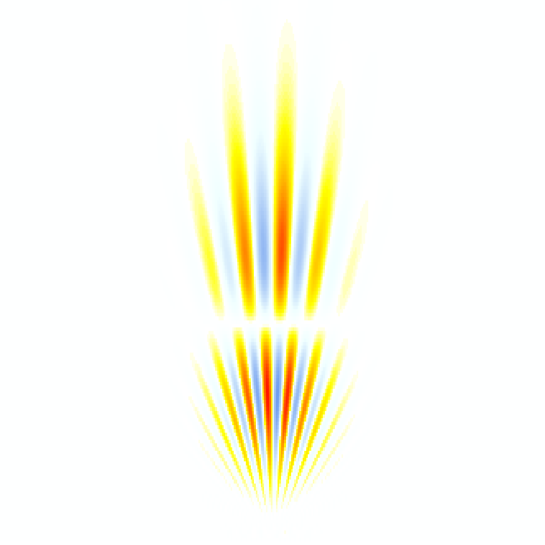
Figure 4.1: Top: Quantum mechanical interference pattern, with averaged trajectories, obtained from a computer simulation employing classical physics only. Bottom: “Entangling current” of Eq. (3.9) for the scenario above.

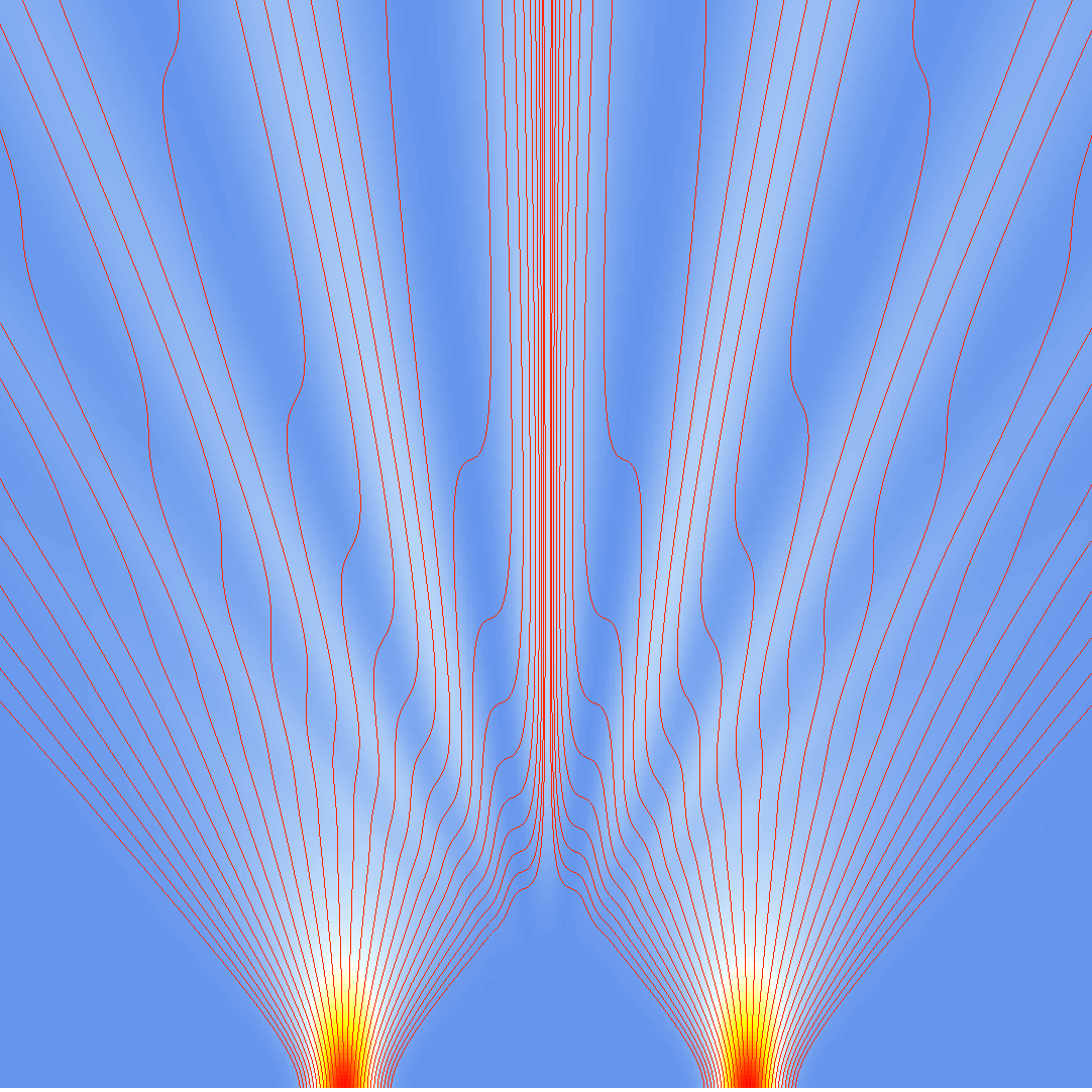
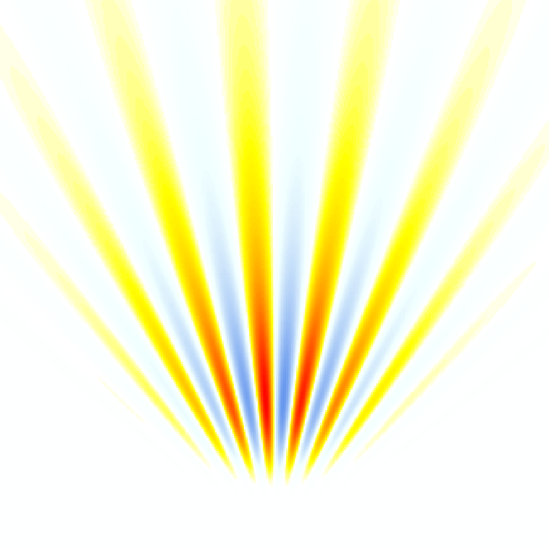
Figure 4.2: Similar scenario as in Fig.4.1, albeit with zero velocity components in the transverse (i.e., $x-$) direction, and with large dispersion instead of a small one. As can be seen from the entangling current in the lower part of the figure, its extrema coincide with the areas where the trajectories’ “kinks” appear, pointing at a rapid crossing-over due to the effects of the diffusive processes involved.

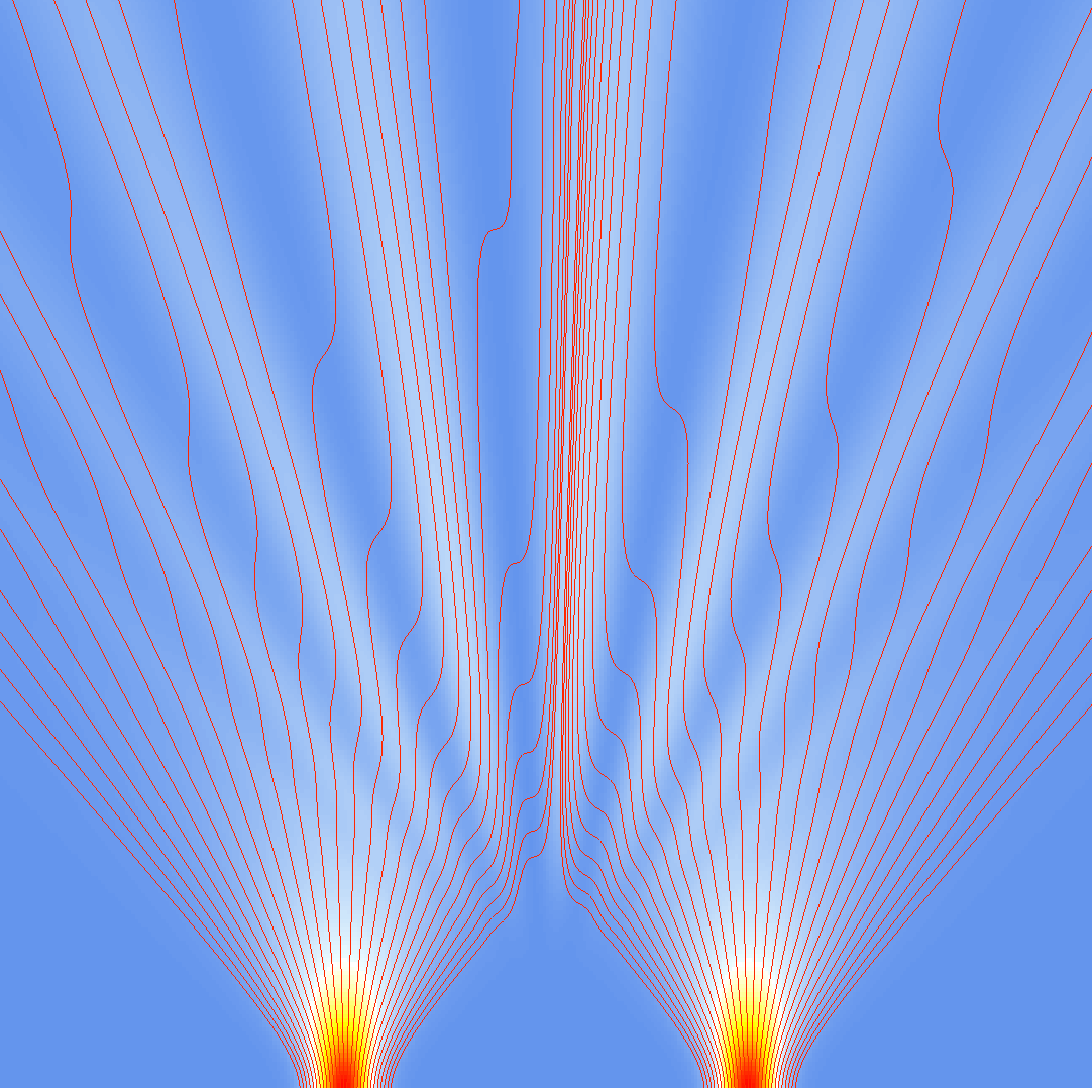
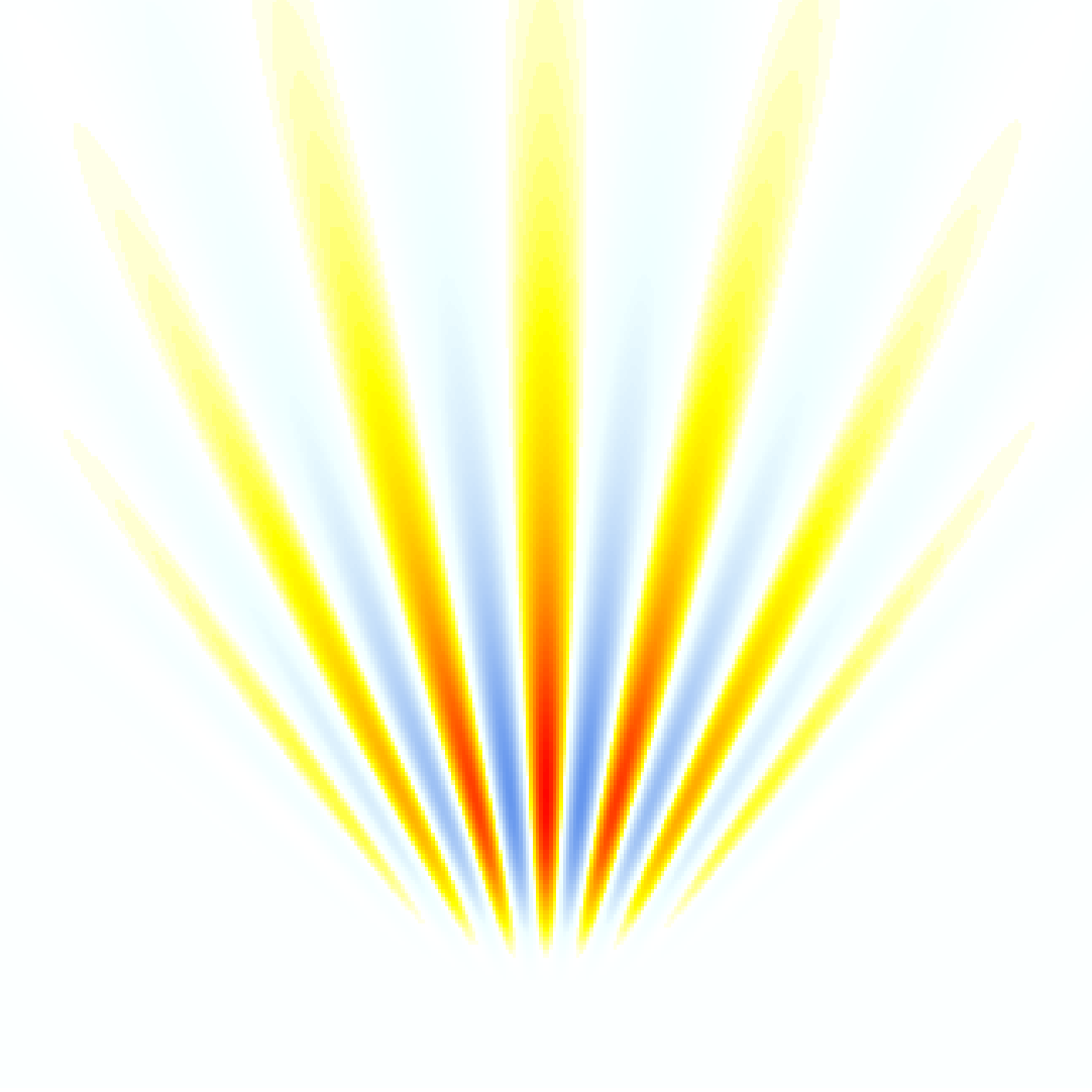
Figure 4.3: Same as Fig.4.2, except that in the left channel a phase shift of $\triangle\varphi=\frac{\pi}{2}$ has been added, thus demonstrating an example of the scalar Aharonov-Bohm effect. Due to the entangling current, or to the diffusion processes, respectively, the intensity maxima of Fig.4.2 are “pushed to the side”, providing the asymmetrical distribution of the interference fringes.

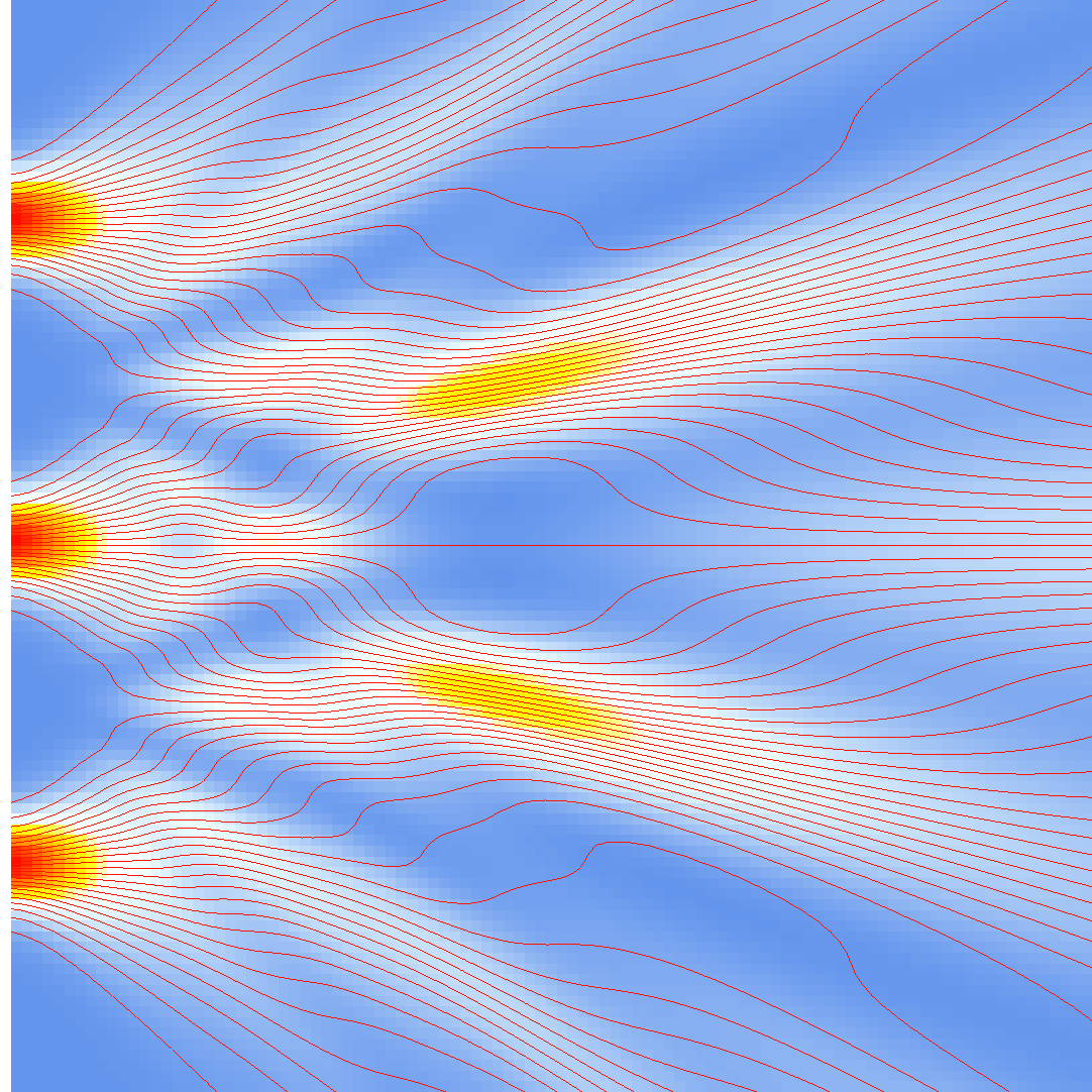
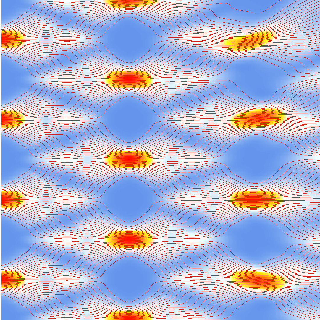
Figure 4.4: Top: A 3-slit system with intensity distributions and averaged trajectories. Bottom: Detail of a system with a large number $n$ of slits (i.e., a so-called Talbot carpet), explicitly showing only four of them. Note that non-spreading “cells” emerge which contain the trajectories and keep them there.

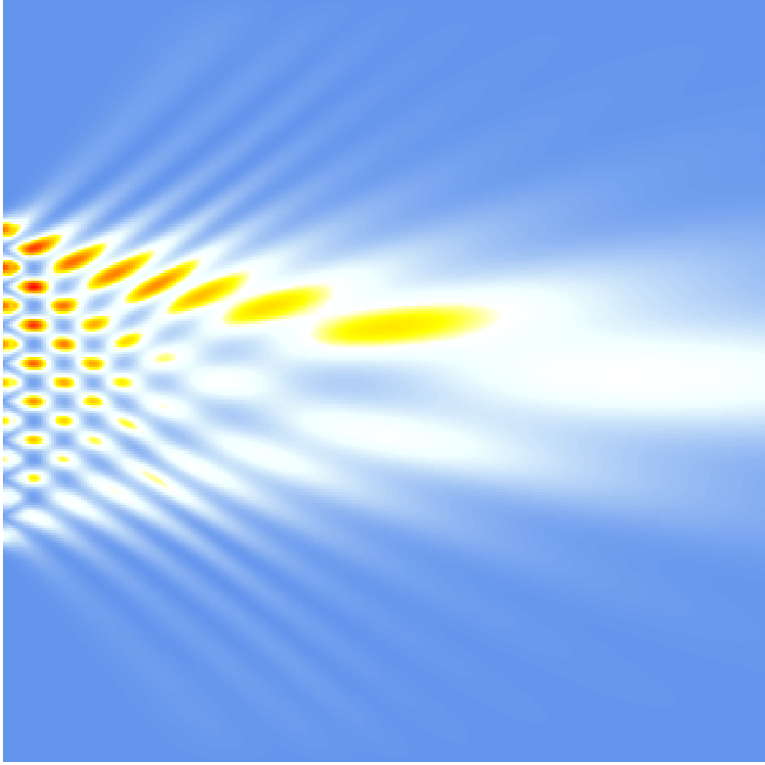
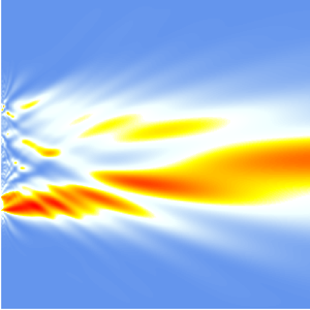
Figure 4.5: Top: Classically simulated interference pattern for a system of 9 slits with gradually diminishing initial intensity distributions. Bottom: Same, except that the initial intensity distributions have been chosen to have random values.

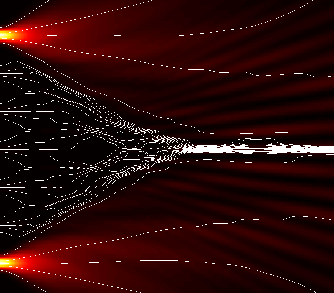
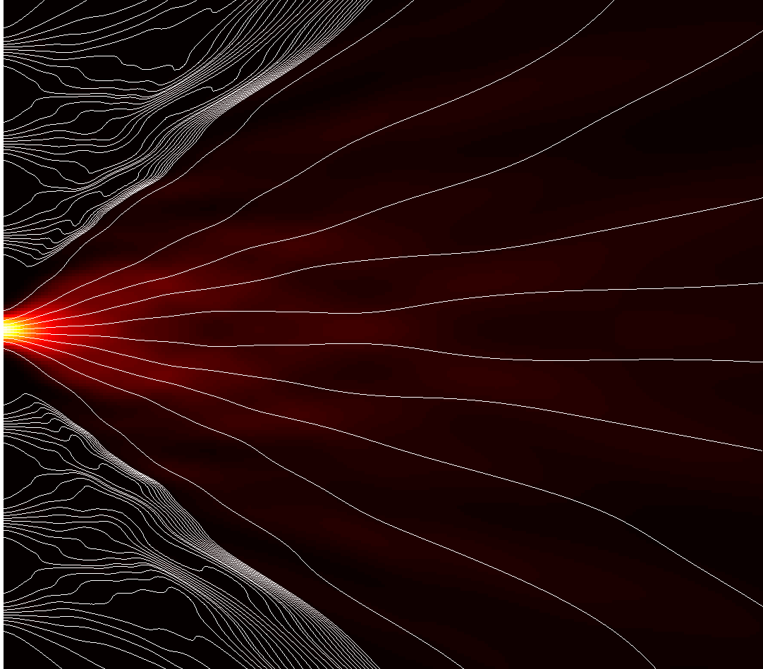
Figure 4.6: Two examples of intensity and trajectory distributions of particularly “weighted” 7-slit systems. Top: Quantum squeezer. Bottom: Quantum sweeper.

References

- (1) Y. Couder, “Yves Couder explains wave/particle duality via silicon droplets [Through the Wormhole].” http://www.youtube.com/watch?v=W9yWv5dqSKk, 2011.
- (2) G. Grössing, “The vacuum fluctuation theorem: Exact schrödinger equation via nonequilibrium thermodynamics,” Phys. Lett. A 372 (2008) 4556–4563, arXiv:0711.4954v2 [quant-ph].
- (3) G. Grössing, “On the thermodynamic origin of the quantum potential,” Physica A 388 (2009) 811–823, arXiv:0808.3539v1 [quant-ph].
- (4) G. Grössing, S. Fussy, J. Mesa Pascasio, and H. Schwabl, “Emergence and collapse of quantum mechanical superposition: Orthogonality of reversible dynamics and irreversible diffusion,” Physica A 389 (2010) 4473–4484, arXiv:1004.4596 [quant-ph].
- (5) G. Grössing, S. Fussy, J. Mesa Pascasio, and H. Schwabl, “Elements of sub-quantum thermodynamics: quantum motion as ballistic diffusion,” J. Phys.: Conf. Ser. 306 (2011) 012046, arXiv:1005.1058 [physics.gen-ph].
- (6) G. Grössing, J. Mesa Pascasio, and H. Schwabl, “A classical explanation of quantization,” Found. Phys. 41 (2011) 1437–1453, arXiv:0812.3561 [quant-ph].
- (7) G. Grössing, S. Fussy, J. Mesa Pascasio, and H. Schwabl, “An explanation of interference effects in the double slit experiment: Classical trajectories plus ballistic diffusion caused by zero-point fluctuations,” Ann. Phys. 327 (2012) 421–437, arXiv:1106.5994 [quant-ph].
- (8) G. Grössing, S. Fussy, J. Mesa Pascasio, and H. Schwabl, “The quantum as an emergent system,” J. Phys.: Conf. Ser. 361 (2012) 012008, arXiv:1205.3393 [quant-ph].
- (9) Y. Couder, S. Protière, E. Fort, and A. Boudaoud, “Dynamical phenomena: Walking and orbiting droplets,” Nature 437 (2005) 208–208.
- (10) Y. Couder and E. Fort, “Single-particle diffraction and interference at a macroscopic scale,” Phys. Rev. Lett. 97 (2006) 154101.
- (11) Y. Couder, A. Boudaoud, S. Protière, and E. Fort, “Walking droplets, a form of wave-particle duality at macroscopic scale?,” Europhys. News 41 (2010) 5.
- (12) Y. Couder and E. Fort, “Probabilities and trajectories in a classical wave-particle duality,” J. Phys.: Conf. Ser. 361 (2012) 012001.
- (13) G. Grössing, ed., Emergent Quantum Mechanics 2011. No. 361/1. IOP Publishing, Bristol, 2012. http://iopscience.iop.org/1742-6596/361/1.
- (14) Y. Aharonov, H. Pendleton, and A. Petersen, “Modular variables in quantum theory,” Int. J. Theor. Phys. 2 (1969) 213–230.
- (15) Y. Aharonov, H. Pendleton, and A. Petersen, “Deterministic quantum interference experiments,” Int. J. Theor. Phys. 3 (1970) 443–448.
- (16) L. V. P. R. de Broglie, Non-Linear Wave Mechanics: A Causal Interpretation. Elsevier, Amsterdam, 1960.
- (17) P. R. Holland, The Quantum Theory of Motion: An account of the de Broglie-Bohm causal interpretation of quantum mechanics. Cambridge University Press, Cambridge, 1993.
- (18) M. J. W. Hall and M. Reginatto, “Schrödinger equation from an exact uncertainty principle,” J. Phys. A: Math. Gen. 35 (2002) 3289–3303.
- (19) E. Fort, A. Eddi, A. Boudaoud, J. Moukhtar, and Y. Couder, “Path-memory induced quantization of classical orbits,” PNAS 107 (2010) 17515–17520.
- (20) A. S. Sanz and S. Miret-Artés, “A trajectory-based understanding of quantum interference,” J. Phys. A: Math. Gen. 41 (2008) 435303, arXiv:0806.2105 [quant-ph].
- (21) G. Grössing, “From classical hamiltonian flow to quantum theory: Derivation of the schrödinger equation,” Found. Phys. Lett. 17 (2004) 343–362, quant-ph/0311109v2.
- (22) J. Tollaksen, Y. Aharonov, A. Casher, T. Kaufherr, and S. Nussinov, “Quantum interference experiments, modular variables and weak measurements,” New J. Phys. 12 (2010) 013023, arXiv:0910.4227v1 [quant-ph].
- (23) J. Mesa Pascasio, S. Fussy, H. Schwabl, and G. Grössing, “Modeling quantum mechanical double slit interference via anomalous diffusion: independently variable slit widths,” Physica A 392 (2013) 2718–2727, arXiv:1304.2885 [quant-ph].
- (24) H. Rauch, “Phase space coupling in interference and EPR experiments,” Phys. Lett. A 173 (1993) 240–242.
- (25) A. Mandelis, Diffusion-wave fields: Mathematical methods and Green functions. Springer, New York, NY, 2001.
- (26) A. Mandelis, L. Nicolaides, and Y. Chen, “Structure and the Reflectionless/Refractionless nature of parabolic diffusion-wave fields,” Phys. Rev. Lett. 87 (2001) 020801.
- (27) G. Grössing, S. Fussy, J. Mesa Pascasio, and H. Schwabl, “”Systemic nonlocality” from changing constraints on sub-quantum kinematics,” J. Phys.: Conf. Ser., In Press (2013) , arXiv:1303.2867 [quant-ph].
- (28) H. R. Schwarz and N. Köckler, Numerische Mathematik. Vieweg+Teubner, 7 ed., 2009.
- (29) A. S. Sanz and S. Miret-Artés, “A causal look into the quantum talbot effect,” J. Chem. Phys. 126 (2007) 234106.