Long-lifetime Polariton BEC in a Microcavity with an Embedded Quantum Well and Graphene

Abstract

We study the propagation of a Bose-Einstein condensate (BEC) of long-lifetime exciton polaritons in a high-quality microcavity with an embedded semiconductor quantum well or a graphene layer using the Gross-Pitaevskii equation. It is shown that in these heterostructures the BEC of the long-lifetime polaritons can propagate over the distance up to 0.5 mm. The obtained results are consistent with the recent experimental observations for GaAs/AlGaAs microcavity. It is demonstrated that the BEC density in a polariton trace in a microcavity with embedded graphene at large distances from the excitation spot is higher for the microcavity with higher dielectric constant. It is also predicted that the propagation of a polariton BEC in a microcavity with graphene is dynamically tunable by changing the gap energy, that makes it potentially useful for applications in integrated optical circuits.

I Introduction

Polaritons are the quantum superposition of photons and excitons in semiconductors or graphene Snoke (2009); Berman et al. (2010); Carusotto and Ciuti (2013). In the past years, formation and spreading of the polariton Bose-Einstein condensate (BEC) in quasi-two-dimensional structures attract attention of experimentalists and theoreticians from the point of view of fundamental physics at nanoscales and due to potential applications of polaritons in integrated circuits for optical and quantum computing High et al. (2008); Liew et al. (2010); Menon et al. (2010). Because the effective mass of the polaritons is much smaller than the atomic masses, the BEC transition temperature is much higher than that for atomic BECs Dalfovo et al. (1999). Another important features of the polariton BEC dynamics is that it is essentially non-equilibrium due to the finite polariton lifetime. The polariton decay is mainly caused by the leakage of photons from an optical microcavity and usually the polariton lifetime is of the order of a few picoseconds, depending on the quality Q-factor of the microcavity Carusotto and Ciuti (2013). It was established that the polariton BEC can move in a planar microcavity in response of the external force or field Sermage et al. (2001); Amo et al. (2009a). However, in “traditional” experiments the characteristic length over which the BEC can spread in the microcavity is limited due to relatively short lifetime of the polaritons Amo et al. (2009a).

The signatures of the polariton BEC were first observed in GaAs-based microcavity Deng et al. (2002a, b, 2007); Balili et al. (2007a, b, 2009) and then in CdTe-based  Kasprzak et al. (2006) and GaN-based microcavities Christopoulos et al. (2070). There are two advantages for observation of a polariton BEC in such heterostructures over a conventional exciton BEC Hanamura and Haug (1977). First, polaritons have an effective mass, which is $\sim 10^{-4}$ times lower than the exciton mass, that results in much higher critical temperature of the BEC transition for polaritons than that for the exciton BEC at the same particle density Snoke (2002); Littlewood (2007); Snoke (2009). Second, the polariton BEC is less sensitive, compared to the exciton BEC, to the disorder caused by unavoidable crystal defects and impurities. It is worth noting that the presence of the defects results in the exciton localization in a fluctuating potential in a sample and can destroy an exciton BEC Szymanska and Littlewood (2002); Marchetti et al. (2004, 2006); Malpuech et al. (2007).

It was found Saba et al. (2001); Deng et al. (2002a, b); Kasprzak et al. (2006); Deng et al. (2007); Lagoudakis et al. (2008); Utsunomiya et al. (2008); Nelsen et al. (2009); Balili et al. (2009); Roumpos et al. (2012) that for optimal conditions of the polariton BEC formation the quality Q-factor of the optical microcavity should be enough high. The increase of the microcavity Q-factor leads to the increase of the polariton densities in the microcavity and, also, to longer polariton lifetime thus presenting more favorable conditions for the BEC observations. Also, enough strong exciton-photon coupling (Rabi splitting) is needed thus, requiring large quantum well (QW) exciton oscillator strength. Enough large polariton-polariton interaction scattering cross-section is also an important factor, which provides efficient thermalization in the polariton system and hence short enough relaxation time for the transition of the system to a BEC (see Ref. Snoke (2002) for the discussion). Rapid expansion of a spatial coherence and the polariton BEC formation dynamics in a GaAs-based microcavity has been recently observed in Ref. Belykh et al. (2013).

In the present Article we consider the dynamics of polaritons formed by the cavity photons and the excitons in GaAs a quantum well and graphene embedded in a microcavity. Our studies are motivated by experiments Sermage et al. (2001) and Nelsen et al. (2012) where the directional propagation of exciton polaritons have been observed in the presence of an external force. In particular, in Ref.  Nelsen et al. (2012) the possibility of synthesis of a semiconductor microcavity with the Q-factor exceeding $10^{5}$ has been demonstrated for the first time. That allowed one to observe the polaritons with extremely long lifetime $\sim 100$ ps, that is $\sim 30\times$ longer than that in the traditional experiments Carusotto and Ciuti (2013). It was found Nelsen et al. (2012) that the long-lifetime polaritons in a planar microcavity could propagate over a macroscopic scale of a fraction of millimeter order. It was supposed in Ref. Nelsen et al. (2012) that a BEC coherent flow formed at high enough densities of the long-lifetime polaritons have promoted their long-distance propagation. In this Article, we demonstrate that the polariton dynamics observed in Ref. Nelsen et al. (2012) is consistent with that predicted from the Gross-Pitaevskii equation for a polariton BEC. Specifically, we show that under the action of an external force, a long-lifetime polariton BEC can propagate over the distance $\sim 0.5$ mm from the excitation spot. It is demonstrated that the polariton-exciton interactions can also significantly change the spatial distribution of the polaritons in the BEC. Based on the obtained results, we propose an observation of long-lifetime polariton BEC formed in a graphene layer embedded into a high-Q microcavity. It is shown that for graphene there is an additional controlling parameter – the energy gap in the electron and hole excitation spectra – that allows one to govern the polariton BEC propagation. The possibility to dynamically adjust the properties of the polariton BEC by changing the gap, for example through application of the electric field, makes a microcavity with embedded graphene a promising candidate for the use in adaptive optical circuits.

Our article is organized in the following way. In Sec. II the dynamics of a Bose-Einstein condensate of long-lifetime exciton polaritons in a microcavity with an embedded semiconductor quantum well or a grapheme layer is considered based on the Gross-Pitaevskii equation. The details of the numerical simulations are presented in Sec. III. Sec. IV presents the results of the simulations of the polarition BEC propagation in a microcavity with an embedded quantum well and an embedded graphene layer. Here, the effect of the polariton lifetime on the BEC dynamics is discussed and the comparison of the BEC propagation in a microcavity with an embedded quantum well and graphene is presented. Finally, the conclusions follow in Sec V.

II Dynamics of an exciton-polariton BEC in a microcavity

At temperature much lower than the BEC transition temperature the dynamics of the exciton polariton BEC is described by the Gross-Pitaevskii equation

$$i\hbar\frac{\partial\Psi(\bm{r},t)}{\partial t}=-\frac{\hbar^{2}}{2m}\Delta\Psi(\bm{r},t)+U(\bm{r})\Psi(\bm{r},t)$$

$$\,\,\,\,\,\,+g\Psi(\bm{r},t)|\Psi(\bm{r},t)|^{2}-i\hbar\gamma\Psi(\bm{r},t)+i\hbar G(\bm{r}).$$ (1)

In Eq. (1) $\Psi(\bm{r},t)$ is the condensate wave function which depends on the coordinates $\bm{r}=(x,y)$ in the plane of the microcavity and time $t$, $m$ is the polariton mass, $g$ is the effective interaction strength proportional to the polariton-polariton scattering amplitude, $\gamma=1/2\tau$ is the decay rate, $\tau$ is the polariton lifetime, and $G(\bm{r})$ is the source term. The term $U(\bm{r})=U_{\rm ex-pol}(\bm{r})+U_{\rm ext}(\bm{r})$ describes the repulsive interaction $U_{\rm ex-pol}(\bm{r})$ of the polaritons with those excitons in a quantum well, which are not coupled with the microcavity photons, and the potential energy due to the external force, $U_{\rm ext}(\bm{r})$. Importance of the interactions of polaritons with the exciton cloud has been recently discussed in Ref. Christmann et al. (2012). The corresponding interaction energy is

$$U_{\rm ex-pol}(\bm{r})=X_{0}^{2}g_{\rm ex-ex}n_{\rm ex}(\bm{r}),$$ (2)

where $X_{0}\equiv X_{\bm{k}=0}$ is the Hopfield coefficient for the exciton component in the polariton wave function taken at the wave vector $\bm{k}=0$, $g_{\rm ex-ex}$ is the exciton-exciton repulsive interaction constant and $n_{\rm ex}(\bm{r})$ is the exciton density in the cloud. The Hopfield coefficient for arbitrary wave-vector $k$ is

$$X_{k}=\frac{1}{\sqrt{1+\left({\hbar\Omega_{R}\over E_{\rm LP}(k)-E_{\rm C}(k)}\right)^{2}}},$$ (3)

where $\Omega_{R}$ is the Rabi splitting,

$$E_{\rm LP}(k) = {E_{\rm C}(k)+E_{\rm X}(k)\over 2}$$ (4)

$$-{1\over 2}\sqrt{(E_{\rm C}(k)-E_{\rm X}(k))^{2}+4(\hbar\Omega_{R})^{2}}$$

is the energy of the lower polariton branch, $E_{\rm X}(k)$ is the exciton energy and $E_{\rm C}(k)$ is the cavity photon energy as functions of $k$ Ciuti et al. (2003). Because the polaritons in the BEC are condensed into the state with small wave-vectors $\bm{k}$, the Hopfield coefficient in Eq. (2) is taken at $\bm{k}=0$. We approximate the exciton density in the cloud via a Gaussian profile as $n_{\rm ex}(\bm{r})=n_{0}\exp(-|\bm{r}-\bm{r_{0}}|^{2}/a^{2})$ where $n_{0}$ is the density at the center of the cloud and $a$ is the characteristic size of the cloud. The Gaussian profile gives the required bell-like dependence for the exciton cloud density in the excitation area $|\bm{r}-\bm{r_{0}}|\sim a$ and also captures the sharp drop of the exciton density at large distances $|\bm{r}-\bm{r_{0}}|\gg a$ Dalfovo et al. (1999). Thus, the polariton-exciton interaction (2) is represented as

$$U_{\rm ex-pol}(\bm{r})=U_{0}\exp(-|\bm{r}-\bm{r_{0}}|^{2}/a^{2}),$$ (5)

where $U_{0}=X_{0}^{2}g_{\rm ex-ex}n_{0}$. To study the effects of the polariton-exciton cloud interaction, we vary the interaction strength $U_{0}$ as described below.

It has been demonstrated in recent experiments Sermage et al. (2001); Nelsen et al. (2012) that the microcavity polaritons can be accelerated by an external force due to the spatial gradient of thickness of the microcavity. In this approach, the average force acting upon a polariton wave packet at the point $\bm{r}$ is $\bm{F}(\bm{r})=-\nabla E_{\rm C}(\bm{r})$, where $E_{\rm C}(\bm{r})$ is energy of the polariton band taken at the in-plane vector of the polariton $\bm{k}=0$ Sermage et al. (2001). In particular, in experiments Sermage et al. (2001); Nelsen et al. (2012) the microcavity width, and hence the energy $E_{C}(\bm{r})$, has been a linear function a spatial coordinate (the wedge-shape geometry of the microcavity) that resulted in a constant force $\bm{F}(\bm{r})=\bm{F}_{0}$ acting upon the polaritons. To describe the effect of the force, we set the corresponding potential energy as

$$U_{\rm ext}(\bm{r})=-F_{0}x.$$ (6)

To explore the polariton BEC dynamics in a macroscopically large sample we consider the case where the source of polaritons, $G(\bm{r})$, is localized in space Roumpos et al. (2012). Within the used approximation, the source term is represented as $G(\bm{r})=G_{0}\exp(-|\bm{r}-\bm{r_{0}}|^{2}/a^{2})$ with the same characteristic size $a$ as for the exciton cloud size.

Following the conditions of the experiments Sermage et al. (2001); Nelsen et al. (2012), we varied $U_{0}$ from 0 to 10 meV and $F_{0}$ from 0 to 13 meV/mm. For the long-lifetime polaritons in a microcavity with the quality factor $Q\sim 10^{6}$ with an embedded semiconductor QW we set $\tau=100$ ps Nelsen et al. (2012), $m=10^{-4}m_{0}$ where $m_{0}$ is the free electron mass Carusotto and Ciuti (2013), and $g=10^{-2}$ meV$\mu$m² Amo et al. (2009a).

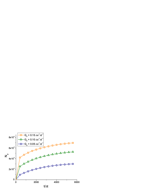
Figure 1: Time dependence of the total number of polaritons in the BEC for $F_{0}=13$ meV/mm and $U_{0}=3$ meV for different pumping rates $G_{0}$.

Formation of the polariton BEC in gapped graphene has recently been predicted in Ref. Berman et al. (2012a). The polariton effective mass in graphene is

$$m=2(m_{\rm ex}^{-1}+cL_{c}/\sqrt{\varepsilon}\pi\hbar)^{-1},$$ (7)

where $m_{\rm ex}$ is the exciton effective mass in graphene, $L_{c}$ is the length of the microcavity, $\varepsilon$ is the dielectric constant of the microcavity, and $c$ is the speed of light in vacuum. In the present work we consider the case of zero detuning where the cavity photons and the excitons in graphene are in resonance at $\bm{k}=0$. In this case the length of the microcavity is chosen as Berman et al. (2012b)

$$L_{c}=\frac{\hbar\pi c}{(2\delta-V_{0}+C/\delta^{2})\sqrt{\varepsilon}},$$ (8)

where $V_{0}=e^{2}/4\pi\varepsilon\varepsilon_{0}r^{\prime}$, $C=(\hbar ev_{F})^{2}/8\pi\varepsilon\varepsilon_{0}r^{\prime 3}$, $\delta$ is the gap energy in the quasiparticle spectrum, and $v_{F}$ is the Fermi-velocity of the electrons in graphene. The parameter $r^{\prime}$ is found from the following equation,

$$2\delta^{2}(2\delta-\hbar\omega)r^{\prime 3}-2D\delta^{2}r^{\prime 2}+D(\hbar v_{F})^{2}=0,$$ (9)

where $D=e^{2}/4\pi\varepsilon\varepsilon_{0}$. For dipolar excitons in GaAs/AlGaAs coupled quantum wells, the energy of the recombination peak is $\hbar\omega=1.61$ eV Negoita et al. (1999). We expect similar photon energies in graphene. However, its exact value depends on the graphene dielectric environment and substrate properties though. The exciton effective mass in Eq. (7) is given by

$$m_{\rm ex}=\frac{2\delta^{4}}{Cv_{F}^{2}}.$$ (10)

The polariton-polariton interaction strength is Berman et al. (2012a); Ciuti et al. (2003)

$$g={3e^{2}a_{B}\over 8\pi\varepsilon_{0}\varepsilon},$$ (11)

where $a_{B}=2\pi\varepsilon_{0}\varepsilon\hbar^{2}/m_{r}e^{2}$ is the two-dimensional Bohr radius of the exciton, $m_{r}$ is the exciton reduced mass.

Formation of the excitons in graphene requires a gap in the electron and hole excitation spectra, which can be created, for example, by external electric field Kuzmenko et al. (2009); Mak et al. (2009); Zhang et al. (2009). We do not restrict our consideration to a specific mechanism of the gap formation. As follows from Eqs. (7)–(11), both the polariton mass $m$ and the interaction strength $g$ in gapped graphene depend on the gap energy $\delta$. In our studies, we varied $\delta$ from 0.1 eV to 0.5 eV that are the representative values for graphene. The polariton lifetime is mainly defined by the leakage of the photons through the mirrors and only weakly depends on the exciton lifetime Carusotto and Ciuti (2013); Nelsen et al. (2012). Therefore, we use the same polariton lifetime $\tau=100$ ps for graphene and for a semiconductor quantum well.

III Numerical simulations

To study the polariton BEC dynamics, we numerically integrated Eq. (1). At the initial moment $t=0$ we set $\Psi(\bm{r},0)=0$. As is demonstrated in Sec. IV below, the long-lifetime polaritons accelerated by the external force can propagate over distances up to $l_{\rm max}\sim 0.5$ mm from the excitation spot. The characteristic wavelength of the polariton wave packet at the distance $l\approx l_{\rm max}$ can be estimated quasiclassically as $\lambda_{\rm min}\approx 2\pi\hbar/\sqrt{2m(F_{0}l_{\rm max}+U_{0})}$ that gives $\lambda_{\rm min}\approx 9.5\times 10^{-7}$m for $F_{0}=13$ meV/mm and $U_{0}=10$ meV. At shorter distances $l<l_{\rm max}$ one has $\lambda>\lambda_{\rm min}$. To resolve the oscillations of the polariton wavefunction with the wavelengths $\lambda\geq\lambda_{\rm min}$, we choose the numerical grid spacing $\Delta x=1.5\times 10^{-7}$ m. The dimensions of the numerical box are $L_{x}\times L_{y}=6000\times 3000\,(\Delta x)^{2}$. The long side of the numerical box is arranged parallel to the direction of the constant force $\bm{F}_{0}$. We use the periodical boundary conditions at the numerical box boundaries. The unit of time is equal to $\Delta t=2m(\Delta x)^{2}/\hbar=3.9\times 10^{-14}$ s. We numerically integrated Eq. (1) over time with the 4^th order Runge-Kutta scheme at the time step $h=10^{-2}\Delta t$. An explicit 4^th order accuracy method has been used to represent the Laplacian operator in Eq. (1). We took advantage of the graphical processing unit CUDA programming Nvi that allowed us to achieve $\sim 20\times$ increase of the performance with respect to the shared-memory parallel version of the code. This allowed us to perform the simulations for this macroscopic system within practically realizable time intervals. The overall computation time for a single run was $\sim 10$ hours on NVIDIA Tesla S2050 card.

IV Propagation of a BEC of long-lifetime polartions in a microcavity

IV.1 Polartion BEC in a microcavity with an embedded quantum well

In this Section we focus on the propagation of a BEC of long-lifetime polaritons in a microcavity with an embedded semiconductor QW. Fig. 1 shows the time dependence of the total number of polaritons $N_{p}(t)=\int d^{2}\bm{r}|\Psi(\bm{r},t)|^{2}$ after the source it turned on. It follows from Fig. 1 that after the system approaches a steady state at $t\sim 6\times 10^{3}\Delta t\approx 230$ ps, for the pumping rate $G_{0}=0.1\Delta x^{-1}\Delta t^{-1}$ the total number of polaritons is $N_{p}\sim 5.3\times 10^{4}$ that is a representative value for experiments with exciton polaritons in a semiconductor microcavity Nelsen et al. (2012). Below we used this pumping rate in our simulations.

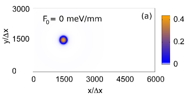
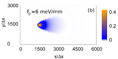
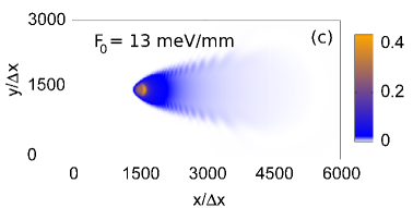
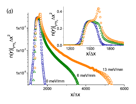
Figure 2: (a-c) Evolution of a trace of the long-lifetime polariton BEC with increasing the force $F_{0}$ for $t=4800\Delta t$ and $U_{0}=3$ meV. The colorbars show the dimensionless BEC density $n(\bm{r})\Delta x^{2}$. (d) Evolution of a steady-state polariton density at $y=y_{0}$ for $U_{0}=3$ meV with increasing $F_{0}$ shown in a logarithmic scale and in a linear scale in the region around the excitation spot (inset).

Propagation of long-lifetime polariton BEC in the quantum well plane is shown in Fig. 2. The center of the excitation spot is positioned at $\bm{r}_{0}=(x_{0},y_{0})$ where $x_{0}=y_{0}=1500\Delta x$. The evolution of the long-lifetime polariton BEC distribution with increasing of the force $F_{0}$ is given in Fig. 2a-c. Fig. 2a shows that in the absence of the force the polariton spot is symmetric in the $(x,y)$ plane and has a characteristic size of $\approx 500\Delta x=75$ $\mu$m that is, $\sim 7.5\,a$. With the increase of the force a polariton “trace” is formed and at $F_{0}=13$ meV/mm the length of the trace reaches $\sim 3.5\times 10^{3}\Delta x\approx 500$ $\mu$m (Fig. 2c). To characterize the steady-state polariton distribution in details we plot in Fig. 2d the polariton BEC density at $y=y_{0}$ that is, a cross-section of Fig. 2a-c along the line passing through the center of the excitation spot. The inset in Fig. 2d shows that for the force $F_{0}=13$ meV/mm, the maximum of the polariton density is shifted from the center of the excitation spot $x_{0}$ to $x\approx 1620\Delta x$.

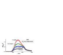
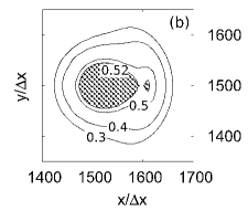
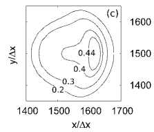
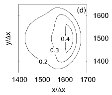
Figure 3: (a) Changes in the polariton density at $y=y_{0}$ with the increase of $U_{0}$ from 1 meV to 3 meV for $t=5.8\times 10^{3}\Delta t$. (b-d): Contour plots for the polariton density for $U_{0}=$ 2 (b), 2.5 (c), and 3 meV (d); other parameters are the same as in plot (a). The contour lines are labeled with the values of the density $n(\bm{r})\Delta x^{2}$. In plot (b) the area with $n(\bm{r})\Delta x^{2}\geq 0.52$ is gray-shaded.

To prove that the shift of the density maximum is caused by the interaction of the polaritons with the exciton cloud, we investigated evolution of the polariton density with changes of the maximum effective interaction strength $U_{0}$. Fig. 3a demonstrates changes in the dimensionless polariton density along the line $y=y_{0}$ with the rise of $U_{0}$ from 1 meV through 3 meV. It is seen that the position of the maximum of the density is shifted from $x\approx 1500\Delta x$ at $U_{0}=1$ meV to $x\approx 1620\Delta x$ at $U_{0}=3$ meV. Fig. 3b-d shows the contour lines for the polariton density $n(\bm{r})$ for different $U_{0}$. From Fig. 3b it is evident that at $U_{0}=2$ meV and $y=y_{0}=1500\Delta x$ the spatial polariton distribution has two maxima positioned at $x\approx 1500\Delta x$ and $1620\Delta x$. While increasing $U_{0}$ to 2.5 meV the left maximum disappears and the right maximum becomes more pronounced, as seen in Fig. 3c. With the further increase of $U_{0}$, most polaritons are concentrated around the maximum at $x\approx 1620\Delta x$ (Fig. 3d).

To clarify the reasons for the shift of the density maximum while $U_{0}$ is increased, we compare in Fig. 4 the distribution of the polariton flux in a steady state $\bm{j}(\bm{r})=({\hbar/2im})\left(\Psi^{*}(\bm{r})\nabla\Psi(\bm{r})-\Psi(\bm{r})\nabla\Psi^{*}(\bm{r})\right)$ for different forces. For $F_{0}=0$ the flux $\bm{j}(\bm{r})$ is distributed symmetrically around the center of the excitation spot. As is seen in Fig. 4a the magnitude of the flux, $j$, reaches its maximum at the distance $\sim 120\Delta x$ from the excitation spot center $\bm{r}_{0}$. The presence of the maximum of $j$ at certain distance from the point $\bm{r}_{0}$ can be understood if one considers the creation and propagation of polariton wave packets in the potential energy profile $U_{\rm ex-pol}(\bm{r})$. The polaritons are accelerated due to the force $\bm{F}_{\rm ex-pol}(\bm{r})=-\nabla U_{\rm ex-pol}(\bm{r})$ and hence, their velocity $v$ gradually rises with the distance from the center. At large distances, the velocity $v$ tends to a constant because the force $\bm{F}_{\rm ex-pol}(\bm{r})$ vanishes. On the other hand, the polariton density $n(\bm{r})$ falls at large distances from $\bm{r}_{0}$ due to spreading of the polaritons over the sample. In effect, the flux $j=nv$ reaches the maximum at certain distance $\sim a$ from the excitation spot center.

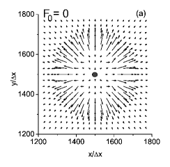
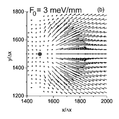
Figure 4: Polariton flux $\bm{j}$ for $U_{0}=3$ meV, $t=5.6\times 10^{3}\Delta t$. The length of the arrows is proportional to the magnitude of the flux $|\bm{j}|$. The point at $\bm{r}_{0}=(1500\Delta x,1500\Delta x)$ marks the center of the pumping spot.

In the presence of a force $\bm{F}_{0}$, the polariton flux distribution acquires a strongly asymmetric form. The result of the simulations for $F_{0}=3$ meV/mm and $U_{0}=3$ meV is shown in Fig. 4b. The simulations for other forces $F_{0}$ and energies $U_{0}$ resulted in the polariton flux distributions, which were similar to that shown in Fig. 4b. In this case, most of the polaritons move in the direction of the force $\bm{F}_{0}$. This results in the shift of the maximum of the polariton density from the spot center, in agreement with Fig. 1d and Fig. 3. It is worth noting that at distances $\sim a$ from the excitation spot center there is a finite flux directed opposite to the external force $\bm{F}_{0}$. However, these polaritons eventually flow around the excitation spot and, at large distances from the spot, move in the direction of the force in agreement with the observations in Ref. Nelsen et al. (2012).

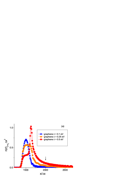
Figure 5: (a) Variation of the density of a long-lifetime polariton BEC in a microcavity with embedded graphene with rising the gap energy $\delta$. (b) Points: dependence of the polariton BEC density at the point $\bm{r}=(2000\Delta x,1500\Delta x)$ (marked by a vertical arrow in plot (a)) with changing $\delta$. Vertical errorbars show uncertainty due to small time-dependent oscillations of the polariton density about the mean values. The dashed curve is a guide to the eye. $F_{0}=13$ meV/mm and $U_{0}=5$ meV for both plots (a) and (b).

IV.2 Polariton BEC dynamics in a microcavity with embedded graphene

Within the same approach, we also studied the propagation of polaritons in a semiconductor microcavity with gapped graphene embedded into it. First, we consider the case of the GaAs-based microcavity, for which we set $\varepsilon=13$. The effective mass $m$ of the polaritons and the polariton-polariton interaction strength $g$ have been found from Eqs. (7)–(11) for different values of the gap energy $\delta$. The results of the simulations for graphene in Fig. 5a shows that the polariton density in the trace gradually increases with rising the gap energy. To characterize the increase of the polariton BEC density in the trace with changing the gap energy we present in Fig. 5b the dependence of the dimensionless polariton density at the point $\bm{r}_{1}=(2000\Delta x,1500\Delta x)$ on the gap energy $\delta$. The point $\bm{r}_{1}$ is positioned at the distance of $500\Delta x\approx 75$ $\mu$m from the excitation spot center $\bm{r}_{0}$. The position of the point $\bm{r}_{1}$ is marked by a vertical arrow in Fig. 5a. Fig. 5b shows that the polariton density at the point $\bm{r}_{1}$ increases in $10.2\times$, from $n\approx 0.013\Delta x^{-2}$ to $n\approx 0.133\Delta x^{-2}$, with changing $\delta$ from 0.1 eV to 0.5 eV. Additionally, the shift of the density maximum in the direction of the external force $\bm{F}_{0}$ is more pronounced for larger $\delta$, as shown in Fig. 5a.

Figure 6: Dependence of the polariton BEC density in a microcavity with embedded graphene at the point $\bm{r}_{1}=(2000\Delta x,1500\Delta x)$ on the microcavity dielectric constant $\varepsilon$. The dashed line is a guide to the eye.

The microcavity can be synthesized from different semiconductor materials. To study the effect of the microcavity material we investigated the propagation of the long-lifetime polariton BEC in graphene in microcavities formed by semiconductor materials CuBr, ZnSe, CdTe, and ZnO Berger (1997) that is, by those materials, which were utilized for the experimental studies of microcavity polaritons Kelkar et al. (1997); Dang et al. (1998); Saba et al. (2001); Zamfirescu et al. (2002); Kasprzak et al. (2006); Christopoulos et al. (2070); Manni et al. (2011); Kawase et al. (2012); Nakayama et al. (2012). According to Eqs. (7)–(11), changes in the dielectric constant $\varepsilon$ of the microcavity result in the variations of the microcavity length $L_{c}$, for which the cavity photons and excitons in graphene are in the resonance, as well as in the changes in the polariton effective mass $m$ and the polariton interaction strength $g$. It was found that the BEC density distributions for CuBr ($\varepsilon=5.7$), ZnSe ($\varepsilon=9.1$), CdTe ($\varepsilon=10.2$) and ZnO ($\varepsilon=10.8$) microcavities are qualitatively similar to those obtained for the microcavity synthesized from GaAs and considered above in this Section. To characterize the details of the changes in the polariton BEC distribution in those microcavities, we plot in Fig. 6 the dependence of the dimensionless density of the condensate, $n(\bm{r})\Delta x^{2}$, at the point $\bm{r}_{1}=(2000\Delta x,1500\Delta x)$, similarly to that shown in Fig. 5 for a GaAs-based microcavity. It is seen in Fig. 6 that the polariton density at the distance $\sim 75$ $\mu$m from the excitation spot center gradually decreases with the decrease of the dielectric constant of the microcavity material. However, this variation is slow: the change of the dielectric constant from $\varepsilon=13$ (GaAs) to 5.7 (CuBr) only results in $\sim 19$% decrease of the BEC density from $n\approx 0.133\Delta x^{-2}$ to $n\approx 0.108\Delta x^{-2}$. Thus, the BEC density in a polariton trace in a microcavity with embedded graphene at large distances from the excitation spot is higher for the microcavity with high dielectric constant.

In Ref. Berman et al. (2012a) it was shown that the Kosterlitz-Thouless transition temperature $T_{c}$ for polaritons in a microcavity with embedded graphene increases with the decrease of the microcavity dielectric constant $\varepsilon$. On the other hand, from the consideration above it follows that the increase of $\varepsilon$ leads to higher BEC densities at a large distance from the excitation spot. These conclusions are consistent with each other because Ref. Berman et al. (2012a) describes the redistribution of the polaritons in the superfluid between the normal and superfluid components at finite temperature, whereas in the present work we consider the dynamics of the system at a given total number of the polaritons in the BEC in the low temperature limit $T\ll T_{c}$.

IV.3 Effect of the polariton lifetime on the BEC dynamics

Finally, to demonstrate the effect of the polariton lifetime on the BEC dynamics, we studied the BEC spreading in a semiconductor quantum well in a microcavity for traditional, short-lifetime polaritons, for which we took $\tau=3$ ps Amo et al. (2009a). In Fig. 7 we compare the BEC density for the short-lifetime polaritons in a microcavity with GaAs QW with that for the long-lifetime polaritons in a microcavity with GaAs QW and with embedded graphene at $\delta=0.5$ eV. It is clearly seen that for the short-lifetime polaritons, even in the presence of an external force, the BEC is mostly located in the region where it is directly excited by the external pumping and its density rapidly decreases at large distances from the excitation spot. Fig. 7 also shows that the long-lifetime polariton BEC density in graphene with $\delta=0.5$ eV is higher than that in the GaAs quantum well in a microcavity at large distances from the excitation spot.

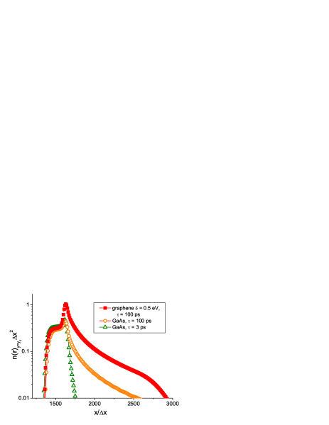
Figure 7: Density of a long-lifetime polariton BEC in graphene for $U_{0}=5$ meV and $\delta=0.5$ eV, in a GaAs-based microcavity for $U_{0}=3$ meV, and of short-lifetime polariton BEC in a GaAs-based microcavity with $\tau=3$ ps for $U_{0}=5$ meV. The force is $F_{0}=13$ meV/mm.

IV.4 Comparison of the BEC propagation in microcavity with an embedded quantum well and graphene

From the results obtained in Sec. IV.1 – IV.3 it follows that the propagation dynamics of the long-lifetime polariton BEC in a microcavity with an embedded GaAs quantum well and in a microcavity formed by GaAs, ZnSe, CdTe, and CuBr with an embedded graphene layer are quantitatively similar to each other. However, the polariton BEC density in the trace for a GaAs-based microcavity with embedded graphene at $\delta=0.5$ eV is higher than that for a microcavity with GaAs QW, as is demonstrated in Fig. 7. The BEC density in the microcavity with embedded graphene sharply increases with the rise of the gap energy $\delta$, as shown in Fig. 5b. This allows one to utilize the gap energy in graphene as a parameter that controls the polariton BEC propagation in a microcavity. The polariton BEC density far from the excitation spot gradually decreases with the decrease of the dielectric constant of the microcavity material, thus semiconductors with higher dielectric constant provide better conditions for the observation of the polariton BEC propagation.

V Conclusion

Through simulations of the exciton polariton BEC dynamics by using the non equilibrium Gross-Pitaevskii equation, we demonstrated that the long-lifetime ($\tau\sim 100$ ps) polaritons in a wedge-shaped microcavity can propagate over a macroscopically long distance $\sim 500$ $\mu$m. This distance is large compared to that for short-lifetime polaritons in traditional experiments Snoke (2002); Kasprzak et al. (2006); Amo et al. (2009b, a); Sermage et al. (2001). The maximum of the polariton density in the BEC is shifted from the center of the excitation spot in the direction of the external force due to the exciton-polariton interaction.

We also proposed to observe a polariton BEC propagation in a microcavity with an embedded gapped graphene layer. It was found that the BEC density at large distances from the excitation spot in a semiconductor quantum well and in gapped graphene are comparable with each other. However, in graphene there is an additional parameter that controls the long-lifetime polariton propagation, which is the energy of a gap in the electron and hole energetic spectra. The obtained results can be useful for practical applications of coherent polariton flow in a high-quality microcavity in working elements of integrated optical circuits High et al. (2008); Liew et al. (2010); Menon et al. (2010). The advantage of graphene in a microcavity is that the propagation of a polariton BEC is dynamically tunable via electrostatic gating.

References

- Snoke (2009) D. W. Snoke, Solid State Physics: Essential Concepts (Addison-Wesley, San Francisco, 2009).
- Berman et al. (2010) O. L. Berman, R. Y. Kezerashvili, Y. E. Lozovik, and D. W. Snoke, Phil. Trans. R. Soc. A 368, 5459 (2010).
- Carusotto and Ciuti (2013) I. Carusotto and C. Ciuti, Rev. Mod. Phys. 85, 299 (2013).
- High et al. (2008) A. A. High, E. E. Novitskaya, L. V. Butov, M. Hanson, and A. C. Gossard, Science 321, 229 (2008).
- Liew et al. (2010) T. C. H. Liew, A. V. Kavokin, T. Ostatnicky, M. Kaliteevski, I. A. Shelykh, and R. A. Abram, Phys. Rev. B 82, 033302 (2010).
- Menon et al. (2010) V. M. Menon, L. I. Deych, and A. A. Lisyansky, Nature Photonics 4, 345 (2010).
- Dalfovo et al. (1999) F. Dalfovo, S. Giorgini, L. P. Pitaevskii, and S. Stringari, Rev. Mod. Phys. 71, 463 (1999).
- Sermage et al. (2001) B. Sermage, G. Malpuech, A. V. Kavokin, and V. Thierry-Mieg, Phys. Rev. B 64, 081303(R) (2001).
- Amo et al. (2009a) A. Amo, J. Lefrere, S. Pigeon, C. Adrados, C. Ciuti, I. Carusotto, R. Houdre, E. Giacobino, and A. Bramati, Nat. Physics 5, 805 (2009a).
- Deng et al. (2002a) H. Deng, G. Weihs, C. Santori, J. Bloch, and Y. Yamamoto, Science 298, 199 (2002a).
- Deng et al. (2002b) H. Deng, G. Weihs, D. Snoke, J. Bloch, and Y. Yamamoto, PNAS 100, 15318 (2002b).
- Deng et al. (2007) H. Deng, G. Solomon, R. Hey, K. Ploog, and Y. Yamamoto, Phys. Rev. Lett. 99, 126403 (2007).
- Balili et al. (2007a) R. Balili, D. W. Snoke, L. Pfeiffer, and K. West, Appl. Phys. Lett. 88, 31110 (2007a).
- Balili et al. (2007b) R. Balili, V. Hartwell, D. Snoke, L. Pfeiffer, and K. West, Science 316, 1007 (2007b).
- Balili et al. (2009) R. Balili, B. Nelsen, D. W. Snoke, L. Pfeiffer, and K. West, Phys. Rev. B 79, 075319 (2009).
- Kasprzak et al. (2006) J. Kasprzak, M. Richard, S. Kundermann, A. Baas, P. Jeambrun, J. M. J. Keeling, F. M. Marchetti, M. H. Szymanska, R. Andre, J. L. Staehli, et al., Nature 443, 409 (2006).
- Christopoulos et al. (2070) S. Christopoulos, G. B. H. von Högersthal, A. J. D. Grundy, P. G. Lagoudakis, A. V. Kavokin, J. J. Baumberg, G. Christmann, R. Butté, E. Feltin, J.-F. Carlin, et al., Phys. Rev. Lett. 98, 126405 (2070).
- Hanamura and Haug (1977) E. Hanamura and H. Haug, Phys. Rep. 33, 209 (1977).
- Snoke (2002) D. Snoke, Science 298, 1368 (2002).
- Littlewood (2007) P. Littlewood, Science 316, 989 (2007).
- Szymanska and Littlewood (2002) M. H. Szymanska and P. B. Littlewood, Solid State Communications 124, 103 (2002).
- Marchetti et al. (2004) F. M. Marchetti, B. D. Simons, and P. B. Littlewood, Phys. Rev. B 70, 155327 (2004).
- Marchetti et al. (2006) F. M. Marchetti, J. Keeling, M. H. Szymanska, and P. B. Littlewood, Phys. Rev. Lett. 96, 066405 (2006).
- Malpuech et al. (2007) G. Malpuech, D. D. Solnyshkov, H. Ouerdane, M. M. Glazov, and I. Shelykh, Phys. Rev. Lett. 98, 206402 (2007).
- Saba et al. (2001) M. Saba, C. Ciuti, J. Bloch, V. Thierry-Mieg, R. Andre, L. S. Dang, S. Kundermann, A. Mura, G. Bongiovanni, J. L. Staehli, et al., Nature 414, 731 (2001).
- Lagoudakis et al. (2008) K. G. Lagoudakis, M. Wouters, M. Richard, A. Baas, I. Carusotto, R. Andre, L. S. Dang, and B. Deveaud-Pledran, Nature Physics 4, 706 (2008).
- Utsunomiya et al. (2008) S. Utsunomiya, L. Tian, G. Roumpos, C. W. Lai, N. Kumada, T. Fujisawa, M. Kuwata-Gonokami, A. Löffler, S. Höfling, A. Forchel, et al., Nature Physics 4, 700 (2008).
- Nelsen et al. (2009) B. Nelsen, R. Balili, D. Snoke, L. Pfeiffer, and K. West, J. Appl. Phys. 105, 122414 (2009).
- Roumpos et al. (2012) G. Roumpos, M. Lohse, W. H. Nitsche, J. Keeling, M. H. Szymańska, P. B. Littlewood, A. Löffler, S. Höfling, L. Worschech, A. Forchel, et al., PNAS 109, 6467 (2012).
- Belykh et al. (2013) V. Belykh, N. N. Sibeldin, V. D. Kulakovskii, M. M. Glazov, M. A. Semina, C. Schneider, S. Hofling, M. Kamp, and A. Forchel, Phys. Rev. Lett. 110, 137402 (2013).
- Nelsen et al. (2012) B. Nelsen, G. Liu, M. Steger, D. W. Snoke, R. Balili, K. West, and L. Pfeiffer, Coherent flow and trapping of polariton condensates with long lifetime, arXiv:1209.4573, 28 pages (2012).
- Christmann et al. (2012) G. Christmann, G. Tosi, N. G. Berloff, P. Tsotsis, P. S. Eldridge, Z. Hatzopoulos, P. G. Savvidis, and J. J. Baumberg, Phys. Rev. B 85, 235303 (2012).
- Ciuti et al. (2003) C. Ciuti, P. Schwendimann, and A. Quattropani, Semicond. Sci. Technol. 18, S279 (2003).
- Berman et al. (2012a) O. L. Berman, R. Y. Kezerashvili, and K. Ziegler, Phys. Rev. B 86, 235404 (2012a).
- Berman et al. (2012b) O. L. Berman, R. Y. Kezerashvili, and K. Ziegler, Phys. Rev. B 85, 035418 (2012b).
- Negoita et al. (1999) V. Negoita, D. W. Snoke, and K. Eberl, Phys. Rev. B 60, 2661 (1999).
- Kuzmenko et al. (2009) A. B. Kuzmenko, I. Crassee, D. van der Marel, P. Blake, and K. S. Novoselov, Phys. Rev. B 80, 165406 (2009).
- Mak et al. (2009) K. F. Mak, C. H. Lui, J. Shan, and T. F. Heinz, Phys. Rev. Lett. 102, 256405 (2009).
- Zhang et al. (2009) Y. Zhang, T.-T. Tang, C. Girit, Z. Hao, M. C. Martin, A. Zettl, M. F. Crommie, Y. R. Shen, and F. Wang, Nature 459, 820 (2009).
- (40) NVidia CUDA, http://www.nvidia.com/object/what-is-gpu-computing.html.
- Berger (1997) L. I. Berger, Semiconductor materials (CRC Press, Boca Raton, 1997).
- Kelkar et al. (1997) P. Kelkar, V. Kozlov, A. Nurmikko, C. Chu, J. Han, and R. Gunshor, Phys. Rev. B 56, 7564 (1997).
- Dang et al. (1998) L. S. Dang, D. Heger, R. Andre, F. Bœuf, and R. Romestain, Phys. Rev. Lett. 81, 3920 (1998).
- Zamfirescu et al. (2002) M. Zamfirescu, A. Kavokin, B. Gil, G. Malpuech, and M. Kaliteevski, Phys. Rev. B 65, 161205(R) (2002).
- Manni et al. (2011) F. Manni, K. G. Lagoudakis, T. C. H. Liew, R. Andre, and B. Deveaud-Pledran, Phys. Rev. Lett. 107, 106401 (2011).
- Kawase et al. (2012) T. Kawase, K. Miyazaki, D. Kim, and M. Nakayama, J. Appl. Phys. 112, 093512 (2012).
- Nakayama et al. (2012) M. Nakayama, Y. Kanatanai, T. Kawase, and D. Kim, Phys. Rev. B 85, 205320 (2012).
- Amo et al. (2009b) A. Amo, D. Sanvitto, F. P. Laussy, D. Ballarini, E. del Valle, M. D. Martin, A. Lemaitre, J. Bloch, D. N. Krizhanovskii, M. S. Skolnick, et al., Nature 457, 291 (2009b).