Method of Relative Magnetic Helicity Computation II: Boundary Conditions for the Vector Potentials

Abstract

We have proposed a method to calculate the relative magnetic helicity in a finite volume as given the magnetic field in the former paper (Yang et al. Solar Physics, 283, 369, 2013). This method requires that the magnetic flux to be balanced on all the side boundaries of the considered volume. In this paper, we propose a scheme to obtain the vector potentials at the boundaries to remove the above restriction. We also used a theoretical model (Low and Lou, Astrophys. J. 352, 343, 1990) to test our scheme.

1 Introduction

Magnetic helicity is a key geometrical parameter to describe the structure and evolution of solar coronal magnetic fields ( e.g. Berger, 1999). Magnetic helicity in a volume $V$ can be determined as

$$\centering{H_{\rm M}=\int_{V}\mathbf{A}\cdot\mathbf{B}dV},\@add@centering$$ (1)

where A is the vector potential for the magnetic field B in this volume. Magnetic helicity is conserved in an ideal magneto-plasma (Woltjer, 1958). As long as the overall magnetic Reynolds number is large, however, it is still approximately conserved, even in the course of relatively slow magnetic reconnection (Berger, 1984). The concept of magnetic helicity has successfully been applied to characterize solar coronal processes, for a recent review about modeling and observations of photospheric magnetic helicity see, e.g., Démoulin and Pariat (2009). Despite of its important role in the dynamical evolution of solar plasmas, so far only a few attempts have been made to estimate the helicity of coronal magnetic fields based on observations and numerical simulations (see, e.g., Thalmann, Inhester, and Wiegelmann, 2011; Rudenko and Myshyakov, 2011).

Yang et al. (2013) developed a method for an efficient calculation of the relative magnetic helicity in finite 3D volume which already was applied to a simulated flaring AR Santos et al. (2011). This method requires the magnetic flux to be balanced on all the side boundaries of the considered volume. In this paper, a scheme to remove the restriction has been proposed. In Sec. 2, we describe the restriction of vector potential in the former paper. In Sec. 3, we present the details of the new scheme to calculate the vector potentials on the six boundaries. In sec. 4, we use the theoretical model to check our scheme. The summary and some discussions are given in Sec. 5.

2 The former definition of ${\bf A}_{\rm p}$ and A at the boundaries

Let us define a finite three-dimensional (3-D) volume (“box”) in Cartesian coordinates with a magnetic field ${\bf B}(x,y,z)$ given in this volume. Let the volume be bounded by $x=[0,l_{x}]$, $y=[0,l_{y}]$, and $z=[0,l_{z}]$.

First one has to provide the values of ${\bf A}_{\rm p}$ and A on all six boundaries ($x=0,l_{x};y=0,l_{y};z=0,l_{z}$). To take the bottom boundary ($z=0$) for example, we define a new scalar function $\varphi(x,y)$ that determines the vector potential ${\bf A}_{\rm p}$ of the potential magnetic field P on this boundary as follows:

$${A_{\rm p\it x}=-\frac{{\partial\varphi}}{{\partial y}},\qquad A_{\rm p\it y}=\frac{{\partial\varphi}}{{\partial x}},\qquad\left.{A_{\rm p\it z}}\right|_{z=0}=0.}$$ (2)

According to the definition of the vector potential, the scalar function $\varphi(x,y)$ should satisfy the Poisson equation:

$$\Delta\varphi(x,y)=B_{z}(x,y,z=0).$$ (3)

The value of $\partial\phi/\partial n$ on the four sides of the plane $z=0$ is set to zero in Equation (3). According to Eq.( 2), $A_{\rm p\it x}$ and $A_{\rm p\it y}$ will vanish at $y=0,l_{y}$ and at $x=0,l_{x}$, respectively, on the $z=0$ plane. Thus, the corresponding magnetic flux at the boundary should also vanish because of Ampère’s law. The values of ${\bf A}_{\rm p}$ on the other five boundaries could be obtained in a similar way. For the vector potential A at all boundaries the same values are taken as for ${\bf A}_{\rm p}$. When the magnetic fluxes at the six boundaries are not zero, we should calculate the value of vector potentials at the twelve edges of the three-dimensional (3-D) volume to provide the Neumann boundary for the Poisson Equation at each side boundary. In next section, we will introduce a scheme to calculate the vector potentials at the twelve edges.

3 new scheme to obtain $\mathbf{A}_{p}$ and $\mathbf{A}$ at the boundaries

For the $\mathbf{A}_{p}$, we define the magnetic flux $\Phi_{i}~{}(i=1,...,6)$ respectively at each side boundary ($z=0;~{}z=l_{z};~{}x=0;~{}x=l_{x};~{}y=0;~{}y=l_{y}$). The integrals of $\int{\bf A}_{\rm p}\cdot\rm d{\bf l}$ at the twelve edges are defined as $a_{i}~{}(i=1,...,12)$. The twelve integrals and the corresponding directions are represented in Fig. 1.

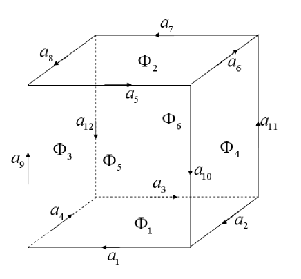
Figure 1: Magnetic flux $\Phi_{i}~{}(i=1,...,6)$ at the six boundaries and the integrals $a_{i}~{}(i=1,...,12)$ of $\int{\bf A}_{\rm p}\cdot\rm d{\bf l}$ at the twelve edges.

According to the Ampère’s law, the integral value $a_{i}$ satisfy the following linear equations

$${\rm{TX=B},}$$ (4)

where $\textrm{B}=(\Phi_{1},\Phi_{2},\Phi_{3},\Phi_{4},\Phi_{5},\Phi_{6})^{T}$, $\textrm{X}=(a_{1},a_{2},a_{3},...,a_{12})^{T}$ and T is a matrix of 6$\times$12 , which is equal

$$\left[\begin{array}[]{cccccccccccc}1&1&1&1&0&0&0&0&0&0&0&0\\ 0&0&0&0&1&1&1&1&0&0&0&0\\ 0&0&0&{-1}&0&0&0&{-1}&1&0&0&1\\ 0&{-1}&0&0&0&{-1}&0&0&0&1&1&0\\ {-1}&0&0&0&{-1}&0&0&0&{-1}&{-1}&0&0\\ 0&0&{-1}&0&0&0&{-1}&0&0&0&{-1}&{-1}\\ \end{array}\right].$$ (5)

One can check that the six rows-vector in this matrix is not linear independent because the magnetic field is divergence free and the sum of $\Phi_{i}$ at the six boundaries is zero. Moreover, the unknown twelve $a_{i}$ are not unique just under the restriction of above six conditions. Hence, we need to construct twelve independent conditions to obtain the unique solution for $a_{i}$. We define the new matrix $\hat{\textrm{T}}$ as follows

$$\left[\begin{array}[]{ccccccccccccc}1&1&1&1&0&0&0&0&0&0&0&0\\ 0&0&0&0&1&1&1&1&0&0&0&0\\ 0&0&0&{-1}&0&0&0&{-1}&1&0&0&1\\ 0&{-1}&0&0&0&{-1}&0&0&0&1&1&0\\ {-1}&0&0&0&{-1}&0&0&0&{-1}&{-1}&0&0\\ 1&0&{-1}&0&0&0&0&0&0&0&0&0\\ 0&1&0&{-1}&0&0&0&0&0&0&0&0\\ 0&0&1&0&{-1}&0&0&0&0&0&0&0\\ 0&0&0&1&0&{-1}&0&0&0&0&0&0\\ 0&0&0&0&1&0&{-1}&0&0&0&1&0\\ 0&0&0&0&0&1&0&{-1}&0&0&0&0\\ 0&0&0&0&0&0&1&0&{-1}&0&0&0\\ \end{array}\right].$$ (6)

One can check that the determinant of $\hat{\textrm{T}}$ is not zero. According to Cramer rule, the unique solution is existent for the new linear equation

$${\rm{{\hat{T}}X=\hat{B}},}$$ (7)

where $\textrm{X}=(a_{1},a_{2},a_{3},...,a_{12})^{T}$ and $\hat{\textrm{B}}=(\Phi_{1},\Phi_{2},\Phi_{3},\Phi_{4},\Phi_{5},0,0,0,0,0,0,0)^{T}$. Then we can obtain the integrals of $\int{\bf A}_{\rm p}\cdot\rm d{\bf l}$ at the twelve edges. The corresponding vector potential at the twelve edges could be obtained by using the following equation:

$$\begin{split}{\rm{A}}_{{\rm{px}}}\left({a_{i}}\right)=\frac{{\pi a_{i}}}{{2L_{x}}}\sin({{\pi x}\mathord{\left/{\vphantom{{\pi x}{L_{x}}}}\right.\kern-1.2pt}{L_{x}}}),i=1,3,5,7\\ {\rm{A}}_{{\rm{py}}}\left({a_{i}}\right)=\frac{{\pi a_{i}}}{{2L_{y}}}\sin({{\pi y}\mathord{\left/{\vphantom{{\pi y}{L_{y}}}}\right.\kern-1.2pt}{L_{y}}}),i=2,4,6,8\\ {\rm{A}}_{{\rm{pz}}}\left({a_{i}}\right)=\frac{{\pi a_{i}}}{{2L_{z}}}\sin({{\pi z}\mathord{\left/{\vphantom{{\pi z}{L_{z}}}}\right.\kern-1.2pt}{L_{z}}}),i=9,10,11,12\end{split}$$ (8)

Note that ${\bf A}_{\rm p}$ at the ends of every edge both are zero according to the above equation. That is the requirement of Eq. (2). Then we resolve the Poisson equations to obtain ${\bf A}_{\rm p}$ at the six boundaries. For the vector potential A at all boundaries the same values are taken as for ${\bf A}_{\rm p}$. Then we can follow the method of Sec. 2.2 and 2.3 of the former paper Yang et al. (2013) to calculate the relative magnetic helicity in this volume.

4 Testing the scheme

For testing the new scheme to obtain the vector potentials at the boundaries, we use the axisymmetric nonlinear force-free fields of Low and Lou (1990). We used the model labeled $P_{1,1}$ with $l=0.3$ and $\Phi=\pi/2$ in the notation of their paper. We calculated the magnetic field on a uniform grid of $64\times 64\times 64$. The pixel size in the calculation is assumed to be 1.

We calculate the magnetic fluxes $\Phi_{0}$ at the six boundaries and substitute it to the Eq. (7) to obtain the integral $a_{i}$ at the twelve edges of the 3D volume. Then we substitute $a_{i}$ into Eq. (8) respectively to get the boundary value for resolving the Poisson equation in Eq. (3) at the six boundaries. After we attain ${\bf A}_{\rm p}$ at the six boundaries, we could also calculate the magnetic flux $\Phi$ according to the relation between the vector potential and the magnetic field: ${\bf B}\cdot\hat{\rm n}=\nabla\times{\bf A}_{\rm p}\cdot\hat{\rm n}$. Table. 1 represents the final result after we apply the the above scheme. It can be found that the calculated magnetic fluxes at the six boundaries by using our scheme respectively coincide well with the original value from the theoretical model. Note that the total magnetic flux of the theoretical model is not exact zero. However, it is required that the total magnetic flux is exact zero when resolving the linear equation Eq. (7), which cause the total magnetic fluxes of $\oint{\bf A}_{\rm p}\cdot\rm d{\bf l}$ and $\Phi$ are different with that of $\Phi_{0}$. On the other hand, the numerical errors when resolving the Poisson equation are also unavoidable, which will also introduce the difference for the total magnetic flux as well.

Table 1: Testing using the new scheme to a theoretical model.

side boundary	$\Phi_{0}^{\tablenotemark{a}}$	$\oint{\bf A}_{\rm p}\cdot\rm d{\bf l}^{\tablenotemark{b}}$	$\Phi^{\tablenotemark{c}}$
$z=0$	-3615.81	-3615.81	-3487.1068
$z=l_{z}$	1461.13	1461.13	1490.2739
$x=0$	-1471.95	-1471.95	-1563.7657
$x=l_{x}$	-1471.95	-1471.96	-1564.9280
$y=0$	4006.42	4006.42	4087.8426
$y=l_{y}$	1068.27	1092.17	1066.6782
Total flux	-23.89	0.00012	28.99

5 Summary

In this paper, we propose a new scheme to calculate the vector potential at the boundaries to remove the restrictions in the former paper Yang et al. (2013). In principle, now we can calculate the relative magnetic helicity of any magnetic field structure in Cartesian coordinates. In the observations, we could use force-free extrapolation method to obtain the three-dimensional magnetic structure to analyze the evolution of relative magnetic helicity. On the other hand, we can also use a sequence of magnetograms to estimate the accumulated magnetic helicity in the solar corona (Ref. Démoulin and Pariat, 2009). It will be very interesting to compare the two types of accumulated magnetic helicity and analyze the correlation between magnetic helicity and solar eruption (e.g. Jing et al., 2012). In the simulations, we could also calculate the relative magnetic helicity directly based the known magnetic field structure to understand how the magnetic helicity plays an important role in solar reconnection and dynamos.

References

- Berger (1984) Berger, M. A., Field, G., B.: 1984, J. Fluid Mech. 147, 133.
- Berger (1999) Berger, M. A.: 1999, Plasma Phys. Contr. Fusion 41, 167.
- Boulmezaoud (1999) Boulmezaoud, T. Z.: 1999, Étude des champs de Beltrami dans des domaines de R3 bornś et non bornś et applications en astrophysique”, Ph.D. thesis, Univ. Paris VI.
- Démoulin and Pariat (2009) Démoulin, P., Pariat, E.: 2009, Adv. Space Res. 43, 1013.
- Jing et al. (2012) Jing, J., Park, S., Liu, C., Lee, J., Wiegelmann, T., Xu, Y., Deng, N., & Wang, H. M. : 2012, Astrophys. J. 752, L9
- Low and Lou (1990) Low, B. C., Lou, Y.Q.: 1990, Astrophys. J. 352, 343.
- Rudenko and Myshyakov (2011) Rudenko, G. V., Myshyakov, I. I.: 2011, Solar phys. 270, 165.
- Santos, Büchner, and Otto (2011) Santos, J. C., Büchner, J., Otto, A.: 2011, Astron. Astrophys. 535, A111.
- Seehafer, Kuzanyan, and Pipin (2003) Seehafer, N., Gellert, M., Kuzanyan, K. M., Pipin, V. V.: 2003, Adv. Space Res. 32, 1819.
- Thalmann, Inhester, Wiegelmann (2011) Thalmann, J. K., Inhester, B., Wiegelmann, T.: 2011, Solar Phys. 272, 243.
- Valori, Démoulin and Pariat (2012) Valori, G., Démoulin, P., Pariat, E.: 2012, Solar Phys. 278, 347.
- Woltjer (1958) Woltjer, L. 1958, Proc. Natl Acad. Sci. USA, 44, 480
- Santos et al. (2011) Santos, J. C., Büchner, J., & Otto, A. 2011, A&A, 535, A111
- Yang et al. (2013) Yang, S., Büchner, J. , Santos, J. C., & Zhang, H.: 2013, Solar Physics,283, 369.
- Yang, Büchner, and Zhang (2009a) Yang, S., Büchner, J., Zhang, H.: 2009, Astrophys. J. Lett. 695, L25.
- Yang, Büchner, and Zhang (2009b) Yang, S., Zhang, H., Büchner, J.: 2009, Astron. Astrophys. 502, 333.
- Zhang (2006) Zhang, H.: 2006, Astrophys. Space Sci. 305, 211.
- Zhang, Flyer, and Low (2006) Zhang, M., Flyer, M., Low, B.: 2006, Astrophys. J. 644, 575.