INFRARED BEHAVIOR OF SCALAR CONDENSATES IN EFFECTIVE HOLOGRAPHIC THEORIES

Abstract

We investigate the infrared behavior of the spectrum of scalar-dressed, asymptotically Anti de Sitter (AdS) black brane (BB) solutions of effective holographic models. These solutions describe scalar condensates in the dual field theories. We show that for zero charge density the ground state of these BBs must be degenerate with the AdS vacuum, must satisfy conformal boundary conditions for the scalar field and it is isolated from the continuous part of the spectrum. When a finite charge density is switched on, the ground state is not anymore isolated and the degeneracy is removed. Depending on the coupling functions, the new ground state may possibly be energetically preferred with respect to the extremal Reissner-Nordstrom AdS BB. We derive several properties of BBs near extremality and at finite temperature. As a check and illustration of our results we derive and discuss several analytic and numerical, BB solutions of Einstein-scalar-Maxwell AdS gravity with different coupling functions and different potentials. We also discuss how our results can be used for understanding holographic quantum critical points, in particular their stability and the associated quantum phase transitions leading to superconductivity or hyperscaling violation.

I Introduction

Holographic models have been widely used as a powerful tool to describe the strongly coupled regime of quantum field theory (QFT) Hartnoll et al. (2008a, b); Horowitz and Roberts (2008); Herzog (2009); Hartnoll (2009); Charmousis et al. (2009); Cadoni et al. (2010); Goldstein et al. (2010a); Gubser and Rocha (2010); Goldstein et al. (2010b); Charmousis et al. (2010); Bertoldi et al. (2010); Gouteraux and Kiritsis (2011); Iizuka et al. (2012); Cadoni and Pani (2011); Hartnoll (2011); Lee et al. (2011); Kim (2012); Dong et al. (2012); Wu and Zeng (2012); Hashimoto and Iizuka (2012); Ammon et al. (2012); Iizuka and Maeda (2012); Dey and Roy (2012); Park (2012); Myung and Moon (2012); Adam et al. (2013); Gouteraux and Kiritsis (2012). In the usual holographic setup, the $4$-dimensional gravitational bulk is described by an asymptotically anti-de Sitter (AdS) black brane (BB), generically sourced by a (neutral or charged) scalar field and by an electromagnetic (EM) field. The usual rules of the AdS/CFT correspondence are then used to describe a dual $3$-dimensional QFT at finite charge (or finite chemical potential) and where some scalar operator may acquire a nonvanishing expectation value. In particular, when the BB solution is sourced by a nontrivial scalar field configuration in the bulk, the dual QFT shows a (neutral or charged) scalar condensation.

These effective holographic theories (EHTs) have a wide range of applications. They have been used to give a holographic description of many interesting quantum phase transitions, such as those leading to critical superconductivity and hyperscaling violation Hartnoll et al. (2008a, b); Charmousis et al. (2009); Gubser and Rocha (2010); Cadoni et al. (2010); Goldstein et al. (2010a); Dong et al. (2012); Cadoni and Pani (2011); Cadoni and Mignemi (2012); Cadoni and Serra (2012). The properties of the QFT at small temperatures are essentially determined by the quantum phase transition at zero temperature. Thus, understanding the quantum critical point provides a full characterization of the thermodynamical phase transition at small temperatures.

If one assumes, as we do in this paper, that the asymptotic geometry is the AdS spacetime, the dual QFT shows a universal conformal fixed point in the ultraviolet (UV). The nontrivial dynamics therefore occurs in the infrared (IR) region, at the corresponding critical points. In a Wilsonian approach, EHTs should be first classified in terms of flows, driven by relevant operators, between critical points corresponding to scale-invariant (more generally scale-covariant) QFTs. Two other relevant characterizations of the critical points are: $a)$ the distinction between fractionalized phases (sourced by non-zero electric flux in the IR) and cohesive phases (sourced by zero electric flux in the IR); $b)$ phases with broken and unbroken $U(1)$ symmetry Hartnoll (2011); Gouteraux and Kiritsis (2012).

Progress in the classification and understanding of IR critical points have been achieved following various directions. In particular, it has been shown that in the case of hyperscaling preserving and hyperscaling violating solutions, quantum critical theories may appear as fixed lines rather than fixed points Gouteraux and Kiritsis (2012). Hyperscaling preserving solutions appear indeed as fixed points and correspond to AdS₄, AdS${}_{2}\times R^{2}$ and Lifshitz bulk geometries. However, hyperscaling violating solutions are characterized by an explicit scale and therefore appear rather as critical lines generated by changing that scale or equivalently the charge density Cadoni and Mignemi (2012); Cadoni and Serra (2012); Gouteraux and Kiritsis (2012); Dong et al. (2012).

A crucial point for understanding these quantum critical points is the presence of a scalar condensate. Indeed nontrivial configurations of (generically charged or uncharged) scalar fields play several crucial roles: (i) nontrivial scalar fields are dual to relevant operators that drive the renormalization group (RG) flow from the UV fixed point to the IR critical point (or line); (ii) scalar fields are the sources that support the IR hyperscaling violating geometry allowing for both fractionalized and cohesive phases Hartnoll (2011); Gouteraux and Kiritsis (2012); (iii) charged scalar condensates break the $U(1)$ symmetry and generate a superconducting phase Hartnoll (2011); Gouteraux and Kiritsis (2012).

Despite the recognized relevance of scalar condensates for describing holographic critical points, we are far from having a complete understanding of the physics behind them, in particular we have very few information about their stability. For instance, one would like to understand why at zero (and small) temperature the hyperscaling violating phase is energetically preferred with respect to the hyperscaling preserving phase. In this paper we will move a step forward in this direction by asking ourselves a simple, but relevant question: what is the energy of the ground state of a neutral asymptotically AdS BB sourced by a generic nontrivial scalar field? We show that for zero charge density the BB ground state must be degenerate with the AdS vacuum. This degeneracy is the result of an exact cancellation between a positive gravitational contribution to the energy and a negative contribution due to the scalar condensate.

Moreover, we also show that for the BB ground state the symmetries of the field equations force conformal boundary conditions for the scalar field, i.e. boundary conditions preserving the asymptotic symmetry group of the AdS spacetime. The conformal boundary conditions correspond to dual multitrace scalar operators driving the dynamics from the UV conformal fixed point to the IR critical point. In the case of an IR hyperscaling violating geometry sourced by a pure scalar field with a potential behaving exponentially, a scale is generated in the IR. On the other hand we will show that, in the case of pure Einstein-scalar gravity at finite temperature $T$, the boundary conditions for the scalar are determined by the dynamics and are, therefore, generically nonconformal. This means that the ground state for scalar BBs is isolated, i.e. it cannot be obtained as the $T\to 0$ limit of finite-$T$ BBs with conformal boundary conditions for the scalar field.

When a finite charge density $\rho$ is switched on, the degeneracy of the ground state is removed. Because an additional degree of freedom (the EM potential) is present, the boundary conditions for the scalar field are not anymore determined by the dynamics. The freedom in choosing the boundary conditions arbitrarily can be used to impose conformal boundary conditions also for BBs at finite temperature. The ground state for scalar BBs is therefore not anymore isolated from the continuous part of the spectrum. The coupling between the bulk scalar and EM field determines if it is energetically preferred with respect to the extremal Reissner-Nordstrom (RN) AdS BB.

We also derive several properties of the scalar BB near extremality and at finite temperature. For instance, we show that scalar-dressed, neutral (charged), BB solutions of radius $r_{h}$ (and charge density $\rho$) only exist for a temperature $T$ bigger than the temperature of the Schwarzschild-AdS (Reissner-Nordstrom AdS) BB with the same $r_{h}$ (and with the same $\rho$).

As a check and illustration of our results we give and discuss – both analytically and numerically – several (un)charged, scalar-dressed BB solutions of Einstein-scalar-Maxwell AdS (ESM-AdS) gravity with minimal, nonminimal and covariant coupling functions and different potentials (quadratic, quartic, exponential).

Finally, we also discuss the relevance of our results for understanding holographic quantum critical points, in particular their stability and the associated quantum phase transitions.

The structure of this paper is the following. In Sect. II we present the general form of the EHTs we consider. In Sect. III we investigate the spectrum of this class of theories in the IR region. In Sect. IV we derive extremal, near-extremal and finite-temperature BB solutions of pure Einstein-scalar gravity theories in the case of a quadratic, quartic and exponential potential. We also derive their thermodynamical behavior and their critical exponents. In Sect. V we derive and discuss charged solutions with the scalar minimally, nonminimally and covariantly coupled to the EM field. Finally in Sect. VI we end the paper with some concluding remarks about the relevance that our results have for understanding the dual QFT, holographic quantum critical points, in particular the stability of the latter and the associated quantum phase transitions leading to superconductivity or hyperscaling violation. In Appendix A we discuss perturbative solutions in the small scalar field limit.

II Effective holographic theories

We consider Einstein gravity coupled to a real scalar field and to an EM field in four dimensions:

$$I=\int d^{4}x\sqrt{-g}\left[R-\frac{1}{2}\left(\partial\phi\right)^{2}-\frac{Z(\phi)}{4}F^{2}-V(\phi)-Y(\phi)A^{2}\right].$$ (1)

where $F_{\mu\nu}=\partial_{\mu}A_{\nu}-\partial_{\nu}A_{\mu}$ is the Maxwell field-strength. The model is parametrized by the gauge coupling function $Z(\phi)$, by the self-interaction potential $V(\phi)$ for the scalar field and by the coupling function $Y(\phi)$ giving mass to the Maxwell field.

The action (1) defines ESM theories of gravity, which are also called EHTs and are relevant for holographic applications. EHTs have been widely used to give a holographical description of strongly-coupled QFTs with rich phenomenology such as quantum phase transitions, superconductivity and hyperscaling violation Hartnoll et al. (2008a, b); Charmousis et al. (2009); Gubser and Rocha (2010); Cadoni et al. (2010); Goldstein et al. (2010a); Dong et al. (2012); Cadoni and Pani (2011); Cadoni and Mignemi (2012); Cadoni and Serra (2012); Gouteraux and Kiritsis (2012). Moreover, models like (1) generically appear, after dimensional reduction, as low-energy effective string theories. The action (1) can be also interpreted as an EHT for a complex scalar field that enjoys a $U(1)$ symmetry Gouteraux and Kiritsis (2012). In this context the real scalar $\phi$ describes the modulus of the charged scalar and the phase with broken (unbroken) $U(1)$ symmetry is obtained by $Y\neq 0$ ($Y=0$).

Although our considerations can be easily extended to the case $Y\neq 0$, we will focus for simplicity on the case of unbroken $U(1)$ symmetry, $Y=0$. We will briefly comment on the case $Y\neq 0$ in Section V.3.

We are interested in electrically charged BB solutions of the theory, i.e. static solutions with radial symmetry for which the topology of the transverse space is planar. Using the following parametrization for the metric:

$$ds^{2}=-\lambda(r)dt^{2}+\frac{dr^{2}}{\lambda(r)}+H^{2}(r)(dx^{2}+dy^{2}),$$ (2)

the Einstein and scalar equations read:

$$\frac{H^{\prime\prime}}{H} = -\frac{(\phi^{\prime})^{2}}{4},\quad(\lambda H^{2})^{\prime\prime}=-2H^{2}V,$$ (3)

$$(\lambda HH^{\prime})^{\prime} = -H^{2}\left[\frac{V}{2}+\frac{ZA_{0}^{\prime}{}^{2}}{4}\right]\,,$$ (4)

$$(\lambda H^{2}\phi^{\prime})^{\prime} = H^{2}\left(\frac{dV}{d\phi}-\frac{A_{0}^{\prime}{}^{2}}{2}\frac{dZ}{d\phi}\right).$$ (5)

The ansatz (2) is very convenient, as in these coordinates Maxwell’s equations can be directly solved for $A_{0}^{\prime}$:

$$A_{0}^{\prime}=\frac{\rho}{ZH^{2}},$$ (6)

where $\rho$ is the charge density of the solution. Note that only Eqs. (4) and (5) depend on the EM field and only through $A_{0}^{\prime}$. Therefore, substituting the solution above into the remaining field equations, we can completely eliminate the EM field and solve Eqs. (3)–(5) for $\lambda$, $H$ and $\phi$.

We will consider models for which the potential $V(\phi)$ has a maximum at $\phi=0$ and $Z^{\prime}(\phi=0)=0$, with the local mass of the scalar $m_{s}^{2}=V^{\prime\prime}(0)$ satisfying the condition $m_{BF}^{2}<m_{s}^{2}\leq-2/L^{2}$ and with $V(0)=-6/L^{2}$, where $m_{BF}^{2}=-9/(4L^{2})$ is the Breitenlohner-Freedman (BF) bound Breitenlohner and Freedman (1982) in four dimensions and $L$ is the AdS length. The presence of an extremum of $V(\phi)$ and $Z(\phi)$ at $\phi=0$ implies the existence of a Reissner-Nordstrom-AdS (RN-AdS) BB solution,

$$\lambda=\frac{r^{2}}{L^{2}}-\frac{M}{2r}+\frac{\rho^{2}}{4r^{2}},\quad H=r,\quad\phi=0,$$ (7)

which is characterized by a trivial scalar field configuration.

On the other hand well-known “no-hair” theorems Torii et al. (2001); Hertog (2006); Cadoni et al. (2011, 2012) make the existence of BB solutions endowed with a nontrivial scalar field a rather involved question. Scalar-dressed solutions are particularly important for holographic applications because they describe dual QFTs with a scalar condensate.

The AdS, $r=\infty$, asymptotic behavior requires the following leading behavior of the metric and the scalar field:

$$ds^{2} = -\frac{r^{2}}{L^{2}}dt^{2}+\frac{L^{2}}{r^{2}}dr^{2}+r^{2}(dx^{2}+dy^{2})$$

$$\phi = \frac{O_{1}}{r^{\Delta_{1}}}+\frac{O_{2}}{r^{\Delta_{2}}},$$ (8)

with $\Delta_{1,2}=\frac{3\mp\sqrt{9+4m_{s}^{2}L^{2}}}{2}$. Because the AdS spacetime is not globally hyperbolic, this asymptotic behavior must be supported by boundary conditions on $O_{1}$, $O_{2}$. Dirichlet boundary conditions that preserve the asymptotic isometries of the AdS spacetime are $O_{1}=0$. However, in the range of scalar masses $m_{BF}^{2}<m_{s}^{2}<m_{BF}^{2}+1/L^{2}$, boundary conditions of the form ($f$ is a constant):

$$O_{1}=fO_{2}^{\Delta_{1}/\Delta_{2}},$$ (9)

which preserve the conformal, asymptotic symmetries of the AdS background, are also allowed Hertog and Maeda (2004). More in general, boundary conditions of the form

$$O_{1}=W(O_{2}),$$ (10)

can be used. For a generic form of the function $W$ the asymptotic AdS isometries are broken, yet an asymptotic time-like Killing vector exists and the gravitational theory admits a dual description in terms of multitrace deformations of CFTs Witten (2001); Aharony et al. (2001); Berkooz et al. (2002); Marolf and Ross (2006); Hartman and Rastelli (2008); Vecchi (2011); Hertog and Horowitz (2005).

Apart from their UV AdS behavior, the scalar-dressed solutions of EHTs are also characterized by their, small $r$, IR behavior. This IR behavior is of crucial relevance for holographic applications, in particular in the context of the AdS/Condensed Matter correspondence Hartnoll (2009). Generically, we expect the IR regime not to be universal, but rather determined by the infrared behavior of the potential $V(\phi)$ and of the gauge coupling functions $Z(\phi)$, $Y(\phi)$. Nevertheless, we will discover in the next sections some features of the IR spectrum of EHTs, which are model-independent and related to the scaling symmetries of the UV AdS vacuum.

Although we will be concerned with general features of EHTs, for the sake of definiteness we will mainly focus on three classes of models with different IR behavior of the potential $V(\phi)$:

• The potential has a quadratic form

  $$V(\phi)=-\frac{6}{L^{2}}+\frac{m_{s}^{2}\phi^{2}}{2}.$$ (11)

  This corresponds to the simplest choice for the potential, which has been widely used in holographic models. The IR regime is dominated by the quadratic term and at $T=0$ the scalar field diverges logarithmically in the $r=0$, near-horizon region.

• The potential behaves exponentially for small values of the radial coordinate $r$. Assuming that $r=0$ corresponds to $\phi\rightarrow\infty$, we have in this case

  $$V(\phi)\sim e^{b\phi},$$ (12)

  where $b$ is a positive constant. As we shall discuss later in Sect. IV.3, this case produces a scale-covariant solution in the IR, corresponding to hyperscaling violation in the dual QFT.

• The origin $r=0$ corresponds to an other extrema (a minimum) at $\phi=\phi_{1}$ of the potential $V(\phi)$. In this case the theory flows to a second AdS₄ vacuum in the infrared.

The IR regime of the EHT (1) is also characterized by the IR behavior of the gauge coupling function $Z$. In particular, $Z$ is crucial for determining the contribution of bulk degrees of freedom inside or outside the event horizon to the boundary charge density. This distinction is captured by the behavior of the electric flux in the IR

$$\Phi=\left(\int_{R^{2}}Z(\phi)\tilde{F}\right)_{\mathrm{IR}},$$ (13)

where $\tilde{F}$ is the dual Maxwell tensor. Using a terminology borrowed from condensed matter physics, the phase with $\Phi=0$ has been called cohesive and describes dual confined gauge invariant operators. The phase $\Phi\neq 0$ has been named fractionalized and describes a dual deconfined phase Hartnoll (2011); Gouteraux and Kiritsis (2012). In this paper we will consider two choices for the gauge coupling function $Z(\phi)$: $(1)$ a minimal coupling, $Z(\phi)=1$; $(2)$ a coupling which behaves exponentially in the IR, $Z\sim e^{a\phi}$.

Since in the following we shall make often use of the thermodynamical properties of the BB solutions, we find it convenient to summarize them here. The temperature $T$, entropy $S$ and free energy $F$ of the solutions (2) are given by

$$T=\frac{\lambda^{\prime}(r_{h})}{4\pi}\,,\qquad S=4\pi\mathcal{V}H^{2}(r_{h}),\text{ \ \ \ \ \ }F=M-TS,$$ (14)

where $M$ is the total mass of the solution, $\mathcal{V}$ is the volume of the $2D$ sections of the spacetime and $r_{h}$ is the location of the outer event horizon.

III Spectrum of Einstein-Scalar-Maxwell AdS gravity in the Infrared region

In this section we investigate general features of the mass spectrum of ESM-AdS gravity in the IR region. Assuming the existence of scalar-dressed BBs with AdS asymptotic behavior, the two basic questions in this context are about the existence and features of the $T=0$ extremal state and of the states near-extremality. We will treat separately the EM charged and uncharged cases. We will first consider the theory with zero charge density ($Z=Y=0$ in the action (1)), i.e. a vanishing Maxwell field (Einstein-scalar AdS gravity). Later, we will extend our considerations to the case of finite charge density.

III.1 Einstein-Scalar AdS gravity

A nontrivial point is the determination of the total mass $M$ (i.e. the energy) of the BB solution. As discussed in Ref. Hertog and Horowitz (2005), the usual definition of energy in AdS diverges whenever $O_{1}\neq 0$ (with a divergent term proportional to $r$). This is because the backreaction of the scalar field causes certain metric components to fall off slower than usual. However, this divergent term is exactly canceled out if one considers that for $O_{1}\neq 0$ there is an additional scalar contribution to the surface terms which determines the mass.

Using the Euclidean action formalism in the case $m_{s}^{2}=-2/L^{2}$ the total mass turns out to be Hertog and Horowitz (2005)

$$M=M_{G}+\frac{\mathcal{V}}{L^{4}}\left[O_{1}O_{2}+P(O_{1})\right],$$ (15)

where $M_{G}$ is the gravitational contribution to the mass, we have chosen the following boundary conditions for the scalar: $O_{2}=O_{2}(O_{1})$, and $P(O_{1})=\int O_{2}(O_{1})dO_{1}$.

In the following we will need an expression for the mass when $m_{s}$ is in the range of values considered in this paper, $-9/4<m_{s}^{2}L^{2}\leq-2$. Furthermore, working with the parametrization of the metric given by Eq. (2), it is useful to express the total mass $M$ in terms of the coefficient of the $1/r$ term in the $r=\infty$ expansion of the metric functions. To derive such an expression we use the Euclidean action formalism of Martinez et al. Martinez et al. (2004). Using the parametrization of the metric (2) the gravitational and scalar part of the variation of the boundary terms are given respectively by Martinez et al. (2004):

$$\delta I_{G} = \frac{2\mathcal{V}}{T}\left[(HH^{\prime}\delta\lambda-\lambda^{\prime}H\delta H)+2\lambda H(\delta H^{\prime})\right]|_{r_{h}}^{\infty},$$

$$\delta I_{\phi} = \frac{\mathcal{V}}{T}H^{2}\lambda\phi^{\prime}\delta\phi|_{r_{h}}^{\infty}.$$ (16)

From the definition of the free energy $F=M-TS$, taking into account that $I_{\phi}|_{r_{h}}=0,\,S=I_{G}|_{r_{h}}$ and from $F=-IT$, it follows

$$M=TS-TI=-T(I_{G}^{\infty}+I_{\phi}^{\infty}).$$ (17)

To calculate the mass $M$ (17) we need the subleading terms in the $r=\infty$ expansion of the metric (II). By means of a translation of the radial coordinate $r$, the asymptotic expansion of the solution can be put in the general form:

$$\lambda = \frac{r^{2}}{L^{2}}+pr^{\beta}-\frac{m_{0}}{2r}+{\mathcal{O}}({r^{\beta-1}}),$$

$$H^{2} = \frac{r^{2}}{L^{2}}+qr^{\alpha}+\frac{s}{r}+{\mathcal{O}}({r^{\alpha-1}}),$$

$$\phi = \frac{O_{1}}{r^{\Delta_{1}}}+\frac{O_{2}}{r^{\Delta_{2}}}+{\mathcal{O}}({r^{-\Delta_{1}-1}}),$$ (18)

where $p,q,\alpha,\beta,s$ are constants. Inserting this expansion in the field equations one gets (at the first and second subleading order) the following relations between the constants:

$$\beta=\alpha=2(1-\Delta_{1}),\quad p=q=\frac{\Delta_{1}O_{1}^{2}}{4L^{2}(1-2\Delta_{1})},\quad s=-\frac{\Delta_{1}\Delta_{2}O_{1}O_{2}}{6L^{2}}.$$ (19)

Substituting Eq. (III.1) into (III.1) and using $p=q$, we obtain

$$\delta I_{G}^{\infty} = -\frac{\mathcal{V}}{TL^{2}}\left(\delta m_{0}+6\delta s-2\delta p(\beta-1)r^{\beta+1}\right)\,,$$ (20)

$$\quad\delta I_{\phi}^{\infty} = -\frac{\mathcal{V}}{TL^{4}}\left(\Delta_{1}O_{1}\delta O_{1}r^{\beta+1}+\Delta_{1}O_{1}\delta O_{2}+\Delta_{2}O_{2}\delta O_{1}\right)\,.$$ (21)

Notice that both the gravitational and the scalar contribution to the mass contain a term which diverges as $r^{\beta+1}$. Using Eq. (19) one easily finds that the two divergent terms cancel out in $\delta I^{\infty}=\delta I_{G}^{\infty}+\delta I_{\phi}^{\infty}$ . Finally, we obtain the total mass of the solution

$$M=-TI^{\infty}=\frac{\mathcal{V}}{L^{2}}\left(m_{0}+\frac{(\Delta_{1}-\Delta_{2})}{L^{2}}\int dO_{2}W(O_{2})+\frac{\Delta_{2}(1-\Delta_{1})}{L^{2}}O_{2}O_{1}\right),$$ (22)

where we have parametrized the boundary conditions for the scalar in terms of the function $O_{1}=W(O_{2})$. It is also useful to split the total mass into the gravitational and scalar contributions $M_{G}$ and $M_{\phi}$, arising separately from the two terms in Eq. (22):

$$M_{G}=\frac{\mathcal{V}}{L^{2}}\left(m_{0}-\frac{\Delta_{1}\Delta_{2}}{L^{2}}O_{1}O_{2}\right),\quad M_{\phi}=\frac{\mathcal{V}}{L^{4}}\left[\Delta_{1}O_{1}O_{2}+(\Delta_{2}-\Delta_{1})P(O_{1})\right],$$ (23)

where $P(O_{1})$ is defined as in Eq. (15). One can easily check that the previous equations reproduce correctly Eq. (15) in the case $m_{s}^{2}=-2/L^{2}$, i.e. $\Delta_{1}=1,\Delta_{2}=2$.

Let us now investigate general features of the mass spectrum of ES-AdS gravity in the IR region. In particular, assuming the existence of scalar-dressed BBs with AdS asymptotic behavior, we wish to characterize the features of the $T=0$ extremal state and of the near-extremal states.

In the uncharged case a general, albeit implicit, form of the solution for the metric function $\lambda$ in a generic ES-AdS gravity theory has been derived in Ref. Cadoni et al. (2011):

$$\lambda=H^{2}-C_{1}H^{2}\int\frac{dr}{H^{4}},$$ (24)

where $C_{1}$ is an integration constant. The equation above implies that if an extremal $T=0$ hairy BB solution exists, this must have $C_{1}=0$, i.e. $\lambda=H^{2}$. We can prove this statement by the following argument. Differentiating the equation above and using Eqs. (14), we find the following relation between the temperature and the entropy density $\mathcal{S}$ of the solution:

$$T=\frac{\lambda^{\prime}(r_{h})}{4\pi}=\frac{\left(2\lambda HH^{\prime}-C_{1}\right)_{r_{h}}}{{\mathcal{S}}}.$$ (25)

Therefore we get $C_{1}=\left[2\lambda HH^{\prime}\right]_{r_{h}}-\mathcal{S}T$. An extremal solution satisfies $T=0$ and $\lambda(r_{h})=0$. Assuming that $H$ and $H^{\prime}$ are finite at the horizon (to avoid curvature singularities), the existence of an extremal solution imposes $C_{1}=0$, i.e.

$$\lambda=H^{2}.$$ (26)

Note that this argument applies both when the entropy of the extremal solution is vanishing or when it is finite.

Obviously, an extremal uncharged solution with AdS asymptotics (besides the trivial AdS vacuum) may not exist. For the moment, we assume such a solution exists and derive a general and very important result. We shall prove that if such a solution exists it must have zero energy, i.e. must be degenerate with the AdS vacuum.

To prove this statement, let us first show that every scalar-dressed solution with AdS asymptotics, which is characterized by $\lambda=H^{2}$, requires necessarily conformal boundary conditions (9) for the scalar field. The field equations (3)–(6) with $\rho=0$ and the metric (2) are invariant under the scale transformation $r\rightarrow\mu r,\,\lambda\rightarrow\mu^{2}\lambda,\,t\rightarrow\mu^{-2}t$. In the extremal case, the asymptotic expansion (III.1) implies that full solution ($\lambda=H^{2}$ and $\phi$) is invariant under this scale transformation if $O_{1,2}$ scale as follows: $O_{1}\rightarrow\mu^{\Delta_{1}}O_{1},\,O_{2}\rightarrow\mu^{\Delta_{2}}O_{2}$, which in turn implies the conformal boundary condition (9).

We can now calculate the mass (22) of the extremal solution, which has $\lambda=H^{2}$, hence $m_{0}=-2s$. We get,

$$M=\frac{\mathcal{V}}{L^{4}}\left[(\Delta_{2}-\Delta_{1})P(O_{1})+\Delta_{1}(1-\frac{2}{3}\Delta_{2})O_{2}O_{1}\right],$$ (27)

where $P(O_{1})$ is defined as in Eq. (15). From Eq. (27) it follows almost immediately that for conformal boundary conditions (9) the mass $M$ vanishes.

This is an important and extremely nontrivial result. It means that in ES-AdS gravity with no EM field, if an extremal scalar-dressed BB solution exists then the AdS₄ vacuum of the theory must necessarily be degenerate. Physically, this degeneration is a consequence of the fact that the scalar condensate gives a negative contribution to the energy. Therefore we may have configurations in which the positive gravitational energy is exactly canceled by the negative energy of the scalar condensate. This cancellation is a consequence of the conformal symmetry of the extremal solution; it necessarily occurs because the extremality condition $\lambda=H^{2}$ forces the conformal boundary conditions (9).

It is also important to notice that the argument leading to the degeneracy of the $T=0$ ground state holds true also when a condition much weaker than Eq. (26) is satisfied:

$$\lambda=H^{2}+{\mathcal{O}}(r^{-2}).$$ (28)

In fact the mass (22) and the scaling arguments leading to the conformal boundary conditions for the scalar field depend only on terms up to ${\mathcal{O}}(r^{-1})$ and are completely insensitive to higher order terms in $1/r$.

Let us now consider near-extremal solutions. We assume that the theory allows for scalar-dressed BBs at finite temperature with AdS asymptotics. In the next section, we shall prove the existence of finite temperature solutions, by constructing AdS-BBs, numerically, for three classes of ES-AdS gravity models.

The BB spectrum near-extremality can be investigated by considering the $T\rightarrow 0$ limit of the finite $T$ solutions. However, one can show that this $T\rightarrow 0$ limit is singular. In order to prove the statement we expand the fields in the near-horizon region,

$$\lambda=\sum_{n=1}^{\infty}a_{n}(r-r_{h})^{n},\quad H=\sum_{n=0}^{\infty}b_{n}(r-r_{h})^{n},\quad\phi=\sum_{n=0}^{\infty}c_{n}(r-r_{h})^{n}\,.$$ (29)

At first order we get for $b_{0}\neq 0$

$$b_{2}=-\frac{b_{0}}{4}c_{1}^{2},\quad b_{1}a_{1}=-\frac{b_{0}}{2}V(c_{0}),\quad a_{1}c_{1}=\left(\frac{dV}{d\phi}\right)_{c_{0}},$$ (30)

whereas the temperature of the dressed solutions, from Eq. (14), becomes

$$T=\frac{a_{1}}{4\pi}=-\frac{b_{0}V(c_{0})}{8\pi b_{1}}\,.$$ (31)

Because in the case under consideration ($V$ has a maximum) the potential $V$ is limited from above ($V(\phi)\leq-6/L^{2}$), the $T\rightarrow 0$ limit can only reached by letting $b_{0}\rightarrow 0$. But on the other hand from the third equation in (30) it follows immediately that $a_{1}=0$ is a singular point of the perturbative expansion (29) unless $(dV/d\phi)_{c_{0}}=0$ (corresponding to the Schwarzschild-anti de Sitter (SAdS) BB). Thus the $T\rightarrow 0$ limit is a singular point of the perturbation theory. It should be stressed that this result has been derived by first considering the near-horizon limit, then taking $T\rightarrow 0$. In section IV.4 we will see what happens if the two limits are taken in the reversed order.

Note that the above results are strictly true only if one considers AdS solutions with negative mass squared for the scalar field. If the scalar potential has a local minimum at $\phi=0$, then our argument above does not apply. This is for instance the case with the class of models studied in Ref. Cadoni et al. (2012) which, however, turn out not to have BB solutions with AdS asymptotics.

The singularity of the $T\to 0$ limit in the near-horizon perturbation theory, indicates that the ground state (26) is isolated, i.e. it cannot be reached as the $T\to 0$ limit of finite$-T$ scalar BB solutions. This conclusion can be also inferred by reasoning on the $r=\infty$ boundary conditions for the scalar field. We have previously shown that the symmetries of the field equations together with Eq. (26) force conformal boundary conditions (9) for the scalar field. On the other hand, one can easily show that in the case of $T$ finite, the field equations together with the conditions for the existence on an event horizon imply boundary conditions of the form (10), hence in general nonconformal boundary conditions. In fact, the field equations (3)–(6) have the following symmetries:

$$r\rightarrow kr,\quad t\rightarrow kt,\quad L\rightarrow kL,\quad H\rightarrow kH$$

$$r\rightarrow kr,\quad\lambda\rightarrow k^{2}\lambda,\quad t\rightarrow k^{-1}t,\quad A_{0}\rightarrow kA_{0}$$ (32)

$$H\rightarrow kH,\quad(x,y)\rightarrow k^{-1}(x,y),$$

$$\lambda\rightarrow k\lambda,\quad t\rightarrow k^{-1}t,\quad H^{2}\rightarrow k^{-1}H^{2},\quad L\rightarrow kL\,,\quad A_{0}^{2}\rightarrow k^{-1}A_{0}^{2}$$

These symmetries can be used to fix all but one parameter in the perturbative expansion (29). The solutions become in this way a one-parameter family of solutions. The near-horizon expansion (29) depends on a single free parameter, which can be chosen to be $r_{h}$. For each value of $r_{h}$, we can extract the two functions $O_{1}(r_{h})$ and $O_{2}(r_{h})$, which define implicitly the boundary condition $O_{1}=W(O_{2})$.

It follows that in general the finite$-T$ solution require boundary conditions for the scalar, which are different from the conformal ones required for the ground state (26). Therefore, the solution (26) is generically isolated, i.e. it cannot be reached as the $T\to 0$ limit of finite$-T$ scalar BB solutions.

It should be stressed that the above feature is a key general feature of the BB solutions of AdS Einstein-scalar gravity which holds true also for the numerical solutions discussed in the next sections. If one assumes an analytic expansion close to the horizon, an asymptotically AdS behavior at infinity and if one requires the existence of hairy BB solutions, then the boundary conditions at infinity cannot be arbitrarily imposed but are determined by the field equations. These boundary conditions will have the form (10), with the function $W$ determined by the dynamics. In the dual QFT the function $W$ characterizes the scalar condensate. Thus, the particular form of the condensate is determined by the gravitational dynamics. It is obvious that this is true only in the case of pure Einstein-scalar gravity. For instance it does not hold for electrically charged solutions. In this latter case the near-horizon solution has always more than one free parameter, that can be fixed by prescribing some boundary condition for the scalar field.

We can also compare the temperature of the dressed solution of radius $r_{h}$ with the temperature $T_{0}$ of the SAdS BB with the same radius. We can use Eqs. (III.1) to set $r_{h}=L$,$\,b_{1}=c_{1}=L^{-1},b_{0}=1$, so that the only free parameter is $c_{0}=\phi(r_{h})$ and the temperature becomes $-8\pi T=LV(c_{0})$. We have therefore

$$T-T_{0}=8\pi L(V(0)-V(c_{0})\,).$$ (33)

In the case under consideration, $V(\phi)$ has a local maximum at $\phi=0$, so that $V(0)\geq V(c_{0})$. Therefore, we obtain $T>T_{0}$ for any finite temperature solution. That is, there exists a critical temperature given by the temperature of the SAdS BB: $T_{0}=\frac{3r_{h}}{4\pi L^{2}}$ such that scalar-dressed solutions of the same radius $r_{h}$ only exist when $T>T_{0}$.

III.2 Einstein-Scalar-Maxwell AdS gravity

Let us now consider the EM charged case, i.e. a finite charge density in the dual QFT. In general, one expects that the finite charge density will remove the degeneracy of the $T=0$ extremal state we have found in the uncharged case. This can be shown explicitly. Indeed, when $\rho\neq 0$, the field equations imply

$$\frac{\rho^{2}}{ZH^{2}}+2\lambda{H^{\prime}}^{2}+2\lambda HH^{\prime\prime}=H^{2}\lambda^{\prime\prime}\,,$$ (34)

which is solved by Eq. (24) only when the charge is vanishing. In particular, $\lambda=H^{2}$ is not a solution of the equation above when $\rho\neq 0$. Moreover in the charged case Eq. (24) becomes Cadoni et al. (2011)

$$\lambda=H^{2}\left[1-C_{1}\int\frac{dr}{H^{4}}+\rho^{2}\int dr\left(\frac{1}{H^{4}}\int\frac{dr}{ZH^{2}}\right)\right].$$ (35)

By using the same procedure leading to Eq. (26), we get that the extremal solution in the EM charged case is attained for

$$C_{1}=\rho^{2}\left(\int\frac{dr}{ZH^{2}}\right)_{r_{h}}.$$ (36)

Because $C_{1}\neq 0$, not even the weaker condition (28) is satisfied in the charged case. This implies that Eq. (27) does not hold if $\rho\neq 0$. In general, the mass of the extremal scalar-dressed solution will be different from the mass of the extremal RN-AdS solution, so that the degeneration of the $T=0$ ground state in the EM charged case is removed.

Notice that in the charged case the $T=0$ solution is not necessarily forced to have conformal boundary conditions for the scalar field. In fact, the argument used for the uncharged case is based both on the relation $\lambda=H^{2}$ and on the scale symmetries of the field equations. Both do not hold anymore at finite charge density. Nevertheless, in this case the presence of an additional field (the EM potential $A_{\mu}$) allows to choose arbitrary boundary conditions for the scalar. As discussed in the previous section, the boundary conditions are not anymore imposed by the dynamics of the system as in the uncharged case. It follows that in the charged case the $T=0$ ground state is not anymore isolated but can be reached continuously as the $T=0$ limit of finite temperature scalar dressed BB solutions.

For what concerns the BB spectrum near extremality, the results we have found in the uncharged case still hold in the charged case. In fact the first and the third equation in (30) are not modified by the nonvanishing charge, whereas the second becomes $a_{1}b_{1}=-(Z^{-1}(c_{0})\rho^{2}+2b_{0}^{4}V(c_{0}))/4b_{0}^{3}$. We obtain the temperature:

$$T=\frac{a_{1}}{4\pi}=-\frac{Z^{-1}(c_{0})\rho^{2}+2b_{0}^{4}V(c_{0})}{16\pi b_{1}b_{0}^{3}}\,.$$ (37)

Also here, we can compare the temperature of a scalar-dressed BB with that of the RN BB with the same charge $\rho$ and radius $r_{h}$. One easily finds that Eq. (33) still holds for the charged case and that $T>T_{0}^{RN}$ for any finite temperature solution, where the critical temperature $T_{0}^{RN}$ is given by

$$T_{0}^{RN}=\frac{12r_{h}^{4}-L^{2}Z^{-1}(c_{0})\rho^{2}}{16\pi r_{h}^{3}L^{2}}\,.$$ (38)

Scalar dressed EM charged solutions of the same radius $r_{h}$ and charge of the RN-AdS solution exist only for $T>T_{0}^{RN}$.

An important issue when dealing with finite EM charge density is the characterization of the phase as fractionalized or cohesive Hartnoll (2011); Gouteraux and Kiritsis (2012). For the generic theory (1) with $Y\neq 0$, this characterization will depend on the IR behavior of both $Z(\phi)$ and $Y(\phi)$. However, one can easily show that in the case of unbroken $U(1)$ symmetry, $Y=0$, only the fractionalized phase may exist. In fact using Eq. (6) into Eq. (13) one easily finds $\Phi\sim\rho$.

To summarize, the following interesting picture emerges for the IR spectrum of scalar-dressed BB solutions of ESM-AdS gravity with $m_{BF}^{2}<m_{s}^{2}<m_{BF}^{2}+1/L^{2}$. If a scalar-dressed, neutral, extremal solution exists at $\rho=0$, it must necessarily be degenerate with the AdS vacuum. This is due to a precise cancellation of the contributions to the total energy from the gravitational and scalar part and, in turn, it is due to the conformal symmetries of the boundary theory. Moreover, the $T\rightarrow 0$ limit of finite-$T$ BB solution is singular and the ground state is isolated from the continuous part of the spectrum.

When an EM charge is switched on, the degeneracy of the ground state is removed and the ground state can be reached continuously as the $T\to 0$ limit of finite$-T$ solutions. Scalar dressed uncharged (EM charged) solutions of the same radius $r_{h}$ (and charge) of S-AdS (RN-AdS) solution exist only for $T>T_{0}$ ($T>T_{0}^{RN}$). Cohesive phases may exist only when the $U(1)$ symmetry is broken. In the $U(1)$ symmetry-preserving case only the fractionalized phases are allowed.

Our results are fairly general and only assume the existence of scalar dressed solutions, which has to be investigated numerically. In the next two sections we will show that the picture above is realized for three wide classes of models with quadratic, quartic and exponential potentials $V(\phi)$ and for two classes of gauge couplings ($Z=1$ and $Z\sim e^{a\phi}$). Numerical computations confirms the degeneracy of the ground state in the uncharged case and the peculiarity of the $T\rightarrow 0$ limit of finite-temperature scalar-dressed BB solutions. We will discuss separately the EM neutral and charged solutions.

IV Neutral solutions

IV.1 Quadratic potential

In this section we will construct numerical solutions of ES-AdS gravity models with the quadratic potential (11) and we shall check the validity of the general results of Section III. The case of a quadratic potential is the simplest possible choice and it is therefore our first example. Moreover, this is the usual choice for models describing holographic superconductors. We will come back to this point later in Sect. V.3.

IV.1.1 Extremal solutions

The near-horizon behavior of the extremal solution of the model (11) with an EM field covariantly coupled to a charged scalar field has been derived in Ref. Horowitz and Roberts (2009). The near-horizon, extremal solution of a pure Einstein-scalar gravity model (both the EM and the charge of the scalar field are zero) can be obtained as a particular case of the solution given in Ref. Horowitz and Roberts (2009). In the gravitational gauge used in Ref. Horowitz and Roberts (2009), we have

$$ds^{2}=-g(\hat{r})e^{-\chi}dt^{2}+\frac{d\hat{r}^{2}}{g(\hat{r})}+\hat{r}^{2}(dx^{2}+dy^{2}),$$ (39)

and with our normalization for the kinetic term of the scalar field, the solution reads

$$ds^{2}=\frac{d\hat{r}^{2}}{g_{0}\hat{r}^{2}(-\ln\hat{r})}+\hat{r}^{2}(-dt^{2}+dx^{2}+dy^{2}),\quad\phi=2\sqrt{2}(-\ln\hat{r})^{1/2},\quad g_{0}=-\frac{2m_{s}^{2}}{3}.$$ (40)

The near-horizon, extremal solution (40) can be written in the gauge (2) by a suitable reparametrization of the radial coordinate. We get

$$\lambda=H^{2}=e^{-\frac{g_{0}X^{2}(r)}{2}},\quad\phi=-\sqrt{2g_{0}}\,X(r),\quad r=\sqrt{\frac{\pi}{g_{0}}}+\int^{X}dte^{-\frac{g_{0}t^{2}}{4}},$$ (41)

where the last equation defines implicitly the function $X(r)$. We note that also in these coordinates the horizon is located at $r={0}$.

The global, extremal, solution interpolating between the near-horizon behavior (41) and the asymptotic AdS behavior (III.1) has to be found numerically. We have integrated the field equations numerically for several values of $m_{s}^{2}$. In all cases we have found $\lambda=H^{2}$, which implies the conformal boundary condition (9). Indeed the total mass $M$ of the scalar-dressed solution is zero. In Fig. 1 we show the profiles of the metric functions and the scalar field for $m_{s}^{2}=-2/L^{2}$.

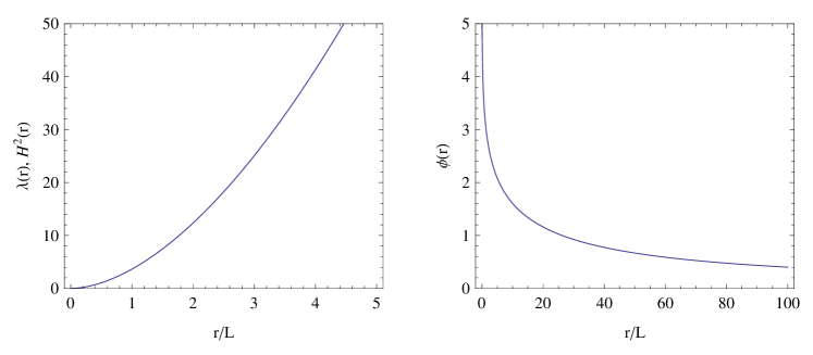
Figure 1: The metric functions $\lambda=H^{2}$ (left) and the scalar field $\phi$ (right) as functions of $r/L$, in the extremal case, for a quadratic potential with $m^{2}_{s}L^{2}=-2$.

IV.1.2 Finite-temperature solutions

Let us now consider BB solutions of Einstein-scalar theory at finite temperature. Again we have to construct global solutions, which interpolate between the asymptotic AdS expansion given by Eq. (III.1) and a near-horizon expansion as in Eq. (29).

We have constructed these solutions numerically, starting from the near-horizon solution above and integrating outwards to infinity, where the asymptotic behavior of the solution is AdS₄. In Fig. 2 we show an example of the metric and scalar profiles and of the function $O_{2}(O_{1})$ in the case $m_{s}^{2}=-2/L^{2}$ . In the large $O_{1}$ limit, our data are well fitted by $O_{2}\sim-0.57O_{1}^{2}$, which is consistent with the conformal boundary condition (9). However, for small values of $O_{1}$ the behavior reads $O_{2}\sim-0.36O_{1}$ and the global behavior interpolates between these two asymptotic regimes. Therefore, the function $O_{2}(O_{1})$ does not generically satisfy the conformal boundary conditions (9). This is a general statement that we have verified also for different choices of the parameters and different models. This fact confirms that extremal solution are isolated from finite temperature solutions.

As expected, solutions dressed with scalar hairs only exist above a certain critical temperature $T_{0}=3/(4\pi)$ and a critical mass $M_{0}$ which correspond to the temperature and mass of the Schwarzschild-AdS BB after a rescaling that sets $r_{h}=L=1$. This is shown in Fig. 3, where we present the total mass $M$ of the solutions as a function of the temperature $T$. The absence of dressed solutions (irrespectively of the boundary conditions $O_{2}(O_{1})$) for $T<T_{0}$ confirms numerically the existence of the critical temperature $T_{0}$.

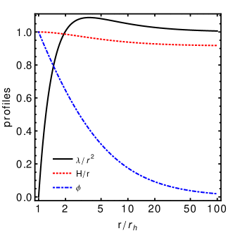
Figure 2: Left panel: metric and scalar profiles as functions of the (nonrescaled) coordinate $r$ for a quadratic potential with $m^{2}_{s}L^{2}=-2$. Right panel: the function $O_{2}=O_{2}(O_{1})$ for the same model.

Figure 3: Total mass $M$ as a function of the temperature $T$ for a quadratic potential with $m^{2}_{s}L^{2}=-2$.

IV.2 Quartic potentials

In this section we will check numerically the results of Section III, and the validity of the picture that has emerged from our results, in the case of a theory with a potential $V(\phi)$ having the behavior described as type $c)$ in Section II, i.e. a theory with a IR fixed point. As an example of such a theory we take the quartic potential,

$$V(\phi)=\Lambda^{4}\phi^{4}-\frac{\hat{m}^{2}}{2}\phi^{2}-\frac{6}{L^{2}}.$$ (42)

This potential has the typical mexican hat form with a maximum at $\phi=0$ with $V(0)=-6/L^{2},\,V^{\prime\prime}(0)=-\hat{m}^{2}$ and a minimum at $\phi_{12}=\pm\frac{\hat{m}}{2\Lambda^{2}}$ with $V(\phi_{1})=-6/l^{2}=-\hat{m}^{4}/(16\Lambda^{4})-6/L^{2},\,V^{\prime\prime}(\phi_{1})=2\hat{m}^{2}$. The potential is invariant under the discrete transformation $\phi\rightarrow-\phi$, so that we will just consider $\phi\geq 0$. The theory allows for two AdS₄ vacua: an UV AdS at $\phi=0$ (corresponding to $r=\infty$), with AdS length $L$ and with squared mass of the scalar given by $-\hat{m}^{2}$, and an IR $AdS_{4}$ at $\phi=\phi_{1}$ (corresponding to $r=0$) with AdS length $l$ and with squared mass of the scalar given by $2\hat{m}^{2}$. Again, we focus on $-9/4<-\hat{m}^{2}L^{2}\leq-2$.

IV.2.1 Extremal solutions

A scalar-dressed, extremal solution of the kind discussed in the previous section would represent a flow between an UV AdS₄ and an IR AdS₄. Let us first investigate numerically the existence of such a solution. If it exists we know from the results of the previous section that it must have zero mass, i.e. it must be degenerate with the (UV) AdS vacuum. In order to construct such solution numerically we need its perturbative expansion in the UV (near $r=\infty$) and in the IR (near horizon, $r=0$). The UV expansion is given by Eq. (III.1). For what concerns the near-horizon $r=0$ expansion, the field equations (3)-(5) give instead

$$\lambda=\frac{r^{2}}{l^{2}}-\frac{\gamma^{2}}{12l^{4}}r^{4}+{\mathcal{O}}(r^{6}),\,\,H=\frac{r}{l}-\frac{\gamma^{2}}{24l^{3}}r^{3}+{\mathcal{O}}(r^{5}),\,\,\phi=\phi_{1}+\frac{\gamma}{l}r+{\mathcal{O}}({r^{2}}),$$ (43)

where $\gamma$ is an arbitrary constant. Moreover, Eq. (5) constrains the possible values of the parameter $\hat{m}$ in Eq. (42), $\hat{m}^{2}=2/l^{2}$. Introducing a dimensionless parametrization for $\Lambda$ in Eq. (42), $\Lambda^{-4}=kl^{2}$, one finds that the restriction on $\hat{m}^{2}$ implies

$$0<k<\frac{8}{3},\quad\frac{l^{2}}{L^{2}}=1-\frac{k}{24}.$$ (44)

We have integrated the field equations numerically, starting from $r\sim 0$ outwards to infinity. When $\phi\geq 0$, regular solutions only exist for $\gamma<0$. These solutions interpolate between the $r=\infty$ AdS behavior (III.1) and the near horizon solution (43).

In Fig. 4 we show the profiles of the metric functions and of the scalar for $k=1$, and the function $O_{2}(O_{1})$ (obtained by varying the free parameter $\gamma$) for selected values of $k$. Again we have found that $\lambda=H^{2}$, which implies the conformal boundary condition (9) and that the total mass $M$ of the scalar-dressed solution is vanishing.

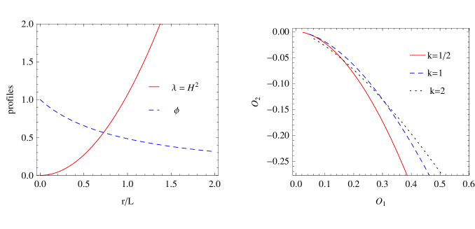
Figure 4: Left panel: profiles of the metric functions and the scalar field, in the extremal case, for a quartic potential with $k=1$ and $\gamma=-1$. Right panel: the function $O_{2}(O_{1})$ for three different values of $k$.

IV.2.2 Finite-temperature solutions

Using the same method described in Sect. IV.1.2 we have constructed, numerically, dressed BB solutions at finite temperature for models with the potential (42). We have generated global BB solutions for $m_{s}^{2}L^{2}=-2$ and for several values of the parameter $\Lambda$. These solutions interpolate between the near-horizon expansion (29) and the asymptotic AdS₄ form. In Fig. 5 we show an example of the metric and scalar profiles and the function $O_{2}(O_{1})$ for the case $m_{s}^{2}L^{2}=-2$ and for some selected values of $\Lambda$. As it is clear from Fig. 5, the function $O_{2}(O_{1})$ displays a universal linear behavior at small $O_{1}$, which already confirms that the boundary conditions are not conformal for any value of $\Lambda$. In addition, for larger values of $O_{1}$ the slope of $O_{2}(O_{1})$ depends on the quartic coupling.

In Fig. 6 we show the total mass of the solution as a function of the temperature for fixed horizon radius $r_{h}=1$ and $L=1$. As expected the dressed solutions exist only for $T>T_{0}$, confirming numerically the existence of the critical temperature $T_{0}$. It should be noticed that we have generated the numerical finite-temperature solutions for values of the parameters $m_{s}^{2}$ and $\Lambda$, which are different from those used to generate the extremal solutions. The reason for this choice is a numerical instability of the solutions for positive values of $m_{s}^{2}$.

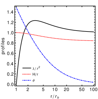
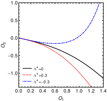
Figure 5: Left panel: metric and scalar profiles as functions of the (nonrescaled) coordinate $r$ for a quartic potential with $m^{2}_{s}L^{2}=-2$ and $\Lambda^{4}=0.3$. Right panel: the functions $O_{2}=O_{2}(O_{1})$ for different values of $\Lambda$.

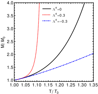
Figure 6: Total mass $M$ as a function of the temperature $T$ for a quartic potential and for selected values of the parameter $\Lambda$.

IV.3 Exponential potentials

In this section we will investigate the case of a theory with a potential $V(\phi)$ having the behavior described as type $b)$ in Section II, i.e. the potential behaves exponentially $\sim e^{b\phi}$ for $\phi\rightarrow\infty$ (corresponding to $r=0$).

We search for scalar-dressed BB solutions that smoothly interpolate between an asymptotic AdS spacetime and a near-horizon scale-covariant metric. In the dual QFT they correspond to a flow between an UV fixed point and hyperscaling violation in the IR. In general these interpolating solutions cannot be found analytically but have to be computed numerically. To be more concrete in the following we will focus on a class of models defined by the potential

$$V(\phi)=-\frac{2}{b^{2}L^{2}}[\cosh(b\phi)+3b^{2}-1].$$ (45)

This potential is such that the mass of the scalar is independent from the parameter $b$, $m_{s}^{2}=-2/L^{2}$. Moreover, it contains as particular cases $b=1/\sqrt{3}$, $b=1$ models emerging from string theory compactifications, for which analytical solutions are known Hertog and Maeda (2004); Cadoni et al. (2011).

IV.3.1 Extremal solutions

The leading near-horizon behavior of the extremal solutions can be captured by approximating the potential in the $\phi\rightarrow\infty$ region with the exponential form $V(\phi)=-(1/b^{2})e^{b\phi}$. In this case the field equations (3)-(5) give Cadoni et al. (2011)

$$\lambda = \alpha_{0}\left(\frac{r}{r_{-}}\right)^{w},\quad H=\left(\frac{r}{r_{-}}\right)^{w/2},\quad\phi=\phi_{0}-bw\ln\left(\frac{r}{r_{-}}\right),$$ (46)

$$\,\alpha_{0} = \frac{e^{b\phi_{0}}r_{-}^{2}}{b^{2}w(2w-1)},\quad w=\frac{2}{1+b^{2}}.$$

Notice that $\alpha_{0}>0$ requires $w>1/2$. This restricts the parameter range to $1/2<w<2$ ($0<b^{2}<3$). This ansatz provides an exact solution to the equations of motion with an exponential potential $-(1/b^{2})e^{b\phi}$ but only the leading near-horizon, extremal, behavior of the solutions with $V(\phi)$ generic. Solution (46) is scale covariant, i.e. the metric transforms under rescaling with a definite weight:

$$r\rightarrow kr,\quad(t,x,y)\rightarrow k^{1-w}(t,x,y),\quad ds^{2}\rightarrow k^{2-w}ds^{2}.$$ (47)

The extremal solution (46) contains an IR length-scale $r_{-}$. However, in the case of neutral BB the scaling transformations (47) may change this scale. The metric part of the solution is scale-covariant whereas the leading $\log r$ term of the scalar is left invariant. The only parameter that flows when IR length-scale $r_{-}$ is changed, is the constant mode $\phi_{0}$ of the scalar.

To reduce the number of independent parameters, we can exploit the symmetries of the field equations previously discussed [cf. Eqs. (III.1)] to fix $L=1$ and $\phi_{0}=0$ in Eq. (46). So we can start from the more simple ansatz containing only one free parameter $r_{-}$.

Starting from this scaling behavior near the horizon and imposing an AdS behavior (II) for the metric and the scalar field at infinity, we have integrated numerically the field equations with a potential given by Eq. (45), with different values of the parameter $0<b<\sqrt{3}$. We have found BB solutions with scalar hair, that interpolate between the near-horizon (46) and asymptotic (II) behavior.

In Fig. 7 we show the metric functions and the scalar field of these extremal BBs for $b=1/2$ and the function $P(O_{1})$ (obtained by varying the free parameter $r_{-}$) for different values of the parameter $b$. Also in this case we have checked numerically that $\lambda=H^{2}$  and that the conformal boundary conditions $P(O_{1})\sim O_{1}^{2}$ are satisfied. We have also explicitly checked that the mass of the extremal solution vanishes.

For the two cases $b=1/\sqrt{3}$ and $b=1$ the extremal solutions are known analytically Cadoni et al. (2011). They are respectively given by

$$\lambda = H^{2}=\frac{(r+r_{-})^{\frac{1}{2}}}{L^{2}}r^{\frac{3}{2}},\quad\phi=-\frac{\sqrt{3}}{2}\log\left(\frac{r}{r+r_{-}}\right),$$

$$\lambda = H^{2}=\frac{r+r_{-}}{L^{2}}r,\quad\phi=-\log\left(\frac{r}{r+r_{-}}\right),$$ (48)

where $r_{-}$ is a constant. From solutions (IV.3.1) one can easily derive the function $P(O_{1})$ defining the asymptotic boundary conditions for the scalar field. We have $P=(2/\sqrt{3})O_{1}^{2}$ for $b=1/\sqrt{3}$ and $P=O_{1}^{2}$ for $b=1$.

In order to compare these analytical solutions with those obtained numerically, we need to eliminate a linear term in the asymptotic behavior of $\lambda(r)$. Taking into account this translation, we have checked explicitly that our numerical solutions with $b=1/\sqrt{3}$ and $b=1$ and the numerical calculated functions $P$ exactly reproduce the analytical results. In general, the proportionality factor $f$ depends on the value of $b$. We observe that for $b<1$ $f$ is negative, for $b=1$ $f=0$, while for $b>1$ $f$ becomes positive, as shown in Fig. 7.

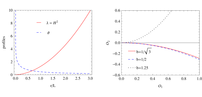
Figure 7: Left panel: profiles of the metric functions and the scalar field, in the extremal case, for the potential (45) with $b=1/2$ and $r_{-}=1$. Right panel: the function $O_{2}(O_{1})$ for three different values of $b$.

IV.3.2 Solutions at finite temperature

Following the same method as the one used in the previous subsections, one can generate generic hairy BB solutions with AdS asymptotics at finite temperature, i.e. solutions interpolating between the near-horizon (29) and the AdS (II) behavior. We have generated numerically these BB solutions and found, as in the case of quartic potential discussed above, that for every value of the parameter $b$ in the allowed range, they exist only for $r_{h}\geq 1$. This implies the existence of a critical temperature $T_{0}$ below which only the SAdS BB exists.

A summary of our results is presented in Fig. 8, which is qualitatively similar to Fig. 5 for the case of quartic scalar potential. Again we have verified that the function $O_{2}(O_{1})$ does not define conformal boundary conditions (9) for the scalar, i.e. the extremal solutions are isolated from those at finite temperature.

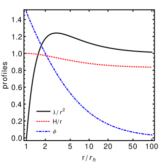
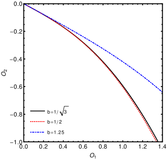
Figure 8: Left panel: metric and scalar profiles as functions of the (nonrescaled) coordinate $r$ for the potential (45) with $b=1/2$. Right panel: the functions $O_{2}=O_{2}(O_{1})$ for different values of $b$.

IV.4 Perturbative solutions near-extremality

In Sect. III.1 we have seen that the $T\rightarrow 0$ limit of finite-temperature BB solution is singular and that the ground state (26) is isolated from the continuous part of the spectrum. A way to gain information about the behavior near-extremality is to consider separately the near-horizon and near-extremal expansion. In general the two limits do not commute. In this section we will perform this perturbative analysis for the potential (45). Similar results can be obtained for other classes of potentials.

We look for perturbative solutions of the field equations (3)-(5) in the near-extremal, near-horizon regime. The near-extremal regime is obtained by expanding the metric functions $\lambda$ and $H$ and $\phi$ in power series of an extremality parameter $m$, with $m\rightarrow 0$ when the temperature $T\rightarrow 0$ (or the BB radius $r_{h}\rightarrow 0$). On the other hand the near-horizon regime is obtained by expanding the metric functions and the scalar field in power series of $r-r_{h}$. Because in general the two limits $m\rightarrow 0$ and $r\rightarrow r_{h}$ do not commute we have to consider separately the two cases.

IV.4.1 $r\to r_{h},\,r_{h}\to 0$

We first expand $\lambda$ and $H$ and $\phi$ in powers of $m$:

$$\lambda(r)=\sum_{n=0}^{\infty}\lambda_{n}(r)m^{n},\quad H(r)=\sum_{n=0}^{\infty}H_{n}(r)m^{n},\quad\phi(r)=\sum_{n=0}^{\infty}\phi_{n}(r)m^{n}.$$ (49)

For small BB radius $r_{h}<<L$ (or equivalently small $T$, i.e. $T<<1/L$) we can truncate in the perturbative expansion (49) to first order in $m$. At leading order we find that $\lambda_{0}$, $H_{0}$ and $\phi_{0}$ must satisfy the same field equations (3)-(5). At subleading order we find instead

$$H_{1}^{\prime\prime} = -\frac{1}{4}\left(2H_{0}\phi_{0}^{\prime}\phi_{1}+(\phi_{0}^{\prime})^{2}H_{1}\right),$$ (50)

$$\left(2\lambda_{0}H_{1}+H_{0}^{2}\lambda_{1}\right)^{\prime\prime} = 4\left[\lambda_{0}\left(H_{0}H_{1}\right)^{\prime}+\lambda_{1}H_{0}H_{0}^{\prime}\right]$$ (51)

$$\left(2\lambda_{0}H_{1}+H_{0}^{2}\lambda_{1}\right)^{\prime\prime} = -2\left(\phi_{1}H_{0}^{2}\frac{dV(\phi_{0})}{d\phi}+2H_{0}H_{1}V(\phi_{0})\right)$$ (52)

$$\left(\lambda_{0}H_{0}^{2}\phi_{1}^{\prime}+2\lambda_{0}H_{1}\phi_{0}^{\prime}+\lambda_{1}H_{0}^{2}\phi_{0}^{\prime}\right)^{\prime} = 2H_{0}H_{1}\frac{dV(\phi_{0})}{d\phi}+H_{0}^{2}\phi_{1}\frac{d^{2}V(\phi_{0})}{d\phi^{2}}$$ (53)

A solution of Eqs. (50)-(53) can be obtained by setting $\phi_{1}=H_{1}=0$, so that they reduce to

$$\left(H_{0}^{2}\lambda_{1}\right)^{\prime\prime}=0,\quad\left(H_{0}^{\prime}H_{0}\lambda_{1}\right)^{\prime}=0,\quad\left(H_{0}^{2}\phi_{0}^{\prime}\lambda_{1}\right)^{\prime}=0.$$ (54)

Equations (3)-(5) for the near-extremal leading order functions $\lambda_{0},H_{0},\phi_{0}$ can be now solved as a near-horizon expansion in powers of $r$. The leading term in this expansion being obviously given by Eq. (46),

$$\lambda_{0}(r) = \left(\frac{r}{r_{-}}\right)^{w}\sum_{n=0}^{\infty}\alpha_{n}\left(\frac{r}{r_{-}}\right)^{n},\quad H_{0}(r)=\left(\frac{r}{r_{-}}\right)^{\frac{w}{2}}\sum_{n=0}^{\infty}\beta_{n}\,\left(\frac{r}{r_{-}}\right)^{n},$$

$$\phi_{0}(r) = -bw\ln\frac{r}{r_{-}}+\sum_{n=0}^{\infty}\gamma_{n}\,\left(\frac{r}{r_{-}}\right)^{n}.$$ (55)

For each order in the $r$-expansion we can then determine the corresponding term $\lambda_{1}^{(n)}$ for $\lambda_{1}$ by solving Eqs. (54). One could worry about compatibility of the three equations (54). However, one can easily realize that for $H_{0}^{2}=c_{1}r^{l}$, the system (54) is always solved by $\lambda_{1}=c_{2}r^{-l+1}$ with $c_{1,2}$ constant. This follows from the first equation in (3), which implies $H_{0}^{\prime}\propto 1/r$. The leading order in the near-horizon expansion involves $w,\alpha_{0},\beta_{0},\gamma_{0}$. The symmetry of the field equations (3)-(5) under a rescaling of $H$ allows to fix $\beta_{0}=1$, whereas as expected $w,\alpha_{0}$ turn out to be given as in Eq. (46). At this order Eqs. (54) give in turn

$$\lambda_{1}^{(0)}\propto r^{-w+1}.$$ (56)

At the $n-$th order in the near-horizon expansion we find $\lambda_{1}^{(n)}\propto r^{-w-n+1}$. The form of the near-extremal solution is therefore given by,

$$\lambda=\lambda_{0}+\frac{m}{r^{w-1}}\left(\sum_{n=0}^{\infty}\frac{\epsilon_{n}}{r^{n}}\right)+\mathcal{O}(m^{2}),\quad H=H_{0},\quad\phi=\phi_{0},$$ (57)

where $\lambda_{0},H_{0},\phi_{0}$ are given by Eqs. (55). Assuming $m<0$ in the previous equation, we find that at leading order the relation between $m$ and $r_{h}$ is $m\propto r_{h}^{2w-1}$. Notice that this is an expansion in $1/r$. This means that terms with higher $n$ give smaller contributions for $r\rightarrow\infty$.

IV.4.2 $r_{h}\to 0$ , $r\to r_{h}$

This limit has been already discussed in section III.1. The expansion in powers of $(r-r_{h})$ is given by Eq. (29) and at leading order the field equations (3)-(5) give the relations (30) involving the parameters $a_{1,2},b_{0,1,2},c_{0,1}$. At the next to leading order we have three more parameters $a_{3},b_{3},c_{2}$ and three more relations. We are therefore left with 4 independent parameters $b_{0},c_{0},a_{1},r_{h}$. As previously discussed, the field equations have the symmetries (III.1) so that $r_{h}$ is the only independent parameter. In principle, one can now expand $a_{n}(r_{h}),b_{n}(r_{h}),c_{n}(r_{h})$ in powers of $r_{h}$, substitute in Eq. (29) and reorganize it as the power expansion in $m$ given by Eq. (49). By retaining only the linear terms in $m$ one could then compare the result with Eq. (57). Unfortunately, this is a very cumbersome task. Indeed, terms of order ${\mathcal{O}}(r_{h})$ are generated at any order in the near-horizon expansion (29). The problem has to be solved numerically. Numerically, one can look for global solutions interpolating between the near-horizon behavior (29) with a given $r_{h}$ and the AdS asymptotic solution (II). There is no guarantee that the solutions obtained in this way match Eq. (57). This is because the two limits $r\rightarrow r_{h}$ and $r_{h}\rightarrow 0$ do not commute.

IV.4.3 Near-extremal numerical solutions

We have generated numerically, for the case of the potential (45), the solutions interpolating between the AdS asymptotic behavior (II) and the near-extremal regime given by Eq.(57). In Fig. 9 (left panel) we can see the profiles of the metric functions and the scalar field for $b=1/\sqrt{3}$ and $r_{h}=10^{-2}$ (corresponding to $m=-10^{-4}$).

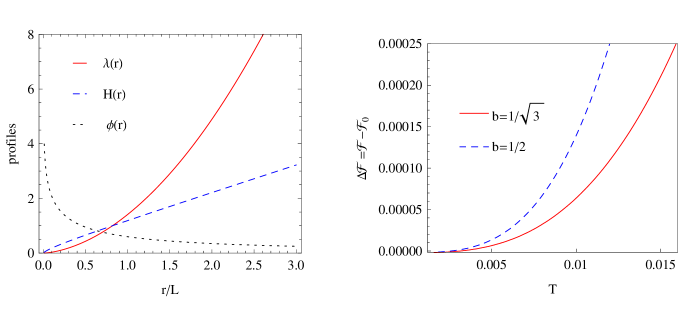
Figure 9: Left panel: interpolating solutions between AdS at infinity and the near-extreme regime given by Eq. (57) with $b=1/\sqrt{3}$ and $r_{h}=10^{-2}$. Right panel: difference between the free energy density of the near-extremal BB solution and the free energy density of the $SAdS$ BB, for two values of $b$.

We see that although the $T\to 0$ limit of the near-horizon perturbation theory is singular and isolated, global solutions obtained interpolating the near-horizon, near-extremal behavior (57) with AdS₄ exist also for $T>0$. This is a manifestation of the noncommutativity of the near-horizon and near extremal limit. From the point of view of perturbation theory, the $T=0$ singularity means that the perturbative series in $m$ (49) do not converge and that solutions (57) are only perturbative solutions valid for $r_{h}<<L$.

The hairy near-extremal solutions shown in Fig. 9 describe small thermal perturbations of the extremal solution, but they do not describe the small-$T$ limit of finite-temperature solutions. These results confirm that the ground state solutions (26) are not smoothly connected to the finite-$T$ solutions, because of the existence of the discontinuity.

Perturbative solutions in the small scalar-field limit can be also constructed. These kind of solutions are described in the Appendix.

IV.5 Hyperscaling violation and critical exponents

The extremal $T=0$ hairy solutions found in Sect. IV.3 for the case of the potential (45) describe a flow between the near-horizon regime (IR) hyperscaling violating regime and an asymptotic AdS fixed point. From a QFT point of view, this translates into a hyperscaling-violation phase in the IR and a scaling-preserving phase in the UV. We can characterize the holographic features of this flow by giving the scaling exponents in the conformal (AdS) phase and nonconformal (hyperscaling violating) phase. The IR behavior is dictated by Eqs. (46). The UV metric is instead that of AdS₄.

To describe hyperscaling violation in four dimensions it is useful to consider the following parametrization of the scale covariant metric:

$$ds^{2}=r^{\theta-2}(-r^{-2(z-1)}dt^{2}+dx_{i}^{2}+dr^{2}),$$ (58)

where $\theta$ is the hyperscaling violation parameter and $z$ the dynamic critical exponent. Under the following rescaling of the coordinates:

$$t\rightarrow\lambda^{z}t,\text{ \ \ }x_{i}\rightarrow\lambda x_{i},\text{ \ \ }r\rightarrow\lambda r,\text{ }$$

the metric (58) transforms as:

$$\text{\ \ }ds\rightarrow\lambda^{\theta/2}ds.$$

Moreover, this scaling transformation determines the following scaling behavior for the free energy:

$$F\sim T^{\frac{2-\theta+z}{z}}.$$ (59)

By a simple redefinition of the radial coordinate and a rescaling of the coordinates, we can write the metric (46) in the form (58). We obtain:

$$ds^{2}=r^{\frac{w}{1-w}}(-dt^{2}+dx_{i}^{2}+dr^{2}).$$ (60)

Comparing Eq. (60) with Eq. (58), we can easily extract the parameters $\theta$ and $z$ of our solution:

$$z=1,\text{ \ \ }\theta=\frac{2-w}{1-w}.$$ (61)

Notice that we are now using dimensionless coordinates $r,t,x_{i}$, so that the IR length-scale $r_{-}$ drops out from the solution. While the value $z=1$ of the dynamic critical exponent is largely expected for uncharged solutions, we see that $\theta\leq 0$ for $1<w\leq 2$ and $\theta>2$ for $1/2<w<1$, while $\theta$ diverges for $w=1$ (recall that in our case $1/2<w\leq 2$). This is in agreement with the null energy conditions for the stress-energy tensor, which require, for $z=1$ and in the general case of $d+2$ dimensions, either $\theta\leq 0$ or $\theta\geq d$. Trivially, the parameters of the UV AdS conformally invariant solution are $z=1,\text{\ }\theta=0$.

From Eq. (59), substituting the (61), we get that the free energy scales as:

$$F\sim T^{\frac{1-2w}{1-w}}.$$ (62)

We see from Eq. (62) that the exponent of $T$ is negative for $0<w<1$ or, equivalently, when $\theta>2$. So in this case the free energy diverges for $T\rightarrow 0$ and the corresponding phase is always unstable.

IV.6 Thermodynamics of the near-extremal solutions

The hairy near-extremal solutions discussed above can be interpreted as small thermal fluctuations of extremal $T=0$ hairy BBs. The thermodynamical features of these BB solutions – in particular the free energy and the specific heat – will provide important information about the stability of the ground state. Properties such as the scaling exponents are determined by the behavior of the system at the quantum critical point, namely by the $T=0$ scale-covariant extremal near-horizon solution (46). On the other hand the stability properties are global features and they must be investigated using the global $T\neq 0$ solutions.

By Eqs. (14), the temperature and the entropy density of the near-horizon, near-extremal solution (57) are given at leading order by:

$$T=\frac{2w-1}{4\pi}\alpha_{0}r_{h}^{w-1},\quad{\mathcal{S}}=\frac{(4\pi)^{\frac{2w-1}{w-1}}}{[\alpha_{0}(2w-1)]^{\frac{w}{w-1}}}T^{\frac{w}{w-1}}.$$ (63)

Notice that in these subsections we are using dimensionless coordinates, so that the IR length-scale $r_{-}$ drops out from our formulae, as in Eq. (60), and we set $L=1$. Temperature and entropy density are therefore also dimensionless.

The scaling exponent of the entropy becomes negative when $1/2<w<1$ (corresponding to $1<b^{2}<3$), implying a negative specific heat and the corresponding solutions are therefore unstable. This is in agreement with the results of the previous subsection concerning the scaling of the free energy for $w<1$. Moreover, in this case small values of the temperature correspond to high values of the horizon $r_{h}$ and of the parameter $m$, so that we cannot obtain near-extremal solutions (in the sense of small temperature solutions) with $r_{h}<<1$, which is the range of validity of the perturbative solutions (57).

For what concerns the entropy density and free energy density $\mathcal{F}_{0}$ of the SAdS BB we have

$$\mathcal{S}_{0}=\frac{\left(4\pi\right)^{3}}{9}T^{2},\quad\mathcal{F}_{0}=-\left(\frac{4\pi}{3}\right)^{3}T^{3}.$$

We have derived numerically the free energy of the numerical near-extremal solutions as a function of the temperature, for $T<<1$ . In Fig. 9 (right panel) we show the behavior of the free energy density of the hairy BB solution compared with the free energy density of the SAdS BB for two selected values of the parameter $b$ (both such that $1<w<2$), and for small values $T<<1$ of the temperature. We observe that the scalar-dressed solutions are energetically disfavored against the SAdS BB. This result can also be verified analytically by comparing $\mathcal{F}$₀ with the free energy density $\mathcal{F}$ of the hairy near-extremal solution, which can be expressed as a function of the temperature using Eq. (14).

IV.7 Thermodynamics of the finite temperature solutions

We have also computed the free-energy $F$ and the specific heat $c$ of the finite-temperature numerical scalar-dressed solutions derived in the previous sections for the case of the quartic (42) and exponential (45) potential. The results are shown in Fig. 10 where we plot $\Delta F/F_{0}$ and $c$ as a function of the temperature, with $\Delta F=F-F_{0}$. The free energy $F$ is always larger than that of the corresponding Schwarzschild-AdS BB at same temperature and the specific heat is negative. Hence, these solutions are energetically disfavored against the undressed ones.

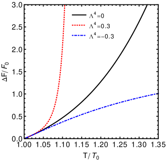
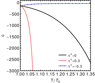
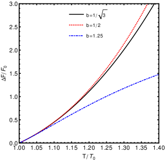
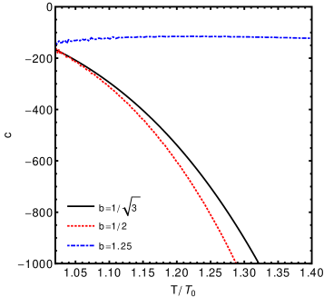
Figure 10: Free energy (left panels) and specific heat (right panels) of the dressed BBs as a function of the temperature. Top and bottom panels refer to the theory with a quartic potential with $m_{s}^{2}=-2$ and with the exponential potential (45), respectively.

V Charged solutions

In this section, we will extend the numerical results previously obtained for neutral BBs in ES-AdS gravity to the case of finite charge density, i.e to the case in which an EM field is present in the bulk. We will focus our attention on models with exponential (45) or quadratic (11) potential. We will discuss separately the cases of: i) minimal gauge coupling $Z=1$; ii) exponential gauge coupling in the $U(1)-$symmetry preserving phase; iii) Minimal gauge coupling in the $U(1)-$symmetry breaking phase ($Z=1,\,Y\neq 0$).

V.1 Minimal gauge coupling

In this section we will construct numerical BB solutions for the model (1) with $Z=1,Y=0$ and the potential (45). As usual we discuss separately extremal and finite temperature solutions.

V.1.1 Extremal solutions

Following the same approach as the one used for the case of electrically neutral solutions, we look for numerical scalar-dressed BB’s solutions interpolating between an asymptotic AdS spacetime and a near-horizon scale-covariant metric. Also in this case, the near-horizon behavior can be captured by approximating the potential (45) in the $\phi\rightarrow\infty$ region with the exponential form $V(\phi)=-(1/b^{2})e^{b\phi}$. The field equations (3) – (5) give the scale covariant solution, which in the dual QFT corresponds to hyperscaling violation:

$$\lambda = \alpha_{0}\left(\frac{r}{r_{-}}\right)^{w},\quad H=\left(\frac{r}{r_{-}}\right)^{h},\quad\phi=\phi_{0}-\frac{b}{4}(w+2)\ln\left(\frac{r}{r_{-}}\right),\text{ \ \ }$$ (64)

$$w = 2-4h=\frac{8-2b^{2}}{4+b^{2}},$$

$$\,\alpha_{0} = \frac{8e^{b\phi_{0}}r_{-}^{2}}{b^{2}w(w+2)},\quad\rho^{2}=\frac{2e^{b\phi_{0}}(3w-2)}{b^{2}(w+2)},$$

where $\rho$ is the charge density of the solution. The solution above, together with the condition $\alpha_{0}>0$, restricts the parameter range to $2/3<w<2$ (corresponding to $0<b^{2}<2$). We can exploit the symmetries of the field equations to fix $L=1$ and $\phi_{0}=0$, leaving $r_{-}$ the only free parameter. We immediately note an important feature of this solution: in the limit $\rho\rightarrow 0$ it does not reduce to the near-horizon solution (46) obtained in the electrically neutral case. This means that the uncharged solution (46) and the electrically charged solutions (64) represent two disjoint classes of solutions.

As usual, starting from this near-horizon scaling and imposing an AdS behavior (II) at infinity, we have integrated numerically the field equations for different values of the parameter $b$, finding numerical solutions only for $b>1/2$. In Fig. 11 we show the fields for $b=1$. As expected, here we find in general $\lambda\neq H^{2}$, hence the mass of the solution is nonvanishing and the degeneracy with the AdS vacuum is removed.

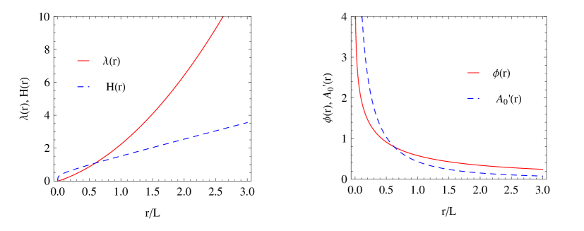
Figure 11: Metric functions (left panel) and scalar and Maxwell field (right panel), in the extremal case, for the potential (45) with $b=1$ and $r_{-}=1$.

V.1.2 Finite-temperature solutions

At variance with the extremal case, the charge of finite temperature solutions is a free parameter and the uncharged case is obtained setting $\rho=0$. Using a straightforward extension of the numerical integration previously discussed, we can construct finite-temperature solutions at fixed charge density $\rho$. Some examples are shown in Fig. 12 for the potential (45) with $b=1$. In the left panel we show the radial profiles of the fields, in the central panel we show the function $O_{2}=O_{2}(O_{1})$ for different values of $\rho$, and in the right panel we shown the difference between the free energy of the dressed solution and that of a RN BB with same radius and same charge. Notice that, as already stressed, in the charged case the boundary conditions can be arbitrarily chosen. In particular, one can also choose conformal boundary conditions of the form $O_{1}=0$. However, in the case at hand we have found that such conditions do not allow for scalar-dressed BBs.

Similarly to the uncharged case, these dressed solutions are always energetically disfavored with respect to the undressed ones.

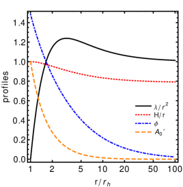
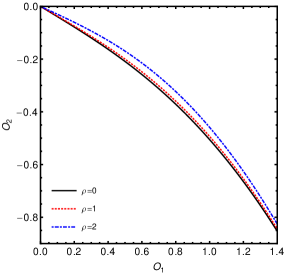
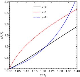
Figure 12: Left panel: profiles for the metric coefficients, scalar field and EM potential as functions of the (nonrescaled) coordinate $r$ for the potential (45) with $b=1$ and different values of $\rho$. Central panel: the functions $O_{2}=O_{2}(O_{1})$ for different values of $\rho$ and $b=1$. Right panel: difference between the free energy of the dressed solution and that of a RN BB with same radius and same charge.

V.2 Nonminimal gauge coupling

As an example of a model with nonminimal gauge coupling we consider here the model discussed in Ref. Cadoni et al. (2010). The gauge coupling $Z$ and the potential $V$ are Cadoni et al. (2010)

$$Z(\phi)=2Z_{0}\cosh a\phi,\text{ \ \ \ \ \ }\,V(\phi)=-2V_{0}\cosh b\phi.$$ (65)

In the IR ($\phi\rightarrow\infty$) both the gauge coupling $Z$ and the potential $V$ behave exponentially. The model therefore belongs to the wide class of EHTs that flow to a hyperscaling violating phase in the IR Charmousis et al. (2009); Cadoni et al. (2010); Goldstein et al. (2010a); Dong et al. (2012); Gouteraux and Kiritsis (2012). The extremal solution of the field equations in the near-horizon approximation is the scale-covariant metric Cadoni et al. (2010):

$$\lambda = \alpha_{0}\left(\frac{r}{r_{-}}\right)^{w},\quad H=\left(\frac{r}{r_{-}}\right)^{h},\quad\phi=\phi_{0}-\xi\ln\left(\frac{r}{r_{-}}\right),\text{ \ \ }$$ (66)

$$\xi = \frac{4(a+b)}{4+(a+b)^{2}},\text{ \ \ }w=2-4ch,\text{ \ \ \ \ }c=\frac{b}{a+b},$$

$$\,\alpha_{0} = \frac{2V_{0}e^{b\phi_{0}}r_{-}^{2}}{(w+2h)(w+2h-1)},\quad\frac{\rho^{2}}{Z_{0}}e^{-a\phi_{0}}=\frac{2V_{0}e^{b\phi_{0}}(2-2h-b\xi)}{(w+2h)}.$$

In Ref. Cadoni et al. (2010) $T=0$ global solutions interpolating between the near-horizon hyperscaling violating metric (66) and the asymptotic AdS₄ geometry have been constructed numerically. Furthermore, numerical finite-temperature solutions have been found and their properties have been discussed in detail. In particular, it has been shown that below a critical temperature $T_{c}$ the system undergoes a phase transition. The scalar dressed BB solution becomes energetically preferred with respect to the RN BB.

The results of Ref. Cadoni et al. (2010) fully confirm the general results of Sect. III. The finite charge density removes the degeneracy of the $T=0$ solution we have in the uncharged case. Comparing the charged solution (66) with the neutral solution (46) one easily realizes that although the IR behavior of the two solutions belongs to the same class (hyperscaling violating) the critical exponents change. Moreover, the nonminimal coupling between the scalar field and the Maxwell field is such that the energy of the extremal scalar-dressed solution is smaller than that of the RN-solution. This determines an IR quantum phase transition between the AdS${}_{2}\times R^{2}$ near-horizon geometry of the RN BB and the near-horizon scale covariant geometry (66). In the dual QFT this corresponds to a phase transition between a conformal and a hyperscaling violating fractionalized phase.

Because the thermodynamical properties of the system at small temperature are essentially determined by the $T=0$ quantum phase transition, this also explains why the hyperscaling violating phase is stable at small temperature, below $T_{c}$.

The near-horizon solutions for the charged BB (64) and (66) depend on the same IR length-scale $r_{-}$ as the neutral BB solution (46). However, in the charged case the scaling transformations under which the metric part of the solutions is scale-covariant, changes not only the constant mode of the scalar $\phi_{0}$ but also the charge density $\rho$. Thus, changing the IR scale $r_{-}$ corresponds to a flow of the charge density $\rho$. As noticed already in Ref. Gouteraux and Kiritsis (2012), this is an irrelevant deformation along the hyperscaling violating critical line.

It is also interesting to notice the different role played in the quantum phase transition by the finite charge density and the nonminimal gauge coupling. The finite charge density lifts the degeneracy of the $T=0$ vacuum and changes the values of the critical exponents of the hyperscaling violating solution, but it is by itself not enough to make the hyperscaling violating phase energetically competitive with respect to the conformal AdS${}_{2}\times R^{2}$ phase. Indeed, in the case of minimal gauge couplings discussed in the previous subsection, the energy of extremal RN-BBs is lesser than the energy of the scalar-dressed $T=0$ solution. It is the non minimal coupling between the gauge and the scalar field that makes the extremal RN solution energetically disfavored with respect to the extremal scalar-dressed solution.

V.2.1 Hyperscaling violation and critical exponents

In the case of a potential behaving exponentially in the IR the near-horizon, extremal solutions are scale-covariant for both zero or finite charge density and for both minimal or nonminimal gauge couplings. On the other hand, the critical exponents are affected by switching on a finite charge density. In particular in the case of charged solutions we will always have $z\neq 1$.

In the minimal case, after a redefinition of the radial coordinate and a rescaling of the coordinates, the metric (64) reads:

$$ds^{2}=r^{2}\left(-r^{\frac{2(3w-2)}{2-w}}dt^{2}+dr^{2}+dx_{i}^{2}\right),$$

from which we can easily extract the critical parameters:

$$\theta=4,\text{ \ }z=\frac{2(2-2w)}{2-w}.$$

We note immediately that the hyperscaling violation exponent $\theta$ is a (positive) constant, independent from the parameters of the potential. The range of $w$ implies $z<1$, which is in agreement with the NEC conditions. Indeed the latter impose, for this values of $\theta$ and $z$, the conditions $z>2$ or $z<1$. Moreover we note that for $1<w<2,$ $z$ is negative.

On the other hand, for $2/3<w<1$ (corresponding to $0<z<1$), the free energy scales with a negative exponent:

$$F\sim T^{\frac{2-\theta+z}{z}}=T^{\frac{w}{2w-2}},$$

which implies an instability of the corresponding phase and a negative specific heat.

Finally, we consider the case of a nonminimal gauge coupling given by Eq. (65). The critical exponents can be read off from Eq. (66), after a reparametrization of the radial coordinate which puts the metric in the form (60). We have

$$\theta=\frac{4c}{2c-1}\ \ ,\ \ z=\frac{2c(2-2w)}{(2c-1)(2-w)},$$

while the free energy scales as:

$$F\sim T^{\frac{2-\theta+z}{z}}=T^{\frac{(2c-1)w+2-2c}{c(2w-2)}}.$$ (67)

V.3 Symmetry-breaking phase

As an example of a model having a $U(1)$-symmetry-breaking phase we consider here the model discussed in Ref. Hartnoll et al. (2008a, b); Horowitz and Roberts (2008, 2009), which gives the simplest realization of holographic superconductors. The gauge coupling is minimal, while the potential $V$ and the function $Y(\phi)$ in the action (1) are quadratic Horowitz and Roberts (2009):

$$Z(\phi)=1,\,\text{\ \ \ \ \ }V(\phi)=\frac{m_{s}^{2}}{2}\phi^{2},\,\ \ \ \ \ Y(\phi)=q^{2}\phi^{2},$$

where $q$ is the electric charge of the complex scalar field whose modulus is $\phi$.

The metric and scalar field associated to the $T=0$ solution of the field equations in the near-horizon approximation are given as in the neutral case discussed in Sect. IV.1, i.e. by Eq. (40), whereas the EM potential is $A_{0}=\phi_{0}\hat{r}^{\beta}(-\log\hat{r})^{1/2}$ with $2\beta=-1\pm(1-48q^{2}/m_{s}^{2})^{1/2}$. Numerical, extremal solutions interpolating between the near-horizon solution (40) and AdS₄ have been constructed for $q^{2}>|m^{2}_{s}|/6$ in Ref. Horowitz and Roberts (2009). Numerical finite-temperature solutions have been also considered Hartnoll et al. (2008a, b); Horowitz and Roberts (2008). In particular, it is well known that below a critical temperature the superconducting phase (corresponding in the bulk to the scalar-dressed BB solution) becomes energetically preferred.

The results of Ref. Hartnoll et al. (2008a, b); Horowitz and Roberts (2008, 2009) for the holographic superconductors fully confirm our general results of Sect. III. The finite charge density removes the degeneracy of the $T=0$ solution in the uncharged case. Moreover, the nonvanishing coupling function $Y$ gives a mass to the $U(1)$ gauge field and makes the extremal scalar-dressed solution energetically competitive with respect to the RN-solution. The system represents an IR quantum phase transition between the AdS${}_{2}\times R^{2}$ near-horizon geometry of the RN BB and the near-horizon geometry (40). In the dual QFT this corresponds to the superconducting phase transition Hartnoll et al. (2008a, b); Horowitz and Roberts (2008, 2009), which occurs below the critical temperature.

Similarly to the nonminimal case, also here the finite charge density and the nonvanishing function $Y$ play a very different role. The finite charge density simply lifts the degeneracy of the $T=0$ vacuum we have in the uncharged case. But it is the coupling between the scalar field and the EM potential $A_{0}$ that causes the superconducting phase transition to occur at the critical temperature. It is also interesting to notice that in this case the finite charge density does not change the metric (and scalar) part of the IR solution, which is determined by the near-horizon solution and it is described as in the EM neutral case by Eq. (40).

VI Concluding remarks

In this paper we have discovered several interesting features of scalar condensates in EHTs, which may be relevant for understanding holographic quantum phase transitions. In particular, we have shown that for zero charge density the ground state for scalar-dressed, asymptotically AdS, BBs must be degenerate with the AdS vacuum, must be isolated from the finite-temperature branch of the spectrum and must satisfy conformal boundary conditions for the scalar field. This degeneracy is the consequence of a cancellation between a gravitational positive contribution to the energy and a negative contribution due to the scalar condensate. When the scalar BB is sourced by a pure scalar field with a potential behaving exponentially in the IR, a scale is generated in the IR.

Switching on a finite charge density $\rho$ for the scalar BB, the degeneracy of the ground state is removed, the ground state is not anymore isolated from the continuous part of the spectrum and the flow of the IR scale typical of hyperscaling violating geometries determines a flow of $\rho$. Depending on the gauge coupling between the bulk scalar and EM fields, the new ground state may be or may not be energetically preferred with respect to the extremal RN-AdS BB. We have also explicitly checked these features in the case of several charged and uncharged scalar BB solutions in theories with minimal, nonminimal and covariant gauge couplings. In the following subsections we will briefly discuss the consequences our results have for the dual QFT and for quantum phase transitions.

VI.1 Dual QFT

One striking feature of the uncharged scalar BB solutions we discussed is that the boundary conditions for the scalar field are either determined by the symmetries (for the ground state) or by the dynamics (for finite-temperature solutions). Because the only free function entering the model is the scalar potential $V(\phi)$, this means that the information about boundary conditions for the scalar field is entirely encoded in the symmetries of the field equations and in $V$. Since the scalar field drives the holographic renormalization group flow, this fact has some interesting consequence for the dual QFT.

We have seen in Sect. III that in the case of zero charge density the ground state for the scalar BB must be characterized by conformal boundary conditions. From the point of view of the dual QFT this corresponds to a multi-trace deformation of the Lagrangian of the CFT. This is a relevant deformation, associated to a relevant operator, which will produce a renormalization-group flow from an UV CFT to an IR QFT. The nature of the IR QFT is entirely determined by the self-interaction potential, $V(\phi)$. In the case of the quartic potential (42) – which is characterized by two extrema – the IR QFT has the form of a further CFT. In the case of the exponential potential (12) the IR QFT is characterized by hyperscaling violation. In the case of the quadratic potential (11) the characterization of the IR QFT is much less clear because of the absence of scaling symmetries.

The characterization of the dual QFT at finite temperature is much more involved. In this case we have generically nonconformal boundary conditions for the scalar field and the asymptotic AdS isometries are broken. Nonetheless, an asymptotic time-like killing vector exists and both the UV and the IR QFT should admit a description in terms of multi-trace deformations of a CFT.

On the other hand we have shown that the ground state and finite$-T$ states are not continuously connected. This means that we are dealing here with two different disjoint sets of theories.

This picture changes completely when one adds a finite charge density. Now the boundary conditions for the scalar field can be arbitrarily chosen, for instance in the form of the usual conformal Neumann or Dirichlet boundary conditions. Thus, in the case of finite charge, we have the usual description borrowed from the AdS/CFT correspondence with single trace operators dual to the scalar field.

VI.2 Scalar condensate and quantum criticality

The results of this paper improve our understanding of quantum critical points in EHTs. In particular they shed light on the phase structure of these critical points proposed in Ref. Gouteraux and Kiritsis (2012) and on their stability.

The degeneracy of the ground state for uncharged BBs simply means that at zero charge density the hyperscaling violating critical point (or line) and the hyperscaling-preserving critical point have the same energy. The potential $V$ for the scalar field determines completely the scaling symmetry and the critical exponents of the hyperscaling violating critical point. The renormalization group flow from the UV conformal fixed point into the IR introduces an emergent IR scale. Changing this IR scale produces a flow of the constant mode of the scalar field. As already noted in Ref. Gouteraux and Kiritsis (2012), the presence of this arbitrary scale implies that hyperscaling violating critical points appear as critical lines rather than critical points. On the other hand, for scalar-dressed BBs the ground state is isolated from the finite$-T$ part of the spectrum and the states at finite temperature are always energetically disfavored with respect to the SAdS BB. Thus, at zero charge density there is no phase transition between the hyperscaling preserving phase and the hyperscaling violating phase.

Considering charged scalar BBs, i.e. introducing a finite charge density $\rho$ in the dual QFT, generates several effects. First of all the degeneracy of the ground state is lifted and the ground state is not anymore isolated from the $T>0$ continuous branch of the spectrum. The change of the IR scale typical of hyperscaling violating critical lines now also produces a flow of the charge density $\rho$. Although the critical exponents are modified by the presence of a finite charge density (for instance the dynamical critical exponent $z$ becomes $\neq 1$) the scaling symmetries characterizing the critical point are very similar to those we have in the case of $\rho=0$. The similarity between the ground state geometries in the $\rho\neq 0$ and $\rho=0$ case is even more striking in the case of covariant gauge coupling (the case of holographic superconductors). In this latter case the metric and scalar part of the near-horizon solution is exactly the same for $\rho\neq 0$ and $\rho=0$.

The stability of the hyperscaling violating critical line is a far more involved question. It turns out that it depends crucially on the coupling between the scalar condensate and the EM field, i.e. on the two coupling functions $Z(\phi)$ and $Y(\phi)$ in the action (1). In all cases that we have considered with a minimal gauge coupling $Z=1$, and in absence of $U(1)$ symmetry breaking ($Y=0$), the hyperscaling preserving phase is always energetically preferred with respect to the hyperscaling violating one. In this case, an IR phase transition between hyperscaling-preserving phase and the hyperscaling violating phase does not occur.

Conversely, in the two cases of a nonminimal gauge coupling behaving exponentially in the IR ($Z\sim e^{a\phi}$, $Y=0$) and covariant gauge coupling ($Z=1,\,Y\sim\phi^{2}$), the hyperscaling violating phase is energetically preferred. This gives, respectively, the IR phase transitions between the hyperscaling preserving phase and the hyperscaling violating phase found in Ref. Cadoni et al. (2010) and the well-known superconducting phase transition of Ref. Hartnoll et al. (2008a, b); Horowitz and Roberts (2008, 2009). On the other hand, considering charged BBs at finite temperature, the critical temperature of the phase transition between the hyperscaling-preserving/hyperscaling violating phases is settled by the charge density $\rho$ Cadoni et al. (2010), i.e by the IR emergent scale typical of the hyperscaling violating critical line.

Summarizing, our results strongly indicate that for EHTs described by (1) the three coupling functions $V(\phi),\,Z(\phi),\,Y(\phi)$ determine different features of holographic quantum critical points. The self-interaction potential $V(\phi)$ determines the scaling symmetries but not the stability of hyperscaling violating phases. Conversely $Z$ and $Y$ are crucial in determining the stability, the breaking of the $U(1)$ symmetry and the characterization as fractionalized or cohesive of the hyperscaling violating phase.

Appendix A Uncharged perturbative solutions in the small scalar-field limit

In the neutral case, it is possible to construct analytical BB solutions in the small scalar-field limit perturbatively, i.e. expanding the solution as follows

$$\lambda(r) = \frac{r^{2}}{L^{2}}-\frac{M}{2r}+\epsilon^{2}\lambda_{2}(r)\,,$$ (68)

$$H(r) = r+\epsilon^{2}H_{2}(r)\,,$$ (69)

$$\phi(r) = \epsilon\phi_{1}(r)\,.$$ (70)

where $\epsilon$ is a book-keeping parameter of the expansion. The solution for the scalar field can be obtained by solving the scalar equation at first order. The regular solution, can then be inserted into the Einstein equations that, to second order, can be solved for $\lambda_{2}$ and $H_{2}$.

Let us start with the $T=0$ AdS₄ vacuum, i.e. we set $M=0$ in the equations above. To second order in the scalar field, the solution reads

$$\lambda(r) = \frac{r^{2}}{L^{2}}+\left(-\frac{O_{1}^{2}}{4L^{2}}-\frac{O_{2}^{2}}{6L^{2}r^{2}}+\frac{2rC_{1}}{L^{2}}+\frac{C_{2}}{r}\right)\epsilon^{2}+\mathcal{O}(\epsilon^{4})\,,$$ (71)

$$H(r) = r+\left(-\frac{O_{2}^{2}}{12r^{3}}-\frac{O_{1}O_{2}}{6r^{2}}-\frac{O_{1}^{2}}{8r}+C_{1}+rC_{2}\right)\epsilon^{2}+\mathcal{O}(\epsilon^{4})\,,$$ (72)

$$\phi(r) = \epsilon\left(\frac{O_{1}}{r}+\frac{O_{2}}{r^{2}}\right)+\mathcal{O}(\epsilon^{3})\,,$$ (73)

where $C_{i}$ are integration constants. This is a solution for the classes of potentials presented in the main text. Although not presented, the solutions can be obtained in closed form at least to fourth order. The constant $C_{1}$ can be set to zero by performing a coordinate translation such that the asymptotic form of the metric reads as in Eq. (III.1) with $C_{2}=-m_{0}/2$ being related to the metric contribution to the gravitational mass and after a rescaling $H\to H/(1+\epsilon^{2}C_{2})$, which can be performed by rescaling the the transverse coordinates. Interestingly, there exists an event horizon, so the solution represents a BB endowed with a scalar field. Let us consider two cases separately: $O_{2}=0$ and $O_{2}=O_{2}(O_{1})$ (without loss of generality, we assume $O_{2}\geq 0$). For the latter case, the horizon is located at

$$r_{h}=\frac{\sqrt{O_{2}}\epsilon}{6^{1/4}}+\frac{\sqrt{3}m_{0}}{4\sqrt{2}O_{2}}\epsilon+\frac{3^{1/4}\left(4O_{1}^{2}O_{2}^{2}-3m_{0}^{2}\right)}{2^{3/4}32O_{2}^{5/2}}\epsilon^{3/2}+\mathcal{O}(\epsilon^{5/2})\,,$$ (74)

and, to first order, the temperature of the solution is

$$T=\frac{\sqrt{O_{2}}\sqrt{\epsilon}}{6^{1/4}\pi}\,.$$ (75)

On the other hand, if $O_{2}=0$, the horizon and the temperature read

$$r_{h} = \frac{m_{0}^{1/3}\epsilon^{2/3}}{2^{1/3}}+\frac{O_{1}^{2}\epsilon^{4/3}}{2^{2/3}6m_{0}^{1/3}}\,,$$ (76)

$$T = \frac{3m_{0}^{1/3}\epsilon^{2/3}}{2^{1/3}4\pi}+\frac{O_{1}^{4}\epsilon^{2}}{96m_{0}\pi}$$ (77)

In general, these solutions describe a BB whose horizon shrinks to zero in the $\mathcal{O}_{i}\to 0$ limit. The total mass of the BB is given by Eq. (15) and it coincides with $m_{0}$ when $O_{2}=0$. It is interesting to compare the free energy of this solution with that of a SAdS BB at the same temperature. When $O_{2}\neq 0$, we obtain

$$F-F_{0}=\frac{37(\epsilon O_{2})^{3/2}}{6^{3/4}27}+\mathcal{O}(\epsilon^{2})\,,$$ (78)

so that $F>F_{0}$ for any $O_{2}\neq 0$ and the dressed solution is always energetically disfavored. Note that this result is valid for any boundary condition $O_{2}=O_{2}(O_{1})\neq 0$ and for any scalar potential whose expansion reads $V\sim-6/L^{2}-\phi^{2}/L^{2}$. On the other hand, if $O_{2}=0$, $F=F_{0}$ to second order in $O_{1}$, so that the two solutions are degenerate.

Finally, we can adopt the same technique to construct perturbative solutions of the SAdS BB at finite temperature. At first order, the general solution of the scalar field equation reads

$$\phi_{1}=\alpha P_{-1/3}\left[{r^{3}}/(L^{2}M)-1\right]+\beta Q_{-1/3}\left[{r^{3}}/(L^{2}M)-1\right]\,,$$ (79)

where $P_{n}$ and $Q_{n}$ are Legendre functions of order $n$ and $\alpha$ and $\beta$ are integration constants. Imposing regularity at the horizon $r_{h}=(2L^{2}M)^{1/3}$ requires $\beta=0$. In principle, this solution can be inserted in the Einstein equation in order to obtain two equations for $H_{2}(r)$ and $\lambda_{2}(r)$. Unfortunately, these equations do not appear to be solved in closed form.

References

- Hartnoll et al. (2008a) S. A. Hartnoll, C. P. Herzog, and G. T. Horowitz, Phys. Rev. Lett. 101, 031601 (2008a), eprint 0803.3295.
- Hartnoll et al. (2008b) S. A. Hartnoll, C. P. Herzog, and G. T. Horowitz, JHEP 12, 015 (2008b), eprint 0810.1563.
- Horowitz and Roberts (2008) G. T. Horowitz and M. M. Roberts, Phys.Rev. D78, 126008 (2008), eprint arXiv:0810.1077.
- Herzog (2009) C. P. Herzog, J. Phys. A42, 343001 (2009), eprint 0904.1975.
- Hartnoll (2009) S. A. Hartnoll, Class. Quant. Grav. 26, 224002 (2009), eprint 0903.3246.
- Charmousis et al. (2009) C. Charmousis, B. Gouteraux, and J. Soda, Phys. Rev. D80, 024028 (2009), eprint 0905.3337.
- Cadoni et al. (2010) M. Cadoni, G. D’Appollonio, and P. Pani, JHEP 03, 100 (2010), eprint 0912.3520.
- Goldstein et al. (2010a) K. Goldstein, S. Kachru, S. Prakash, and S. P. Trivedi, JHEP 08, 078 (2010a), eprint 0911.3586.
- Gubser and Rocha (2010) S. S. Gubser and F. D. Rocha, Phys.Rev. D81, 046001 (2010), eprint 0911.2898.
- Goldstein et al. (2010b) K. Goldstein et al., JHEP 10, 027 (2010b), eprint 1007.2490.
- Charmousis et al. (2010) C. Charmousis, B. Gouteraux, B. S. Kim, E. Kiritsis, and R. Meyer, JHEP 11, 151 (2010), eprint 1005.4690.
- Bertoldi et al. (2010) G. Bertoldi, B. A. Burrington, and A. W. Peet, Phys. Rev. D82, 106013 (2010), eprint 1007.1464.
- Gouteraux and Kiritsis (2011) B. Gouteraux and E. Kiritsis, JHEP 1112, 036 (2011), eprint arXiv:1107.2116.
- Iizuka et al. (2012) N. Iizuka, N. Kundu, P. Narayan, and S. P. Trivedi, JHEP 1201, 094 (2012), eprint arXiv:1105.1162.
- Cadoni and Pani (2011) M. Cadoni and P. Pani, JHEP 1104, 049 (2011), eprint 1102.3820.
- Hartnoll (2011) S. A. Hartnoll (2011), eprint 1106.4324.
- Lee et al. (2011) B.-H. Lee, D.-W. Pang, and C. Park, Int.J.Mod.Phys. A26, 2279 (2011), eprint arXiv:1107.5822.
- Kim (2012) B. S. Kim (2012), eprint arXiv:1202.6062.
- Dong et al. (2012) X. Dong, S. Harrison, S. Kachru, G. Torroba, and H. Wang (2012), eprint arXiv:1201.1905.
- Wu and Zeng (2012) J.-P. Wu and H.-B. Zeng, JHEP 1204, 068 (2012), eprint arXiv:1201.2485.
- Hashimoto and Iizuka (2012) K. Hashimoto and N. Iizuka, JHEP 1207, 064 (2012), eprint arXiv:1203.5388.
- Ammon et al. (2012) M. Ammon, M. Kaminski, and A. Karch (2012), eprint arXiv:1207.1726.
- Iizuka and Maeda (2012) N. Iizuka and K. Maeda, JHEP 1207, 129 (2012), eprint arXiv:1204.3008.
- Dey and Roy (2012) P. Dey and S. Roy (2012), eprint arXiv:1204.4858.
- Park (2012) C. Park (2012), eprint arXiv:1209.0842.
- Myung and Moon (2012) Y. S. Myung and T. Moon, Phys.Rev. D86, 024006 (2012), eprint arXiv:1204.2116.
- Adam et al. (2013) A. Adam, B. Crampton, J. Sonner, and B. Withers, JHEP 1301, 127 (2013), eprint 1208.3199.
- Gouteraux and Kiritsis (2012) B. Gouteraux and E. Kiritsis (2012), eprint 1212.2625.
- Cadoni and Mignemi (2012) M. Cadoni and S. Mignemi, JHEP 1206, 056 (2012), eprint arXiv:1205.0412.
- Cadoni and Serra (2012) M. Cadoni and M. Serra (2012), eprint 1209.4484.
- Breitenlohner and Freedman (1982) P. Breitenlohner and D. Z. Freedman, Phys. Lett. B115, 197 (1982).
- Torii et al. (2001) T. Torii, K. Maeda, and M. Narita, Phys.Rev. D64, 044007 (2001).
- Hertog (2006) T. Hertog, Phys. Rev. D74, 084008 (2006), eprint gr-qc/0608075.
- Cadoni et al. (2011) M. Cadoni, S. Mignemi, and M. Serra, Phys.Rev. D84, 084046 (2011), eprint arXiv:1107.5979.
- Cadoni et al. (2012) M. Cadoni, S. Mignemi, and M. Serra, Phys.Rev. D85, 086001 (2012), eprint arXiv:1111.6581.
- Hertog and Maeda (2004) T. Hertog and K. Maeda, JHEP 0407, 051 (2004), eprint hep-th/0404261.
- Witten (2001) E. Witten (2001), eprint hep-th/0112258.
- Aharony et al. (2001) O. Aharony, M. Berkooz, and E. Silverstein, JHEP 0108, 006 (2001), eprint hep-th/0105309.
- Berkooz et al. (2002) M. Berkooz, A. Sever, and A. Shomer, JHEP 0205, 034 (2002), eprint hep-th/0112264.
- Marolf and Ross (2006) D. Marolf and S. F. Ross, JHEP 0611, 085 (2006), eprint hep-th/0606113.
- Hartman and Rastelli (2008) T. Hartman and L. Rastelli, JHEP 0801, 019 (2008), eprint hep-th/0602106.
- Vecchi (2011) L. Vecchi, JHEP 1104, 056 (2011), eprint 1005.4921.
- Hertog and Horowitz (2005) T. Hertog and G. T. Horowitz, Phys.Rev.Lett. 94, 221301 (2005), eprint hep-th/0412169.
- Martinez et al. (2004) C. Martinez, R. Troncoso, and J. Zanelli, Phys.Rev. D70, 084035 (2004), eprint arXiv:hep-th/0406111.
- Horowitz and Roberts (2009) G. T. Horowitz and M. M. Roberts, JHEP 11, 015 (2009), eprint 0908.3677.