Worm Algorithm for Abelian Gauge-Higgs Models

Abstract

We present the surface worm algorithm (SWA) which is a generalization of the Prokof’ev Svistunov worm algorithm to perform the simulation of the dual representation (surfaces and loops) of Abelian gauge-Higgs models on a lattice. We compare the SWA to a local Metropolis update in the dual representation and show that the SWA outperforms the local update for a wide range of parameters.

12.38.Aw, 11.15.Ha, 11.10.Wx

1 Introduction

The complex fermion determinant at finite chemical potential has slowed down the progress in the exploration of the QCD phase diagram using Lattice QCD. Among the different techniques to deal with the sign problem (see e.g. [1]), the dual representation is a powerful method which can help us to solve the sign problem without making any approximation of the partition sum as in other methods. Before approaching the ultimate goal of finding a dual representation for non-Abelian gauge theories with only positive probability weights, which is a rather involved task and has not been achieved yet, it is advisable to explore and understand the method in simpler models, such as Abelian theories coupled to scalar fields [2, 3] that we study here.

Once the partition sum with real and positive probability weights is found, the next step is to choose the most efficient algorithm to save computer time. In the case of only matter fields or spins, the worm algorithm [4] constitutes one of the most suitable and efficient methods [5] to deal with the constrained degrees of freedom of the system, i.e. with loops. In this article we present an extension of the worm algorithm (SWA) [6] to perform the simulation of the U(1) gauge-Higgs model where loops and surfaces are the dual variables. We assess the performance of the SWA in comparison to a local Metropolis update (LMA). The analysis of the physics of this model will be presented elsewhere [7].

2 Dual representation of an Abelian gauge-Higgs model

The action of the U(1) gauge-Higgs model on the lattice is given by

$$S_{G}\ \!=\! -\frac{\beta}{2}\sum_{x}\sum_{\nu<\rho}\left[U_{x,\nu\rho}\ +\ U^{*}_{x,\nu\rho}\right]$$

$$S_{H}\ \!=\! \sum_{x}\left[\kappa|\phi_{x}|^{2}+\lambda|\phi_{x}|^{4}\right]-\sum_{x,\nu}\left[\phi^{*}_{x}\,U_{x,\nu}\phi_{x+\hat{\nu}}\ +\ \phi_{x}^{*}\,U_{x-\hat{\nu},\nu}^{*}\phi_{x+\hat{\nu}}\right]$$ (1)

where $U_{x,\nu}=e^{iA_{\nu}}\ \in\ U(1),\ A_{\nu}\in[-\pi,\pi]$ are the link variables, $S_{G}$ is the usual plaquette action, with $U_{x,\nu\rho}=U_{x,\nu}U_{x+\hat{\nu},\rho}U_{x+\hat{\rho},\nu}^{*}U_{x,\rho}^{*}$ the plaquette variable. The Higgs fields $\phi_{x}\ \in\ \mathds{C}$ in the Higgs action $S_{H}$ live on the sites of the lattice. $\kappa$ is a mass parameter and $\lambda$ is the quartic coupling.

Here we outline the general strategy for the derivation of the dual representation (for the details see the appendix in [6]). The general steps are: Write the Boltzmann weight in a factorized form and expand the exponentials for individual plaquettes and links. A single nearest neighbor term turns into

$$e^{\phi_{x}^{*}U_{x,\nu}\phi_{x+\hat{\nu}}}=\sum_{l_{x,\nu}}\frac{1}{l_{x,\nu}!}(U_{x,\nu})^{l_{x,\nu}}(\phi^{*}_{x})^{l_{x,\nu}}(\phi_{x+\hat{\nu}})^{l_{x,\nu}}\;.$$

A single plaquette term leads to

$$e^{\beta U_{x,\nu}U_{x+\hat{\nu},\rho}U^{*}_{x+\hat{\rho},\nu}U^{*}_{x,\rho}}=\sum_{p_{x,\nu\rho}}\frac{\beta^{p_{x,\nu\rho}}}{p_{x,\nu\rho}!}\left[U_{x,\nu}U_{x+\hat{\nu},\rho}U^{*}_{x+\hat{\rho},\nu}U^{*}_{x,\rho}\right]^{p_{x,\nu\rho}}\;.$$

After integrating out the U(1) variables, the new form of the partition sum depends only on the dual variables: The constrained link occupation number $l_{x,\nu}\in(-\infty,+\infty)$, the unconstrained link occupation number $\overline{l}_{x,\nu}\in[0,+\infty)$ and the constrained plaquette occupation number $p_{x,\nu\rho}\in(-\infty,+\infty)$. The new form of the partition sum is

$$Z\;\propto\;\sum_{\{p,l,,\overline{l}\}}\;{\cal W}[p,l,\overline{l}]\;{\cal C}_{S}[l]\;{\cal C}_{L}[p,l]\;,$$ (2)

where the new degrees of freedom are the dual variables $l$, $\overline{l}$ and $p$ and $\sum_{\{p,l,,\overline{l}\}}$ denotes the sum over all their configurations. ${\cal W}[p,l,\overline{l}]$ is a positive weight factor. Furthermore, constraints appear that force the total sum of the occupation numbers to vanish at every site and link: ${\cal C}_{S}[l]$ is the site constraint which forces the total matter flux to vanish at every site and gives rise to loops,

$$\forall x:\;\sum_{\nu=1}^{4}[l_{x,\nu}-l_{x-\hat{\nu},\nu}]=0\;.$$

The link constraint ${\cal C}_{L}[p,l]$ gives rise to gauge surfaces,

$$\forall x,\nu:\;\left(\sum_{\rho:\nu<\rho}[p_{x,\nu\rho}-p_{x-\hat{\rho},\nu\rho}]-\sum_{\rho:\nu>\rho}[p_{x,\rho\nu}-p_{x-\hat{\rho},\rho\nu}]+l_{x,\nu}\right)=0\;.$$

3 Monte Carlo simulation

To perform the Monte Carlo simulation of the system we developed the SWA and we compared its performance against a local update (LMA) [3, 6]. The LMA consists of:

• A sweep of the unconstrained variables $\overline{l}$ rising or lowering their occupation number by one unit.

• “Plaquette update”: It consists of increasing or decreasing a plaquette occupation number $p_{x,\nu\rho}$ and the link fluxes $l_{x,\sigma}$ at the edges of $p_{x,\nu\rho}$ by $\pm 1$ as illustrated in Fig. 1. The change of $p_{x,\nu\rho}$ by $\pm 1$ is indicated by the signs $+$ or $-$, while for the flux variables we use a dashed line to indicate a decrease by $-1$ and a full line for an increase by $+1$.

• “Cube update”: The plaquettes of 3-cubes of our 4d lattice are changed according to one of the two patterns illustrated in Fig. 2. Although the plaquette update is enough to satisfy ergodicity, the cube update helps for decorrelation in the region of parameters where the link $l$ acceptance rate is low and the system is dominated by closed surfaces.

A full sweep consists of visiting the $4V_{4}$ links, $6V_{4}$ plaquettes and $4V_{4}$ 3-cubes, offering one of the changes mentioned above and accepting them with the Metropolis probability computed from the local weight factors.

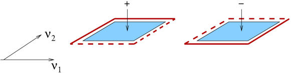
Figure 1: Plaquette update: A plaquette occupation number is changed by $+1$ (lhs. plot) or $-1$ (rhs.) and the links of the plaquette are changed simultaneously. The full line indicates an increase by +1 and a dashed line a decrease by $-1$. The directions $1\leq\nu_{1}<\nu_{2}\leq 4$ indicate the plane of the plaquette.

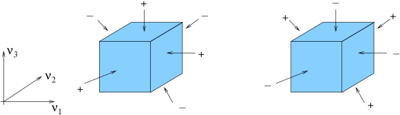
Figure 2: Cube update: Here we show the changes in the plaquette occupation numbers. The edges of the 3-cube are parallel to the directions $1\leq\nu_{1}<\nu_{2}<\nu_{3}\leq 4$.

Instead of the plaquette and cube updates we can use the worm algorithm. The SWA (see [6] for a detailed description) is constructed by breaking up the plaquette update into smaller building blocks called “segments” (examples are shown in Fig. 3) used to grow surfaces on which the flux and plaquette variables are changed. In the SWA the constraints are temporarily violated at a link $L_{V}$, the head of the worm, and the two sites at its endpoints. The admissible configurations are produced using 3 steps: The worms starts by changing the flux by $\pm 1$ at a randomly chosen link $L_{0}$ (step 1 in Fig. 4). $L_{0}$ becomes the head of the worm $L_{V}$. The defect at $L_{V}$ is then propagated through the lattice by attaching segments, which are chosen in such a way that the constraints are always obeyed (2 in Fig. 4). The defect is propagated through the lattice until the worm decides to end with the insertion of another unit of link flux at $L_{V}$ (3 in Fig. 4). A full sweep with the SWA consists of $V_{4}$ worms.

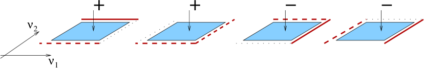
Figure 3: Examples of positive (lhs.) and negative segments (rhs.) in the $\nu_{1}$-$\nu_{2}$-plane ($\nu_{1}<\nu_{2}$). The plaquette occupation numbers are changed as indicated by the signs. The full (dashed) links are changed by $+1$ ($-1$). The empty link shows where the segment is attached to the worm and the dotted link is the new position of the link $L_{V}$ where the constraints are violated.

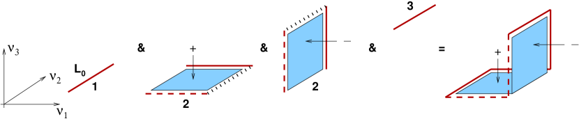
Figure 4: Illustration of the worm algorithm. See text for an explanation.

4 Numerical analysis

For the comparison of both algorithms we analyzed the bulk observables (and their fluctuations): $U_{P}$ which is the derivative wrt. $\beta$ and $|\phi|^{2}$ (derivative wrt. $\kappa$). First we checked the correctness of the SWA comparing the results for different lattices sizes and parameters. For example, the upper plot of Fig. 5 shows $U_{P}$ as a function of $\beta$ for $\kappa=4$, $\lambda=1.5$ on a lattice of size $4^{4}$. The lower plot shows $\langle|\phi|^{2}\rangle$ for $\kappa=8$ and $\lambda=1$ on a $10^{4}$ lattice. In both cases we used $10^{6}$ equilibration sweeps, $10^{6}$ measurements and $10$ sweeps for decorrelation between measurements. We observe very good agreement among the different algorithms.

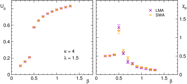
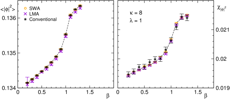
Figure 5: Observables as a function of $\beta$ for different parameters and volumes. We compare results from three algorithms: The conventional approach (asterisks), the SWA (circles) and the LMA (crosses).

In order to obtain a measure of computational effort, we compared the normalized autocorrelation time $\overline{\tau}$ as defined in [6] of the SWA and LMA for different volumes and parameters. We concluded that, the SWA outperforms the local update near a phase transition and if the acceptance rate of the link variable $l$ is not very low (eg. lhs. of Fig. 6). On the other hand, when the links become expensive the worm algorithm has difficulties to efficiently sample the system (as can be observed on the rhs. of Fig. 6, $\overline{\tau}$ for $U_{P}$ is larger for the SWA than for the LMA). But this can be overcome by offering a sweep of cube updates or a worm made of only plaquettes as described in [2].

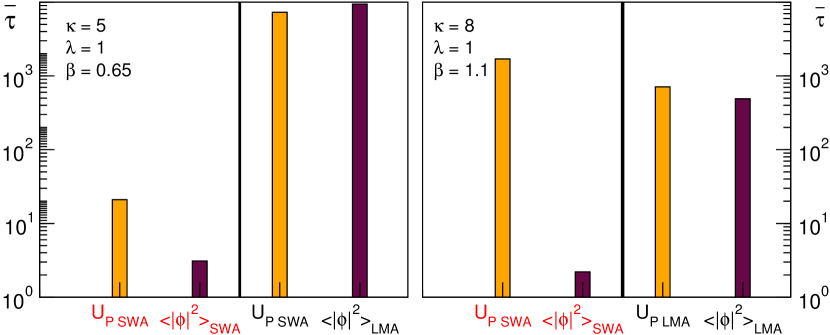
Figure 6: Normalized autocorrelation times $\overline{\tau}$ for 2 different set of parameters. Left: parameters close to a first order phase transition. Right: low acceptance rate of the variable $l$. Both simulations correspond to a $16^{4}$ lattice. Data taken from [6].

References

- [1] G. Aarts, PoS LATTICE 2012 (2012) 017 [arXiv:1302.3028 [hep-lat]]. P. de Forcrand, PoS LAT 2009 (2009) 010 [arXiv:1005.0539 [hep-lat]].
- [2] M.G. Endres, Phys. Rev. D 75 (2007) 065012 [hep-lat/0610029]; PoS LAT 2006, 133 (2006), [hep-lat/0609037].
- [3] C. Gattringer and A. Schmidt, Phys. Rev. D 86 (2012) 094506 [arXiv:1208.6472 [hep-lat]]. A. Schmidt, Y. Delgado and C. Gattringer, PoS LATTICE 2012 (2012) 098 [arXiv:1211.1573 [hep-lat]].
- [4] N. Prokof’ev and B. Svistunov, Phys. Rev. Lett. 87 (2001) 160601.
- [5] Y. Deng, T.M. Garoni and A.D. Sokal, Phys. Rev. Lett. 99 (2007) 110601 [cond-mat/0703787 [cond-mat.stat-mech]].
- [6] Y. D. Mercado, C. Gattringer and A. Schmidt, Comput. Phys. Commun. 184 (2013) 1535.
- [7] Y. D. Mercado, C. Gattringer and A. Schmidt, In preparation.