Single-particle and many-body analyses of a quasiperiodic integrable system after a quench

Abstract

In general, isolated integrable quantum systems have been found to relax to an apparent equilibrium state in which the expectation values of few-body observables are described by the generalized Gibbs ensemble. However, recent work has shown that relaxation to such a generalized statistical ensemble can be precluded by localization in a quasiperiodic lattice system. Here we undertake complementary single-particle and many-body analyses of noninteracting spinless fermions and hard-core bosons within the Aubry-André model to gain insight into this phenomenon. Our investigations span both the localized and delocalized regimes of the quasiperiodic system, as well as the critical point separating the two. Considering first the case of spinless fermions, we study the dynamics of the momentum distribution function and characterize the effects of real-space and momentum-space localization on the relevant single-particle wave functions and correlation functions. We show that although some observables do not relax in the delocalized and localized regimes, the observables that do relax in these regimes do so in a manner consistent with a recently proposed Gaussian equilibration scenario, whereas relaxation at the critical point has a more exotic character. We also construct various statistical ensembles from the many-body eigenstates of the fermionic and bosonic Hamiltonians and study the effect of localization on their properties.

I Introduction

In recent years, there has been a dramatic growth in interest in the physics of nonequilibrium quantum systems, driven in large part by advances in experimental atomic physics, in particular in the area of optical lattices Bloch et al. (2008); Cazalilla et al. (2011). The precision time-dependent control and observation of quantum effects afforded by these experiments, together with the high degree of isolation of the system from the environment, have invigorated the theoretical study of the time evolution of isolated many-body quantum systems. The predictions of previously abstract lines of theoretical inquiry into the mechanisms by which thermal behavior emerges from purely unitary time evolution, and the role of conservation laws and integrability in such dynamics, can now be directly compared with empirical evidence acquired in experimental laboratories.

Several theoretical studies into the quantum origins of thermalization in isolated nonintegrable systems have found that, away from the edges of the spectrum, few-body observables relax to the predictions of conventional statistical ensembles Deutsch (1991); Srednicki (1994); Rigol et al. (2008); Rigol (2009a, b); Biroli et al. (2010); Neuenhahn and Marquardt (2012); Steinigeweg et al. (2013), a phenomenon which has been connected Santos and Rigol (2010a, b) to the emergence of quantum chaos zel ; Zelevinsky et al. (1996); Flambaum et al. (1996); Flambaum and Izrailev (1997); BGI ; I (01). In addition, it is now well established that the highly constrained dynamics of integrable systems can in fact give rise to the relaxation of few-body observables, and that the equilibrium values of these quantities are in many cases described by the generalized Gibbs ensemble (GGE) Rigol et al. (2007, 2006); Cazalilla (2006); Calabrese and Cardy (2007); Kollar and Eckstein (2008); Iucci and Cazalilla (2009, 2010); Mossel and Caux (2010); Fioretto and Mussardo (2010); Cassidy et al. (2011); Calabrese et al. (2011); Cazalilla et al. (2012); Calabrese et al. (2012a, b); Gramsch and Rigol (2012); Ziraldo et al. (2012); Ziraldo and Santoro (2013).

The GGE is constructed by maximizing the many-body entropy Jaynes (1957a, b) while constraining the mean values of all integrals of motion to their expectation values in the initial state $|\Psi_{I}\rangle$ of the system. The density matrix in the GGE takes a Gaussian form similar to that of the grand-canonical ensemble, and can be written as Rigol et al. (2007)

$$\hat{\rho}_{\rm GGE}=\frac{1}{Z_{\rm GGE}}e^{-\sum_{s}\varLambda_{s}\hat{I}_{s}},$$ (1)

where $Z_{\rm GGE}=\textrm{Tr}[e^{-\sum_{s}\varLambda_{s}\hat{I}_{s}}]$ is the GGE partition function, the $\hat{I}_{s}$ are the conserved integrals of motion, and the $\varLambda_{s}$ are the corresponding Lagrange multipliers, which are determined by the constraints $\textrm{Tr}[\hat{\rho}_{\rm GGE}\,\hat{I}_{s}]=\langle\Psi_{I}|\hat{I}_{s}|\Psi_{I}\rangle$.

The significance of the fact that the GGE provides an accurate description of observables following relaxation can be seen by contrasting its predictions with those of the “diagonal ensemble” (DE) Rigol et al. (2008): for any initial state $|\Psi_{I}\rangle$, the time evolution of an observable $\hat{O}$ under a time-independent (integrable or nonintegrable) Hamiltonian $\hat{H}$ can be written as

$$O(\tau)=\sum_{\alpha}|C_{\alpha}|^{2}O_{\alpha\alpha}+\sum_{\alpha\neq\beta}{C^{*}_{\alpha}}C_{\beta}e^{i(E_{\alpha}-E_{\beta})\tau/\hbar}O_{\alpha\beta},$$ (2)

where $O(\tau)=\langle\Psi(\tau)|\hat{O}|\Psi(\tau)\rangle$, $|\Psi(\tau)\rangle=\sum_{\alpha}C_{\alpha}e^{-iE_{\alpha}\tau/\hbar}|\psi_{\alpha}\rangle$, $\hat{H}|\psi_{\alpha}\rangle=E_{\alpha}|\psi_{\alpha}\rangle$, $C_{\alpha}=\langle\psi_{\alpha}|\Psi_{I}\rangle$, and $O_{\alpha\beta}=\langle\psi_{\alpha}|\hat{O}|\psi_{\beta}\rangle$. The infinite-time average of the observable is therefore given by

$$\overline{O(\tau)} =\lim_{\tau^{\prime}\rightarrow\infty}\frac{1}{\tau^{\prime}}\int^{\tau^{\prime}}_{0}d\tau\,O(\tau)$$

$$=\sum_{\alpha}|C_{\alpha}|^{2}O_{\alpha\alpha}\equiv\langle\hat{O}\rangle_{\rm DE},$$ (3)

which defines the expectation value of $\hat{O}$ in the DE Rigol et al. (2008). The DE involves as many constraints as the dimension of the many-body Hilbert space (the overlaps of the initial state with the eigenstates of $\hat{H}$), which grows exponentially with system size. By contrast, for models that can be mapped to noninteracting Hamiltonians, the GGE involves a number of constraints that is only polynomially large in the size of the system Rigol et al. (2007). It may, therefore, appear surprising that the predictions of the GGE for expectation values of observables can agree with those of the DE.

From a many-body perspective, the success of the GGE can be understood as follows Cassidy et al. (2011): the eigenstates of a given integrable Hamiltonian with similar distributions of conserved quantities have similar expectation values of few-body observables (with the differences vanishing in the thermodynamic limit). Furthermore, the majority of the states that contribute to the DE have a distribution of conserved quantities similar (in a coarse-grained sense) to that of the initial state, and this is also the case for the states that contribute most strongly to the GGE. These facts imply that differences between the weights in the DE and the GGE are irrelevant and both ensembles will produce the same results for few-body observables in the thermodynamic limit Cassidy et al. (2011). This scenario can be viewed as a generalization of the eigenstate thermalization hypothesis Deutsch (1991); Srednicki (1994); Rigol et al. (2008), and has been explored in Ref. Caux and Essler for describing observables after relaxation by means of a single representative state.

Interestingly, it has been recently shown that in an integrable system, in the presence of localization, the GGE can fail to describe observables after relaxation Gramsch and Rigol (2012). This effect, which parallels the breakdown of eigenstate thermalization in nonintegrable disordered lattice systems in the presence of localization Khatami et al. (2012), has been related to the localized behavior of the underlying system of noninteracting particles to which some integrable models can be mapped Cazalilla et al. (2012); Ziraldo et al. (2012); Ziraldo and Santoro (2013). Here we gain further insights into this phenomenon by undertaking single-particle and many-body analyses of noninteracting spinless fermions and hard-core bosons. We study the dynamics of noninteracting fermions within the Aubry-André model previously studied in Ref. Gramsch and Rigol (2012) for hard-core bosons, and show that although the fermion momentum distribution equilibrates in the localized regime, it fails to equilibrate in the delocalized one. This should be contrasted with the density profiles, which exhibit the opposite behavior, equilibrating in the delocalized regime, but not in the localized regime Gramsch and Rigol (2012). We find that, whenever observables do equilibrate to their GGE values, they do so in a manner consistent with the Gaussian equilibration scenario of Ref. Campos Venuti and Zanardi (2013). Furthermore, we relate the failure of a given quantity to equilibrate in a certain regime to the behavior of the single-particle wave functions, as discussed in Refs. Cazalilla et al. (2012); Ziraldo et al. (2012); Ziraldo and Santoro (2013).

For hard-core bosons, we connect the results of Ref. Gramsch and Rigol (2012), in which the GGE was shown to fail to describe the momentum distribution function after relaxation in the localized regime, to the single-particle results for fermions. In addition, for both hard-core bosons and spinless fermions, we study the density profiles and momentum distribution functions in the many-body eigenstates of the appropriate Hamiltonians. We focus in particular on the behavior of these quantities in the many-body eigenstates that contribute to the DE, to the microcanonical ensemble (ME), and to the microcanonical version of the GGE, i.e., the generalized microcanonical ensemble (GME) Cassidy et al. (2011). We find indications that single-particle real-space localization in the localized phase and momentum-space localization in the delocalized phase lead to a distinctive behavior of the many-body eigenstate expectation values of the density and the momentum distribution of the fermions, respectively. No similar effect is detected in the many-body eigenstate expectation values of the momentum distribution of the hard-core bosons.

This paper is organized as follows. In Sec. II, we introduce the models, quench protocols, and observables studied in later sections. We also review the statistical ensembles utilized to describe observables after relaxation. The time evolution of spinless fermions following a quench is studied in Sec. III. Specifically, we examine the relaxation dynamics and time fluctuations of one-body observables, as well as properties of the single-particle eigenstates that help us understand the observed out-of-equilibrium behavior. Section IV is devoted to the study of one-particle observables in the many-body eigenstates of the bosonic and fermionic Hamiltonians. In Sec. V, we summarize our results and present our conclusions.

II Models and quenches

We consider two models on a one-dimensional lattice with open boundary conditions: noninteracting spinless fermions (SFs) and hard-core bosons (HCBs). The HCB model can be mapped onto the model of SFs, by mapping it first onto a spin-1/2 chain via the Holstein-Primakoff transformation Holstein and Primakoff (1940) and then onto SFs via the Jordan-Wigner transformation Jordan and Wigner (1928). In both cases, we study the effects of an additional periodic potential, with a period incommensurate with that of the underlying lattice of the tight-binding model, which results in the well known Aubry-André model Aubry and André (1980). The Hamiltonians for SFs and HCBs are given by

$${\hat{H}}_{f}=-t\sum_{j=1}^{L-1}\left({\hat{f}}_{j}^{\dagger}{\hat{f}}_{j+1}+\text{H.c.}\right)+\lambda\sum_{j=1}^{L}\cos(2\pi\varsigma j){\hat{n}}_{j}^{f},$$ (4)

and

$${\hat{H}}_{b}=-t\sum_{j=1}^{L-1}\left({\hat{b}}_{j}^{\dagger}{\hat{b}}_{j+1}+\text{H.c.}\right)+\lambda\sum_{j=1}^{L}\cos(2\pi\varsigma j){\hat{n}}_{j}^{b},$$ (5)

respectively, where $L$ is the length of the lattice, ${\hat{f}}_{j}$ and ${\hat{f}}_{j}^{\dagger}$ (${\hat{b}}_{j}$ and ${\hat{b}}_{j}^{\dagger}$) are fermionic (bosonic) annihilation and creation operators on site $j$, and ${\hat{n}_{j}}^{f}={\hat{f}}_{j}^{\dagger}{\hat{f}}_{j}$ (${\hat{n}}_{j}^{b}={\hat{b}}_{j}^{\dagger}{\hat{b}}_{j}$) are SF (HCB) site-occupation number operators. The prohibition of multiple occupancy of a single site for HCBs is enforced by the hard-core constraint $\hat{b}_{j}^{\dagger 2}=\hat{b}_{j}^{2}=0$. We denote the hopping parameter by $t$, and the strength of the incommensurate potential by $\lambda$. To ensure the incommensurability of the lattice potential, we use an irrational value for $\varsigma$. We select the inverse golden mean, $\varsigma=(\sqrt{5}-1)/2$, which is considered to be the most irrational number Sokoloff (1985). For each given system size, we take the total number of SFs (HCBs) $N_{f}$ ($N_{b}$) to be $N_{f}=N_{b}\equiv N$. In what follows we set $t$ to unity; i.e., we take $t$ as our unit of energy, and we also set $\hbar=1$ and the Boltzmann constant $k_{B}=1$.

The fermionic Hamiltonian (4) is quadratic and therefore trivially solvable: all many-body eigenstates can be constructed as Slater determinants of the single-particle energy eigenstates in the incommensurate periodic potentials. Although the bosonic Hamiltonian (5) is also superficially quadratic, the hard-core constraints on the bosonic creation and annihilation operators encode interactions between the bosons, precluding a direct diagonalization in terms of single-particle states. Nevertheless, it can be solved via the combined Holstein-Primakoff and Jordan-Wigner transformations, which implies that SF and HCB systems with Hamiltonians Eqs. (4) and (5), respectively, share the same (many-body) energy spectrum and consequently have identical thermodynamic properties. Moreover, the two models have identical site occupations ${\hat{n}_{j}}^{f}={\hat{n}}_{j}^{b}\equiv{\hat{n}_{j}}$.

The properties of HCBs in the Aubry-André model have previously been investigated, at both zero Rey et al. (2006); He et al. (2012) and finite temperature Nessi and Iucci (2011). The single-particle Aubry-André model exhibits a localization-delocalization transition at the critical potential strength $\lambda_{c}=2$ Aubry and André (1980): All single-particle states are extended when $\lambda<\lambda_{c}$ and exponentially localized when $\lambda>\lambda_{c}$. At the critical point, the energy spectrum exhibits the fractal structure of a Hofstadter butterfly Hofstadter (1976). As HCBs can be mapped onto noninteracting fermions, they of course inherit this phase transition when subjected to the incommensurate Aubry-André potential. In the localized regime, correlations in the ground state of the bosonic system decay exponentially with spatial separation, and the system is said to form a Bose glass Cazalilla et al. (2011).

Here we study the dynamics and behavior of observables following sudden quenches of the incommensurate lattice strength $\lambda$. We choose as our initial states $|\Psi_{I}\rangle$ the ground states of initial Hamiltonians ${\hat{H}}_{I}$ with parameters $\lambda_{I}$, and consider the ensuing dynamics generated by final Hamiltonians ${\hat{H}}_{F}$ with parameters $\lambda_{F}$, corresponding to an instantaneous change (quench) of the lattice strength from $\lambda_{I}$ to $\lambda_{F}$. We focus on one-body observables that are accessible in optical lattice experiments: the density profiles ${\hat{n}}_{j}$, and the momentum distribution functions

$$\hat{m}^{f}_{k}=\frac{1}{L}\sum_{j,j^{\prime}=1}^{L}e^{ik(j-j^{\prime})}{\hat{f}}_{j}^{\dagger}{\hat{f}}_{j^{\prime}}$$ (6)

and

$$\hat{m}^{b}_{k}=\frac{1}{L}\sum_{j,j^{\prime}=1}^{L}e^{ik(j-j^{\prime})}{\hat{b}}_{j}^{\dagger}{\hat{b}}_{j^{\prime}}.$$ (7)

We note that although the site occupations are equal for SFs and HCBs, the off-diagonal spatial correlations, and therefore the momentum distributions, of the two systems are distinct. To calculate $\langle\hat{m}^{b}_{k}\rangle$ in a pure state, we follow the approach of Refs. Rigol and Muramatsu (2004, 2005); He and Rigol (2011), while for calculations in the GGE we use the methodology of Ref. Rigol (2005).

Ensembles of interest

We characterize the behavior of our quasiperiodic system after relaxation following a quench by comparing it to three different statistical ensembles: DE, ME, and GME, each of which we briefly describe here.

Diagonal ensemble. The density matrix of the DE is defined by

$$\hat{\rho}_{\text{DE}}=\lim_{\tau^{\prime}\rightarrow\infty}\frac{1}{\tau^{\prime}}\int^{\tau^{\prime}}_{0}d\tau\,|\Psi(\tau)\rangle\langle\Psi(\tau)|=\sum_{\alpha}|C_{\alpha}|^{2}|\psi_{\alpha}\rangle\langle\psi_{\alpha}|,$$ (8)

i.e., it is diagonal in the (many-body) energy representation, and the energy eigenstates are weighted according to their overlaps with the initial state. The expectation value of an observable in this ensemble is given by Eq. (I). In various computational studies Rigol (2009a, b); Cassidy et al. (2011), observables after relaxation have been shown to approach the DE predictions [Eq. (I)] as the system size increases.

Microcanonical ensemble. The density matrix of the ME can be written as

$$\hat{\rho}_{\text{ME}}=\frac{1}{{\cal N}_{E,\delta_{\textrm{ME}}}}\sum_{\underset{|E-E_{\alpha}|<\delta_{\textrm{ME}}}{\alpha}}|\psi_{\alpha}\rangle\langle\psi_{\alpha}|;$$ (9)

i.e., all eigenstates in the energy window $[E-\delta_{\textrm{ME}},E+\delta_{\textrm{ME}}]$ (of which there are ${\cal N}_{E,\delta_{\textrm{ME}}}$) are given equal weight. We have checked that expectation values of observables within our microcanonical calculations are robust against the exact value of $\delta_{\textrm{ME}}$. To ensure this, we select $\delta_{\textrm{ME}}$ to be much smaller than the full spectrum width, but sufficiently large to contain many eigenstates (i.e., larger than the average level spacing at the given $E$). In general, $\delta_{\mathrm{ME}}=0.05$ for most results reported in this work.

Generalized Gibbs ensemble. The density matrix for this ensemble, which is of a similar Gaussian form to that of the grand-canonical ensemble, was already introduced in Eq. (1). We note that a recipe for constructing the appropriate conserved quantities, allowing for the extension of the GGE description to more general systems than those considered in this article, has recently been proposed Olshanii . However, we make here the “natural” choice for the conserved quantities, taking them to be the occupations of the single-particle eigenstates of the noninteracting SFs Rigol et al. (2007).

Generalized microcanonical ensemble. The GME is the microcanonical version of the GGE Cassidy et al. (2011). The only energy eigenstates that contribute to this ensemble are those that have distributions of the conserved quantities that are similar (in a coarse-grained sense) to that of the initial state. These eigenstates are all assigned the same weight, as in the usual ME. The density matrix of the GME therefore has the form

$$\hat{\rho}_{\textrm{GME}}=\frac{1}{{\cal N}_{\{I_{s}\},\delta_{\textrm{GME}}}}\sum_{\underset{\delta_{\alpha}<\delta_{\textrm{GME}}}{\alpha}}|\psi_{\alpha}\rangle\langle\psi_{\alpha}|,$$ (10)

where $\delta_{\alpha}$ measures the distance of the eigenstate $|\psi_{\alpha}\rangle$ from the target distribution of conserved quantities determined by the initial state, and ${\cal N}_{\{I_{s}\},\delta_{\textrm{GME}}}$ is the number of energy eigenstates within the GME window $\delta_{\alpha}<\delta_{\textrm{GME}}$.

In order to construct the GME, one needs to compare the distribution of conserved quantities in each of the eigenstates of ${\hat{H}}_{F}$ with that of the initial state. Since the conserved quantities are fermion occupation numbers of single-particle energy eigenstates, their expectation values $I_{s,\alpha}=\langle\psi_{\alpha}|\hat{I}_{s}|\psi_{\alpha}\rangle$ in the many-body eigenstates are either 0 or 1. By contrast, the occupations of the conserved quantities in the initial state (which are equal to those in the DE) can assume any real value between these two values; i.e., $0\leq\langle\hat{I}_{s}\rangle_{\textrm{DE}}=\sum_{\alpha}|C_{\alpha}|^{2}I_{s,\alpha}\leq 1$. To compare those distributions, in a coarse-grained way, we proceed as follows Cassidy et al. (2011).

(i) We sort the conserved quantities so that $\langle\hat{I}_{s}\rangle_{\textrm{DE}}$ decreases monotonically as $s$ increases. In this way we obtain a comparatively smoothly varying discrete distribution suitable for coarse graining.

(ii) After sorting, we generate a discrete target distribution of conserved quantities from $\langle\hat{I}_{s}\rangle_{\textrm{DE}}$. This is achieved by interpolating $\langle\hat{I}_{s}\rangle_{\textrm{DE}}$ to find a continuous function $I(s)$ (where $s$ can now be any real number in the interval [$0.5,L+0.5$]), and then computing all values $s_{l}^{*}$ satisfying $\int_{0.5}^{s_{1}^{*}}I(s)\,ds=0.5$ and $\int_{s_{l-1}^{*}}^{s_{l}^{*}}I(s)\,ds=1$ for $l>1$. The set $\{s_{l}^{*}\}$, together with the set of corresponding weights $\{I(s_{l}^{*})\}$, defines the target distribution.

(iii) We introduce a measure $\delta_{\alpha}$ to quantify how close the distribution of each many-body eigenstate $|\psi_{\alpha}\rangle$ is to the target distribution. Those states with $\delta_{\alpha}<\delta_{\textrm{GME}}$ are included in the GME. The choice of $\delta_{\alpha}$ is not unique. Following Ref. Cassidy et al. (2011), we choose

$$\delta_{\alpha}=\sqrt{\frac{1}{N}\sum_{l=1}^{N}I(s_{l}^{*})(s_{l,\alpha}-s_{l}^{*})^{2}},$$ (11)

where $s_{l,\alpha}$, with $l=1,\ldots,N$, enumerate the sorted single-particle states [see (i)] occupied in eigenstate $|\psi_{\alpha}\rangle$. We choose the value of $\delta_{\textrm{GME}}$ to be that which yields the minimum value of the normalized absolute difference

$$D=\frac{\sum_{s=1}^{L}|\langle\hat{I}_{s}\rangle_{\textrm{GME}}-\langle\hat{I}_{s}\rangle_{\textrm{DE}}|}{\sum_{s=1}^{L}\langle\hat{I}_{s}\rangle_{\textrm{DE}}},$$ (12)

between the expectation values of the conserved quantities in the GME and DE. As in our microcanonical calculations, we have checked that our results are robust against small changes in the value of $\delta_{\textrm{GME}}$.

III Single-particle analysis

In Ref. Gramsch and Rigol (2012) it was shown that, following a quench of HCBs to the localized regime of the Aubry-André model, one-body observables that depend on nonlocal correlations, such as $m^{b}_{k}$, do relax to time-independent values (with fluctuations vanishing in the thermodynamic limit), but these values are not consistent with the predictions of the GGE. This should be contrasted with the on-site density, whose time average agrees with the GGE results in all regimes. It was also found that the dynamics of $n_{j}$ and $m^{b}_{k}$ are qualitatively different in the delocalized and localized regimes: the momentum distribution $m^{b}_{k}$ approaches a time-independent value with increasing system size regardless of whether the system is in the delocalized or localized regime, while $n_{j}$ only exhibits such relaxation in the delocalized regime. All results for the density also apply to SFs, to which HCBs can be mapped.

Here, we begin by studying the relaxation dynamics of the momentum distribution $m_{k}^{f}$ of SFs, which is in general completely unrelated to the momentum distribution of the corresponding system of HCBs. In fact, the GGE describes, by construction, the infinite-time averages of all one-body fermionic observables regardless of whether the single-particle states are localized or delocalized and independently of the system size. This can be straightforwardly proven by projecting $\hat{\rho}(\tau)=|\Psi(\tau)\rangle\langle\Psi(\tau)|$ onto the single-particle sector. Considering that all eigenstates of the many-body Hamiltonian are (antisymmetrized) direct products of the single-particle states $|s\rangle$ in which $\hat{H}_{f}$ is diagonal ($\hat{H}_{f}|s\rangle=e_{s}|s\rangle$), the time evolution of the one-particle density matrix can be cast in the form

$$\hat{\rho}_{\text{sp}}(\tau)=\sum_{s,s^{\prime}}c_{ss^{\prime}}e^{-i(e_{s}-e_{s^{\prime}})\tau}|s\rangle\langle s^{\prime}|.$$ (13)

In the absence of degeneracies in the single-particle spectrum (which is the case in the Aubry-André model considered here), the infinite-time average of $\hat{\rho}_{\text{sp}}(\tau)$ can be written as

$$\overline{\hat{\rho}_{\text{sp}}(\tau)}=\lim_{\tau^{\prime}\rightarrow\infty}\frac{1}{\tau^{\prime}}\int^{\tau^{\prime}}_{0}d\tau\,\hat{\rho}_{\text{sp}}(\tau)=\sum_{s}c_{ss}|s\rangle\langle s|,$$ (14)

which is, by construction, the single-particle density matrix predicted by the GGE, as $c_{ss}=\sum_{\alpha}|C_{\alpha}|^{2}I_{s,\alpha}\equiv\textrm{Tr}[\hat{\rho}_{\rm GGE}\,\hat{I}_{s}]$. We emphasize, however, that this does not necessarily imply that all such observables exhibit relaxation to their GGE values. In particular, the results of Ref. Gramsch and Rigol (2012) indicate that the on-site densities in the localized phase exhibit finite fluctuations about their GGE expectation values even in the thermodynamic limit.

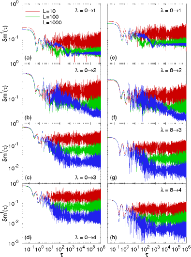
Figure 1: (Color online) Relaxation dynamics of $m^{f}_{k}$ in quenches $\lambda=\lambda_{I}\rightarrow\lambda_{F}$ (as indicated in the panels) for systems with 10, 100, and 1000 lattice sites (curves from top to bottom in each panel), and $N=L/2$.

In order to quantify how closely $m_{k}^{f}(\tau)=\langle\Psi(\tau)|\hat{m}_{k}^{f}|\Psi(\tau)\rangle$ approaches the corresponding GGE prediction, we compute the normalized difference

$$\delta m^{f}(\tau)=\frac{\sum_{k}|m_{k}^{f}(\tau)-\langle\hat{m}_{k}^{f}\rangle_{\text{GGE}}|}{\sum_{k}\langle\hat{m}_{k}^{f}\rangle_{\text{GGE}}},$$ (15)

between the instantaneous momentum distribution at time $\tau$ and the GGE prediction for this quantity. Relaxation of $m_{k}^{f}$ to the GGE prediction is observed if $\delta m^{f}(\tau)$ vanishes at long times, in the thermodynamic limit. In practical numerical calculations, however, $\delta m^{f}(\tau)$ will always be finite, because of finite-size effects. The signature of relaxation to the GGE in our calculations is therefore that $\delta m^{f}(\tau)$ fluctuates about a finite average value at long times, and that this average value scales towards zero with increasing system size.

In Fig. 1, we show results for $\delta m^{f}(\tau)$ in quenches with $\lambda_{I}=0$; i.e., a delocalized initial state (left panels), and $\lambda_{I}=8$; i.e., a localized initial state (right panels). After the quench, $\lambda_{F}=1$ [delocalized regime, Figs. 1(a) and 1(e)], $\lambda_{F}=2$ [critical point, Figs. 1(b) and 1(f)], and $\lambda_{F}=3$ and 4 [localized regime, Figs. 1(c), 1(g), and 1(d), 1(h), respectively]. The results presented correspond to three different system sizes ($L=10,\,100,$ and 1000, curves from top to bottom in each panel, and $N=L/2$), and to the same quenches and system sizes studied for HCB systems in Ref. Gramsch and Rigol (2012).

The results obtained for a given final value of the incommensurate potential strength are qualitatively similar, independently of whether the initial state is delocalized or localized. In quenches to the localized regime [Figs. 1(c), 1(d), 1(g), and 1(h)], we observe that $\delta m^{f}(\tau)$ decays to a finite value, about which it undergoes fluctuations, and that this value decreases with increasing system size. In quenches to the delocalized regime [Figs. 1(a) and 1(e)], $\delta m^{f}(\tau)$ similarly undergoes decay to a finite value about which it fluctuates. However, in the delocalized case, the value to which $\delta m^{f}(\tau)$ decays does not appear to exhibit such a pronounced reduction as the system size is increased, suggesting that it may not tend towards zero as $L\to\infty$. Following quenches to the critical point [Figs. 1(b) and 1(f)], $\delta m^{f}(\tau)$ exhibits behavior similar to that observed in the localized regime, decaying to exhibit fluctuations about a constant value that decreases with increasing system size. However, in this critical regime the decay of $\delta m^{f}(\tau)$ is much slower and, e.g., fluctuation about a constant value in the case $L=1000$ is only obtained for $\tau\gtrsim 10^{5}$.

Figure 2: (Color online) Finite-size scaling of $\delta m^{f}(\infty)$ (see text) for the quenches studied in Fig. 1. Thin continuous lines depict power-law fits in which $\delta m^{f}(\infty)\propto L^{-0.25\pm 0.01}$ for quenches with $\lambda_{F}=\lambda_{c}$ and $\delta m^{f}(\infty)\propto L^{-0.500\pm 0.005}$ in quenches with $\lambda_{F}>\lambda_{c}$. The power laws were fitted to results with $L$ in the interval [200, 1000].

To gain a quantitative understanding of the dependence of the long-time behavior of Eq. (15) on the system size, we consider the average of $\delta m^{f}(\tau)$ over the time interval $\tau\in[10^{5},10^{6}]$, and denote this quantity by $\delta m^{f}(\infty)$. We regard $\delta m^{f}(\infty)$ as representative of the constant value about which $\delta m^{f}(\tau)$ fluctuates after any transient dynamics have subsided, and away from any revival. In Fig. 2, we plot $\delta m^{f}(\infty)$ against $L$ for all the quenches shown in Fig. 1. The scalings make apparent that $\delta m^{f}(\infty)$ converges to a finite value as the system size is increased in quenches to the delocalized phase; i.e., although the infinite time average of each $m^{f}_{k}$ trivially agrees with its expectation value in the GGE, its instantaneous value does not relax to the GGE in the thermodynamic limit. By contrast, in quenches to the localized regime $\delta m^{f}(\infty)$ decreases with increasing system size as a power law, which we find to be close to $L^{-0.50}$. In the quenches to the critical regime, $\delta m^{f}(\infty)$ is much slower to reach a clear power-law scaling, but for large system sizes its behavior is consistent with $\delta m^{f}(\infty)\propto L^{-0.25}$.

The behavior of $\delta m^{f}(\infty)$ in the delocalized and localized regimes is exactly opposite to that observed for the long-time average density difference Not in Refs. Gramsch and Rigol (2012). There it was found that the normalized difference of the density $\delta n(\infty)\propto L^{-0.5}$ in quenches to the delocalized phase, whereas it converges to a finite value in quenches to the localized phase. Intuitively, the extended states in the delocalized regime of the quasiperiodic lattice (and a fortiori those in a monochromatic lattice) can be thought of as states that are localized in momentum space. In fact, the correspondence between position (momentum) space results in the delocalized phase and momentum (position) space quantities in the localized phase can, in the case of free fermions, be seen to be an exact consequence of the well-known self-duality of the Aubry-André model Sokoloff (1985). We note also that the behavior of $\delta m^{f}(\infty)$ at the critical point is similar to that found for $\delta n(\infty)$ in Ref. Gramsch and Rigol (2012).

Aside from the peculiar behavior observed at the critical point, which is understandable given the very special character of the single-particle problem in this regime, it is remarkable that whenever relaxation of $n_{j}$ or $m^{f}_{k}$ takes place (in the delocalized or localized regime) the time fluctuations are proportional to $L^{-0.5}$. This is consistent with the Gaussian equilibration scenario of Ref. Campos Venuti and Zanardi (2013), in which the square root of the normalized time variance of one-body observables in noninteracting fermion systems was argued to scale as $1/\sqrt{L}$ not .

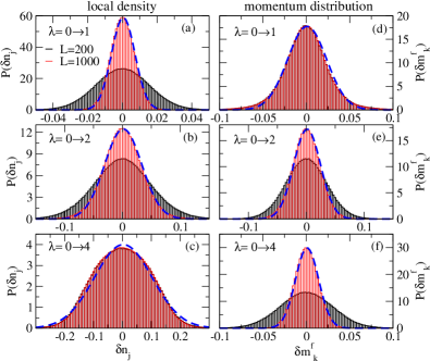
Figure 3: (Color online) Histograms of the time fluctuations of $n_{j}$ (left panels) and $m^{f}_{k}$ (right panels) in quenches with $\lambda_{I}=0$ and $\lambda_{F}=1$ (a),(d), $\lambda_{F}=2$ (b),(e), and $\lambda_{F}=4$ (c),(f). In all panels, we report results for systems with $L=200$ and $L=1000$, and Gaussian fits to the data for $L=1000$ (dashed lines). From the fits, the means were found to be zero ($\pm 0.003$) in all cases and the variances were found to be $\sigma=(6.770\pm 0.004)\times 10^{-3}$ (a), $(3.206\pm 0.009)\times 10^{-2}$ (b), $(1.008\pm 0.007)\times 10^{-1}$ (c), $(2.25\pm 0.02)\times 10^{-2}$ (d), $(2.322\pm 0.005)\times 10^{-1}$ (e), and $(1.336\pm 0.001)\times 10^{-2}$ (f).

In Figs. 3 and 4, we present histograms of the distributions of differences $\delta n_{j}(\tau)=n_{j}(\tau)-\langle\hat{n}_{j}\rangle_{\mathrm{GGE}}$ between the instantaneous values of the site occupations and their mean values in the GGE (left panels), and the analogous quantities $\delta m^{f}_{k}(\tau)=m^{f}_{k}(\tau)-\langle\hat{m}^{f}_{k}\rangle_{\mathrm{GGE}}$ calculated for momentum-mode occupations (right panels). These histograms represent the full distribution of fluctuations of the occupations of all lattice sites $j$, and all momentum modes $k$, in quenches with $\lambda_{I}=0$ (Fig. 3) and $\lambda_{I}=8$ (Fig. 4). Once again, the results for a given value of $\lambda_{F}$ can be seen to be qualitatively similar independently of the initial state. The histograms of the time fluctuations of $n_{j}$ in quenches to the delocalized regime and of $m^{f}_{k}$ in quenches to the localized regime have a Gaussian shape with a width that decreases with increasing system size. By contrast, the histograms of the time fluctuations of $n_{j}$ in quenches to the localized regime and of $m^{f}_{k}$ in quenches to the delocalized regime are in general non-Gaussian (as can be seen by comparing them to the indicated best Gaussian fits to the distributions) and the widths of the distributions are not seen to decrease with increasing system size. We note that the distributions of time fluctuations of individual lattice-site (momentum-mode) occupations in the localized (delocalized) phase, which we have not shown, are quite strongly non-Gaussian, exhibiting, e.g., bimodal structures. The behavior of the time fluctuations at the critical point is intermediate between what is seen in the localized and delocalized phases: the fluctuations of $n_{j}$ and $m^{f}_{k}$ are close to Gaussian, with a width that decreases less dramatically with increasing system size, consistent with the $L^{-0.25}$ behavior found for $\delta m^{f}(\infty)$ (Fig. 2). This exotic behavior at the critical point warrants a more specific investigation that is beyond the scope of this article.

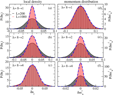
Figure 4: (Color online) Histograms of the time fluctuations of $n_{j}$ (left panels) and $m^{f}_{k}$ (right panels) in quenches with $\lambda_{I}=8$ and $\lambda_{F}=1$ (a),(d), $\lambda_{F}=2$ (b),(e), and $\lambda_{F}=4$ (c),(f). In all panels, we report results for systems with $L=200$ and $L=1000$, and Gaussian fits to the data for $L=1000$ (dashed lines). From the fits, the means were found to be zero ($\pm 0.003$) in all cases and the variances were found to be $\sigma=(1.2373\pm 0.0004)\times 10^{-2}$ (a), $(2.570\pm 0.008)\times 10^{-2}$ (b), $(2.27\pm 0.01)\times 10^{-2}$ (c), $(4.318\pm 0.005)\times 10^{-2}$ (d), $(1.860\pm 0.004)\times 10^{-2}$ (e), and $(3.360\pm 0.003)\times 10^{-3}$ (f).

An understanding of why Gaussian equilibration fails to occur for both fermionic observables at the critical point, for $m^{f}_{k}$ in the delocalized phase, and for $n_{j}$ in the localized one, can be gained through an analysis of the properties of the single-particle eigenstates of ${\hat{H}}_{f}$ ($|s\rangle=\hat{\gamma}^{\dagger}_{s}|0\rangle$) in both real and momentum space Cazalilla et al. (2012); Ziraldo et al. (2012); Ziraldo and Santoro (2013). Since the variances

$$\sigma^{2}_{n_{j}} = \lim_{\tau^{\prime}\rightarrow\infty}\frac{1}{\tau^{\prime}}\int^{\tau^{\prime}}_{0}d\tau\,[n_{j}(\tau)-\langle\hat{n}_{j}\rangle_{\textrm{GGE}}]^{2},$$

$$\sigma^{2}_{m_{k}} = \lim_{\tau^{\prime}\rightarrow\infty}\frac{1}{\tau^{\prime}}\int^{\tau^{\prime}}_{0}d\tau\,[m^{f}_{k}(\tau)-\langle\hat{m}^{f}_{k}\rangle_{\text{GGE}}]^{2},$$ (16)

can be written as

$$\sigma^{2}_{n_{j}} = \sum_{s\neq s^{\prime}}|u_{js}|^{2}|u_{js^{\prime}}|^{2}|\rho^{I}_{ss^{\prime}}|^{2},$$

$$\sigma^{2}_{m_{k}} = \sum_{s\neq s^{\prime}}|v_{ks}|^{2}|v_{ks^{\prime}}|^{2}|\rho^{I}_{ss^{\prime}}|^{2},$$ (17)

where $\rho^{I}_{ss^{\prime}}=\langle\Psi_{I}|\hat{\gamma}^{\dagger}_{s}\hat{\gamma}^{\phantom{\dagger}}_{s^{\prime}}|\Psi_{I}\rangle$, and $\hat{\gamma}^{\dagger}_{s}=\sum_{j}u_{js}\hat{f}^{\dagger}_{j}=\sum_{k}v_{ks}\hat{c}^{\dagger}_{k}$ ($\hat{c}^{\dagger}_{k}$ creates a SF at momentum $k$), it follows that Ziraldo et al. (2012): (i) if $|s\rangle$ is delocalized in real (momentum) space then $|u_{js}|^{2}\sim 1/L$ ($|v_{ks}|^{2}\sim 1/L$) and $\sigma^{2}_{n_{j}}$ ($\sigma^{2}_{m_{k}}$) must decrease as $1/L$ or faster (because $\sum_{s,s^{\prime}}|\rho^{I}_{ss^{\prime}}|^{2}=N_{f}$) with increasing system size, and (ii) if $|s\rangle$ is localized in real (momentum) space, then the corresponding variance $\sigma^{2}_{n_{j}}$ ($\sigma^{2}_{m_{k}}$) will be dominated by rare large values of $|\rho^{I}_{ss^{\prime}}|^{2}$ and will remain finite in the thermodynamic limit.

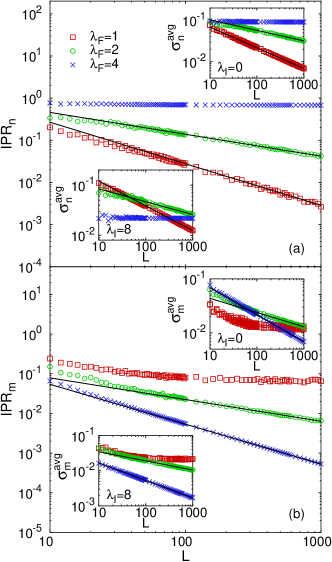
Figure 5: (Color online) Inverse participation ratios in real (a) and momentum space (b) in the delocalized and localized phases as well as at the critical point. Thin continuous lines are power-law fits in which (a) $\text{IPR}_{n}\propto L^{-0.99\pm 0.02}$ for $\lambda_{F}=1$ and $\text{IPR}_{n}\propto L^{-0.52\pm 0.01}$ for $\lambda_{F}=2$, and (b) $\text{IPR}_{m}\propto L^{-0.55\pm 0.01}$ for $\lambda_{F}=2$ and $\text{IPR}_{n}\propto L^{-1.005\pm 0.001}$ for $\lambda_{F}=4$. The insets in (a) depict $\sigma_{n}^{\text{avg}}$ for quenches with $\lambda_{I}=0$ (top inset) and $\lambda_{I}=8$ (bottom inset), while the insets in (b) depict $\sigma_{m}^{\text{avg}}$ for quenches with $\lambda_{I}=0$ (top inset) and $\lambda_{I}=8$ (bottom inset). Thin continuous lines are power-law fits in which, in both insets in (a), $\sigma_{n}^{\text{avg}}\propto L^{-0.50\pm 0.01}$ for $\lambda_{F}=1$ and $\sigma_{n}^{\text{avg}}\propto L^{-0.25\pm 0.01}$ for $\lambda_{F}=2$, and, in both insets in (b), $\sigma_{m}^{\text{avg}}\propto L^{-0.25\pm 0.02}$ for $\lambda_{F}=2$ and $\sigma_{m}^{\text{avg}}\propto L^{-0.500\pm 0.005}$ for $\lambda_{F}=4$. The power laws were fitted to results with $L$ in the interval [160, 1000].

In the insets to Fig. 5, we plot the average of the square root of the variance over all lattice sites $\sigma_{n}^{\text{avg}}=1/L\sum_{j}\sigma_{n_{j}}$ [insets in Fig. 5(a)] and over all momentum states $\sigma_{m}^{\text{avg}}=1/L\sum_{k}\sigma_{m_{k}}$ [insets in Fig. 5(b)] against the system size $L$, for systems with between 10 and 1000 lattice sites and subject to the same quenches studied previously ($\lambda_{I}=0$ in the top insets and $\lambda_{I}=8$ in the bottom ones). The results for $\sigma_{n}^{\text{avg}}$ and $\sigma_{m}^{\text{avg}}$ can be seen to be qualitatively similar to those in Ref. Gramsch and Rigol (2012) for $\delta n(\infty)$ and in Fig. 2 for $\delta m^{f}(\infty)$. In order to relate the behavior of the variances to the properties of the single-particle eigenstates $|s\rangle$ in real and momentum space, we compute the average inverse participation ratios (IPRs)

$$\text{IPR}_{n} = \frac{1}{L}\sum_{s}\sum_{j}|u_{js}|^{4},$$

$$\text{IPR}_{m} = \frac{1}{L}\sum_{s}\sum_{k}|v_{ks}|^{4}.$$ (18)

The results for the IPRs are reported in the main panels in Fig. 5. They show that, as expected, the eigenstates of the Hamiltonian are delocalized in real space ($\text{IPR}_{n}\sim 1/L$) and localized in momentum space ($\text{IPR}_{m}\sim L^{0}$) for $\lambda_{F}<2$, and localized in real space ($\text{IPR}_{n}\sim L^{0}$) and delocalized in momentum space ($\text{IPR}_{m}\sim 1/L$) for $\lambda_{F}>2$, which explains the behavior of the time fluctuations of the density and fermionic momentum distributions in the delocalized and localized regimes. For $\lambda_{F}=2$, we find that $\text{IPR}_{n}\sim\text{IPR}_{m}\sim 1/\sqrt{L}$, illustrating the exotic structure of the eigenstates of the critical Hamiltonian in both real and momentum space. From this scaling we can infer that $|u_{js}|^{2}\sim|v_{ks}|^{2}\sim 1/L^{0.75}$ when $\lambda_{F}=2$, implying that $\sigma_{n_{j}}^{2}$ and $\sigma_{m_{k}}^{2}$ decay like $1/\sqrt{L}$ or faster at the critical point, which is indeed consistent with the results of Fig. 2. We note also that in general, the average square-root variances and IPRs in the critical regime reach their exotic scaling limits at quite small values of $L$, compared to the behavior of $\delta m^{f}(\infty)$ at the critical point (Fig. 2). The unambiguous scaling at criticality seen in Fig. 5 thus lends strong support to our identification of $\delta m^{f}(\infty)$ as scaling like ${\sim}L^{-0.25}$ in this regime.

For fermionic observables, we should stress the fact that, in the localized regime, localization in real space precludes relaxation of the density profiles in the same way that, in the delocalized regime, localization in momentum space precludes relaxation of the momentum distribution. This symmetry between localization in real and momentum space is broken in the case of HCBs, because the mapping to the underlying model of SFs only preserves correlations that are diagonal in real space (i.e., properties related to the density). Thus for HCBs, although relaxation of the density is precluded in the localized regime, relaxation of the momentum distribution can occur in the delocalized regime, as was found in Ref. Gramsch and Rigol (2012).

As discussed in Refs. Cazalilla et al. (2012); Ziraldo et al. (2012); Ziraldo and Santoro (2013), if the variances of one-particle correlations (here we have focused only on the density and momentum distributions) do not vanish with increasing system size—which is only possible if off-diagonal elements of $|\rho^{I}_{ss^{\prime}}|^{2}$ contribute to the fluctuations in the thermodynamic limit—then Wick’s theorem can break down for time averages of higher-order correlations. We recall that nonlocal one-particle correlations of HCBs [e.g., Eq. (7)] correspond, via the Jordan-Wigner transformation, to higher-order correlations of SFs Ziraldo and Santoro (2013). Thus the breakdown of the GGE for describing $m^{b}_{k}$ after relaxation in the localized phase of HCBs Gramsch and Rigol (2012) can be understood as a direct consequence of the fact that time fluctuations of local one-particle correlations of the underlying free-fermion model remain finite as one increases the system size in the localized phase.

IV Many-Body Analysis

In this section, we study the density profiles and momentum distribution functions in the many-body eigenstates of the SF and HCB Hamiltonians. Our goal is to understand how localization, in real and momentum space, affects the many-body eigenstate expectation values of these observables. Since this study requires the construction of the full set of energy eigenstates of the many-body system, which grows exponentially with increasing system size, our analysis will be restricted to lattice lengths that are much smaller than those studied in the single-particle analysis of the previous section. The smallest systems considered in this section have 20 sites and the largest ones have $L=50$, and in each case $N=L/5$, in contrast to the filling $N=L/2$ (which yields the maximal Hilbert space dimension for a given system size) considered in the previous section. The largest systems we consider here have a Hilbert space of dimension $O(10^{10})$. In order to compare systems that have equivalent excitation energies per particle after the quench, we will focus on three quenches that, while having the same final Hamiltonians as in the previous section, have for their initial states the respective ground states of Hamiltonians with $\lambda_{I}=-1.5$ for $\lambda_{F}=1.0$, $\lambda_{I}=-0.5$ for $\lambda_{F}=2.0$, and $\lambda_{I}=1.0$ for $\lambda_{F}=4.0$. These three quenches lead to time-evolving states whose energies are similar to those of systems in thermal equilibrium with $T\sim 1.7$.

In Fig. 6, we show the distribution of conserved quantities in the quenches described above for systems with $L=50$. We compare results for those distributions in the initial state (same as the DE and the GGE), in the GME (constructed as described in Sec. II), and in the ME. The contrast between the distribution of conserved quantities in the initial state and in the ME is apparent, whereas the distribution in the GME closely agrees with that in the initial state. Figures 6(d)–6(i) depict how the normalized absolute differences between the distribution of conserved quantities in the GME and ME and that in the initial state [Eq. (12) and the analogous expression obtained by replacing $\langle\hat{I}_{s}\rangle_{\mathrm{GME}}$ with $\langle\hat{I}_{s}\rangle_{\mathrm{ME}}$, respectively] scale with increasing system size. For the systems analyzed here, these differences are always smaller for the GME than for the ME. More importantly, for all quenches, they are seen to decrease with increasing system size for the GME [Figs. 6(d), 6(f), and 6(h)]. The differences between the ME and the DE exhibit clear saturation behavior in the delocalized and critical regimes [Figs. 6(e) and 6(g)]. In the localized regime [Figs. 6(i)], the difference between the ME and DE is both smaller than, and does not exhibit saturation quite as obviously as, that in the other two regimes. We note, however, that it was found previously in Ref. Cassidy et al. (2011) that the discrepancy between distributions of conserved quantities in the ME and DE can be strongly dependent on the initial state (and in particular on its energy).

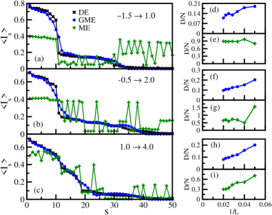
Figure 6: (Color online) [(a),(b),(c)] Conserved quantities $\langle\hat{I}_{s}\rangle$ in the DE, GME, and ME for $L=50$, $N=10$, sorted in order of decreasing occupation in the DE. [(d)–(i)] Scaling of the absolute differences $D$ between distributions of conserved quantities with increasing system size. [(d),(f),(h)] Absolute differences $D$ between the conserved quantities in the GME and the DE [see Eq. (12)]. [(e),(g),(i)] $D$ between the conserved quantities in the ME and the DE [same as Eq. (12) but with “GME”$\rightarrow$“ME”]. The quenches are indicated as $\lambda_{I}\rightarrow\lambda_{F}$. For quenches $\lambda_{I}=-1.5\rightarrow\lambda_{F}=1.0$ and $\lambda_{I}=-0.5\rightarrow\lambda_{F}=2.0$ we found that $\delta_{\textrm{GME}}=0.85$ yields the minimum value of $D$, and for quenches $\lambda_{I}=1.0\rightarrow\lambda_{F}=4.0$ we found $\delta_{\textrm{GME}}=0.95$. For the ME, $\delta_{\textrm{ME}}=0.05$ in all quenches.

Although disagreement between the distributions of conserved quantities in the DE and ME indicates the failure of the ME to describe the state of the system after relaxation, the degree of agreement between the corresponding distributions in the DE and GME yields only incomplete information on the accuracy of the GGE as a characterization of the system at long times. In particular, the distributions here apply equally to SFs and HCBs, whereas the results of Ref. Gramsch and Rigol (2012) and Sec. III indicate that the presence or absence of relaxation, and the agreement between time averages and the GGE predictions, can differ between SFs and HCBs with equal quench parameters. To further characterize the relationship between (generalized) thermalization and the structure of the many-body eigenstates of the system, we now turn our attention to the behavior of the density and momentum distributions in the eigenstates of the SF and HCB systems.

In order to quantify the differences between the predictions of the GME and ME for each observable and those of the DE, we compute the normalized difference,

$$\Delta O^{\textrm{stat-DE}}=\frac{\sum_{\ell}|O_{\textrm{stat},\ell}-O_{\textrm{DE},\ell}|}{\sum_{\ell}O_{\textrm{DE},\ell}},$$ (19)

where $O$ is either the site occupation $n$ (for which $\ell=j$) or the momentum occupation $m^{f}$ or $m^{b}$ (for which $\ell=k$), $O_{\textrm{stat},\ell}=\sum_{\alpha}w^{\textrm{stat}}_{\alpha}\langle\psi_{\alpha}|\hat{O}_{\ell}|\psi_{\alpha}\rangle\equiv\langle\hat{O}_{\ell}\rangle_{\textrm{stat}}$, with $w^{\textrm{stat}}_{\alpha}$ the weight of each many-body eigenstate in the relevant ensemble, and “stat” stands for one of the three ensembles: the DE, the GME, or the ME. Hence, the agreement between a statistical ensemble and the DE in the thermodynamic limit becomes apparent if $\Delta O^{\textrm{stat-DE}}$ vanishes with increasing system size.

We quantify the behavior of the eigenstate expectation values of the observables by calculating the average variance within each ensemble, which we define by

$$\sigma_{O}^{\textrm{stat}}=\frac{\sum_{\ell}\sqrt{(O^{2})_{\textrm{stat},\ell}-(O_{\textrm{stat},\ell})^{2}}}{L},$$ (20)

where $(O^{2})_{\textrm{stat},\ell}=\sum_{\alpha}w^{\textrm{stat}}_{\alpha}\langle\psi_{\alpha}|\hat{O}_{\ell}|\psi_{\alpha}\rangle^{2}\neq\langle\hat{O}^{2}_{\ell}\rangle_{\textrm{stat}}$ (cf. Refs. Rigol (2009a, b)). A finite value of ($\sigma_{O}^{\textrm{GME}}$) $\sigma_{O}^{\textrm{ME}}$ in the thermodynamic limit implies that (generalized) eigenstate thermalization does not occur. However, the vanishing of ($\sigma_{O}^{\textrm{GME}}$) $\sigma_{O}^{\textrm{ME}}$ is not a sufficient condition for (generalized) eigenstate thermalization to occur: the (GME) ME may still fail to describe observables after relaxation if the differences between the expectation values of observables in distinct eigenstates contributing to the ensemble do not vanish in the thermodynamic limit. In such a scenario, the results of the DE for the expectation values of observables may be dominated by so-called “rare” states that exhibit expectation values for the observables that are significantly different from the (GME) ME averages, but constitute a sufficiently small proportion of all states in the ensemble that they do not preclude ($\sigma_{O}^{\textrm{GME}}$) $\sigma_{O}^{\textrm{ME}}$ from vanishing with increasing system size Biroli et al. (2010). To investigate this possibility, we calculated the individual differences between observables in each eigenstate and in the ensemble average and attempted to quantify the scaling of the maximal differences with increasing system size. However, the results were found to be dominated by finite-size effects and we could not extract any consistent information from our investigations. We therefore only report results for $\sigma_{O}^{\textrm{stat}}$ in this section.

We further note that, in a previous study of HCBs systems whose properties are qualitatively similar to those of the systems studied here for $\lambda<\lambda_{c}$ Cassidy et al. (2011), indications were found that $\sigma_{m}^{\textrm{GME}}$ (for ${m}^{b}_{k}$) vanishes with increasing system size while $\langle\hat{m}^{b}_{k}\rangle_{\textrm{GME}}=\langle\hat{m}^{b}_{k}\rangle_{\textrm{DE}}$. Since the weights $w^{\textrm{GME}}_{\alpha}$ and $w^{\textrm{DE}}_{\alpha}$ were seen to be different Cassidy et al. (2011), with an exponentially smaller number of states usually contributing to the DE when compared to the GGE Santos et al. (2011), the results of Ref. Cassidy et al. (2011) hint that a generalized eigenstate thermalization is at play for $m^{b}_{k}$. Namely, that all eigenstates with similar distributions of conserved quantities have similar expectation values of the HCB momentum distribution function (with differences that vanish in the thermodynamic limit).

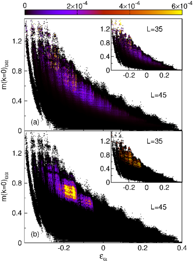
Figure 7: (Color online) Density plots of the coarse-grained weights of energy eigenstates in (a) the DE and (b) the GME as a function of the expectation value of $m(k=0)$ and the eigenstate energy per site $\varepsilon_{\alpha}=E_{\alpha}/L$, for quenches of HCBs to the delocalized regime. Results are shown for systems with $L=45$ (main panel) and $L=35$ (insets). The width of the windows used in the coarse graining is $5\times 10^{-3}$ in $m(k=0)$ and $2\times 10^{-3}$ in $\varepsilon$.

We now present results that indicate that this mechanism is indeed the explanation why the GGE provides an accurate description of HCB observables after relaxation in quenches to the delocalized phase. In Fig. 7, we show density plots of the coarse-grained weights with which eigenstates contribute to the DE [Fig. 7(a)] and to the GME [Fig. 7(b)] for delocalized HCB systems with $L=45$ (main panels) and $L=35$ (insets). We see that in both ensembles, as the system size increases, weight becomes increasingly concentrated in eigenstates with $-0.2<\varepsilon_{\alpha}\equiv E_{\alpha}/L<-0.1$ (though more clearly in the GME than in the DE). Moreover, the expectation values of $\hat{m}(k=0)$ in these most highly weighted eigenstates are narrowly distributed compared to the full range of expectation values of all eigenstates within the same energy range. Furthermore, it is remarkable that the expectation values of $\hat{m}(k=0)$ in the dominant states of the two ensembles are similar to each other, and that this agreement is seen to improve with increasing system size.

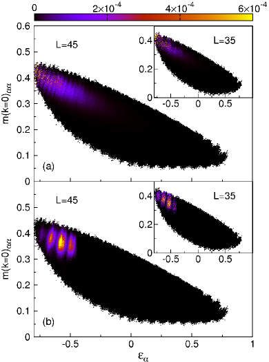
Figure 8: (Color online) Density plots of the coarse-grained weights of energy eigenstates in (a) the DE and (b) the GME as a function of $m(k=0)$ and the eigenstate energy per site $\varepsilon_{\alpha}=E_{\alpha}/L$, for quenches of HCBs to the localized regime. Results are shown for systems with $L=45$ (main panel) and $L=35$ (insets). The width of the windows used in the coarse graining is $10^{-3}$ in $m(k=0)$ and $4\times 10^{-3}$ in $\varepsilon$.

In Fig. 8 we present the corresponding results for quenches to the localized phase. We observe qualitative differences between the distributions of weights in the DE and in the GME: the former are spread relatively smoothly over energies $\varepsilon_{\alpha}<-0.3$ [Fig. 8(a)], whereas the latter tend to concentrate in several distinct energy bands [Fig. 8(b)]. Moreover, in the DE the weights tend to increase as $\varepsilon_{\alpha}$ decreases, corresponding to larger values of the expectation of $\hat{m}(k=0)$, whereas in the GME the weight distribution is more strongly concentrated in eigenstates with higher values of $\varepsilon_{\alpha}$, and smaller values of the zero-momentum expectation values. This suggests that the dominant eigenstates in each of the two ensembles do not yield similar momentum distribution functions, implying the failure of generalized eigenstate thermalization in the localized phase, similar to the failure of eigenstate thermalization in nonintegrable systems in the presence of localization Khatami et al. (2012).

In what follows, we explore in more detail the properties of the eigenstate expectation values of particular observables of interest for SFs and HCBs, and their dependence on the system size.

IV.1 Quenches to the delocalized regime

We start by studying the behavior of the density profiles in the many-body eigenstates of the SF and HCB Hamiltonians. The density profiles of SFs and HCBs are identical, and, by construction, the predictions of the GGE for the expectation value of this observable are the same as those of the DE.

In Fig. 9(a), we show the density profiles after a quench to the delocalized regime as predicted by the DE, the GME, and the ME. The agreement between DE and GME is excellent, as evidenced by the small values of $\Delta n^{\textrm{GME-DE}}$ in Fig. 9(b). The latter quantity is seen to decrease with increasing system size indicating that the DE and GME predictions will agree in the thermodynamic limit. On the other hand, in Fig. 9(a), large differences can be seen between the outcomes of DE and ME calculations for the density profiles, which leads to large values of $\Delta n^{\textrm{ME-DE}}$ as depicted in the inset in Fig. 9(b). The results in the inset suggest that $\Delta n^{\textrm{ME-DE}}$ saturates to a finite value with increasing $L$, which would be consistent with the results of Ref. Gramsch and Rigol (2012), where it was shown that the outcomes of the relaxation dynamics for this observable failed to approach the predictions of the grand-canonical ensemble with increasing system size (for systems up to 20 times larger than those considered here).

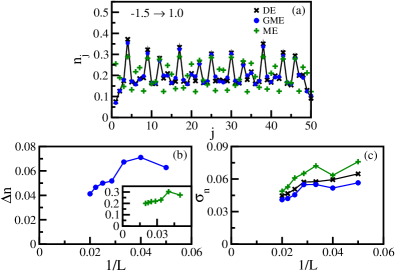
Figure 9: (Color online) (a) Density profiles ($L=50$), (b) $\Delta n^{\textrm{stat-DE}}$, and (c) $\sigma_{n}^{\textrm{stat}}$ in quenches to the delocalized regime, $\lambda_{I}=-1.5\rightarrow\lambda_{F}=1.0$. In (b), the main panel depicts $\Delta n^{\textrm{GME-DE}}$, while the inset depicts $\Delta n^{\textrm{ME-DE}}$. The legends for the ensembles considered are the same in all panels and are reported in (a). The values of $\delta_{\textrm{GME}}$ and $\delta_{\textrm{ME}}$ are the same for all $L$’s and are equal to the ones in Fig. 6.

Figure 9(c) shows the scaling of the average variance of the site occupations in the DE, the GME, and the ME with $L$. In all ensembles, this variance is of a similar small magnitude, and decreases with increasing system size. However, our results are not conclusive as to whether the variance (in any of the ensembles) vanishes or saturates to a finite value in the thermodynamic limit. Inasmuch as we understand thermalization in an isolated system to result from eigenstate thermalization, the fact that this observable does not thermalize Gramsch and Rigol (2012) implies that eigenstate thermalization does not occur in this system. Given that the predictions of the GGE and GME for $n_{j}$ agree with those of the DE, it remains to be clarified in future studies whether the generalized eigenstate thermalization scenario is valid for this observable or not.

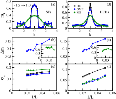
Figure 10: (Color online) [(a),(d)] Momentum distribution functions ($L=50$), [(b),(e)] $\Delta m^{\textrm{stat-DE}}$, and [(c),(f)] $\sigma_{m}^{\textrm{stat}}$, for SFs (left column) and HCBs (right column), in quenches to the delocalized regime, $\lambda_{I}=-1.5\rightarrow\lambda_{F}=1.0$. In [(b),(e)], the main panels depict $\Delta m^{\textrm{GME-DE}}$, while the insets depict $\Delta m^{\textrm{ME-DE}}$. The legends for the ensembles considered are the same in all panels and are reported in (d). The values of $\delta_{\textrm{GME}}$ and $\delta_{\textrm{ME}}$ are the same for all $L$’s and are equal to the ones in Fig. 6.

In Fig. 10, we present a study equivalent to the one in Fig. 9, but for the momentum distributions of SFs and HCBs. The first feature that is apparent in Figs. 10(a) and 10(d) is the contrast between the shapes of the momentum distributions of SFs and HCBs. For small values of $k$, the former resembles a Fermi sea and the latter resembles a bosonic system, both systems at finite but low temperature Rigol (2005). However, the high occupation of $m^{f}_{k}$ and $m^{b}_{k}$ in the tails makes it evident that the systems are not in thermal equilibrium, as can be seen by comparing them to the predictions of the ME. By contrast, the GME predictions for the momentum distributions closely agree with the DE results. This can be seen more clearly in Figs. 10(b) and 10(e), which show that the differences between the GME and the DE predictions are small and decrease with increasing system size. The insets to the same panels show that $\Delta m^{\textrm{ME-DE}}$ is several times larger than $\Delta m^{\textrm{GME-DE}}$ for the system sizes studied, and that the fermionic $\Delta m^{\textrm{ME-DE}}$ has a tendency to saturate to a finite value as $L\rightarrow\infty$, though the behavior of $\Delta m^{\textrm{ME-DE}}$ for HCBs is less clear.

The results for the scaling of $\sigma_{m}^{\textrm{stat}}$ with increasing system size [Figs. 10(c) and 10(f)] make apparent a fundamental difference between the behavior of eigenstate expectation values of $\hat{m}^{f}_{k}$ and $\hat{m}^{b}_{k}$. In each ensemble, $\sigma_{m}^{\textrm{stat}}$ for SFs [Fig. 10(c)] is seen to be larger than the corresponding variance $\sigma_{m}^{\textrm{stat}}$ for HCBs [Fig. 10(f)], and the former appears to saturate to a finite value (more obviously in the ME than in the DE or GME), while the latter appears to vanish (more clearly in the GME and ME than in the DE), in the thermodynamic limit. This makes evident that localization of the single-particle fermionic eigenstates in momentum space has a clear consequence on the behavior of $m^{f}_{k}$ in the many-body eigenstates, for which $\sigma_{m}^{\textrm{stat}}$ may be finite in the thermodynamic limit. By contrast, such a localization phenomenon in the single-particle basis of the SF model appears not to have any effect on the many-body eigenstate expectation values of the momentum distribution of the corresponding HCBs, for which generalized eigenstate thermalization may take place as $\sigma_{m}^{\textrm{stat}}$ appears to vanish for all ensembles, and $\langle\hat{m}^{b}_{k}\rangle_{\textrm{DE}}=\langle\hat{m}^{b}_{k}\rangle_{\textrm{GME}}$ Gramsch and Rigol (2012). Again, we stress that even if the bosonic $\sigma_{m}^{\textrm{ME}}$ does vanish in the thermodynamic limit, we can infer that eigenstate thermalization does not occur for $m^{b}_{k}$ from the failure of this observable to thermalize Gramsch and Rigol (2012).

IV.2 Quenches to the localized regime

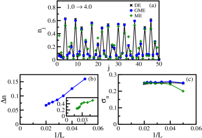
Figure 11: (Color online) (a) Density profiles ($L=50$), (b) $\Delta n^{\textrm{stat-DE}}$, and (c) $\sigma_{n}^{\textrm{stat}}$ in quenches to the localized regime, $\lambda_{I}=1.0\rightarrow\lambda_{F}=4.0$. In (b), the main panel depicts $\Delta n^{\textrm{GME-DE}}$, while the inset depicts $\Delta n^{\textrm{ME-DE}}$. The legends for the ensembles considered are the same in all panels and are reported in (a). The values of $\delta_{\textrm{GME}}$ and $\delta_{\textrm{ME}}$ are the same for all $L$’s and are equal to the ones in Fig. 6.

Density profiles obtained within the DE, GME, and ME after a quench to the localized regime are shown in Fig. 11(a), and the scalings of $\Delta n^{\textrm{GME-DE}}$ ($\Delta n^{\textrm{ME-DE}}$) with increasing system size are reported in the main panel (inset) in Fig. 11(b). Despite the fact that the site occupations fluctuate from site to site much more in Fig. 11(a) than in Fig. 9(a), the GME results still closely agree with those of the DE, while the ME results do not. The scaling of $\Delta n^{\textrm{GME-DE}}$ with increasing system size suggests that the differences between the predictions of the GME and the DE will vanish in the thermodynamic limit. The results for $\Delta n^{\textrm{ME-DE}}$ are less conclusive, although the values of this quantity obtained for the largest system sizes suggest a possibly tendency toward saturation.

A clear difference between the behavior of the site occupations in the localized and delocalized regimes is seen in the fact that the variance of the eigenstate expectation values of this observable saturates in all three ensembles to a finite value in the former [Fig. 11(c)], whereas our results suggest that it vanishes in the latter [Fig. 9(c)], as the system size is increased. The saturation observed in Fig. 11(c) is a clear consequence of localization of the single-particle eigenstates in real space for $\lambda>\lambda_{c}$. Finite values of the fermionic $\sigma_{m}^{\textrm{ME}}$ in the delocalized regime and of $\sigma_{n}^{\textrm{ME}}$ in the localized one are physically relevant examples of the failure of the variance of few-body observables in the many-body eigenstates that constitute the ME to vanish in the thermodynamic limit, contrary to what is generally expected to occur for few-body observables Biroli et al. (2010).

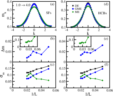
Figure 12: (Color online) [(a),(d)] Momentum distribution functions ($L=50$), [(b),(e)] $\Delta m^{\textrm{stat-DE}}$, and [(c),(f)] $\sigma_{m}^{\textrm{stat}}$, for SFs (left column) and HCBs (right column), in quenches to the localized regime, $\lambda_{I}=1.0\rightarrow\lambda_{F}=4.0$. In [(b),(e)], the main panels depict $\Delta m^{\textrm{GME-DE}}$, while the insets depict $\Delta m^{\textrm{ME-DE}}$. The legends for the ensembles considered are the same in all panels and are reported in (d). The values of $\delta_{\textrm{GME}}$ and $\delta_{\textrm{ME}}$ are the same for all $L$’s and are equal to the ones in Fig. 6.

In Figs. 12(a) and 12(d), we show the momentum distribution functions of SFs and HCBs in the DE, the GME, and the ME after a quench to the localized regime. In each ensemble, the results for SFs and HCBs are barely distinguishable from each other, which we might intuitively attribute to localization undermining the particle statistics. As in the quenches to the delocalized regime, the GME results closely follow those of the DE, and the main panels in Figs. 12(b) and 12(e) indicate that $\Delta m^{\textrm{GME-DE}}$ decreases with increasing system size. Whereas we expect $\Delta m^{\textrm{GME-DE}}$ to vanish for SFs in the thermodynamic limit (as the DE and GGE predictions coincide for all one-body fermionic observables), for HCBs we expect it to converge to a small but finite value, because of the failure of the GGE to describe the time averages of the HCB momentum distribution function observed in Ref. Gramsch and Rigol (2012). In Figs. 12(a) and 12(d), the ME results for the momentum distributions are clearly distinct from those of the DE, and that difference is expected to remain in the thermodynamic limit both for SFs and HCBs, as suggested by the scaling of $\Delta m^{\textrm{ME-DE}}$ in the insets in Figs. 12(b) and 12(e).

Results for the scaling of $\sigma_{m}^{\textrm{stat}}$ with increasing system size are presented in Figs. 12(c) and 12(f), for SFs and HCBs, respectively. Once again, the results for the two-particle species are very similar to each other. They are particularly inconclusive for $\sigma_{m}^{\textrm{ME}}$, which is seen to increase with increasing system size for all systems except the two largest ones, for which it is seen to decrease. On the other hand, $\sigma_{m}^{\textrm{DE}}$ and $\sigma_{m}^{\textrm{GME}}$ decrease for all system sizes, though the results for the largest two system sizes suggest that they may saturate. This leaves open the question of whether $\sigma_{m}^{\textrm{stat}}$ vanishes in the thermodynamic limit or whether it remains finite. What is clear from the fact that both the grand-canonical ensemble and the GGE fail to describe $m^{b}_{k}$ after relaxation Gramsch and Rigol (2012) is that neither eigenstate thermalization nor generalized eigenstate thermalization take place in the HCB system in this regime.

IV.3 Quenches to the critical point

For completeness, we present here results for the ensemble expectation values of observables in quenches to the critical point. We note that in light of the results of Sec. III and Ref. Gramsch and Rigol (2012), we might expect the critical regime to be particularly sensitive to finite-size effects.

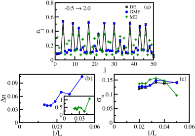
Figure 13: (Color online) (a) Density profiles ($L=50$), (b) $\Delta n^{\textrm{stat-DE}}$, and (c) $\sigma_{n}^{\textrm{stat}}$ in quenches to the critical point, $\lambda_{I}=-0.5\rightarrow\lambda_{F}=2.0$. In (b), the main panel depicts $\Delta n^{\textrm{GME-DE}}$, while the inset depicts $\Delta n^{\textrm{ME-DE}}$. The legends for the ensembles considered are the same in all panels and are reported in (a). The values of $\delta_{\textrm{GME}}$ and $\delta_{\textrm{ME}}$ are the same for all $L$’s and are equal to the ones in Fig. 6.

In Fig. 13 we present results for the density profiles, which are intermediate between those observed for quenches to the delocalized and localized phases, as expected due to the small finite sizes of the lattice systems studied. In particular, the average variance $\sigma_{n}^{\textrm{stat}}$ decreases with increasing system size but has a tendency to saturate, so much larger system sizes will be needed to resolve whether it vanishes in the thermodynamic limit (as it may in quenches to the delocalized phase) or whether it remains finite (as expected from the observed behavior in quenches to the localized phase).

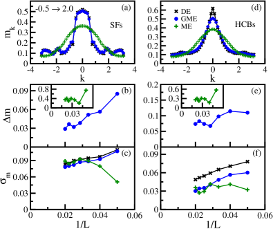
Figure 14: (Color online) [(a),(d)] Momentum distribution functions ($L=50$), [(b),(e)] $\Delta m^{\textrm{stat-DE}}$, and [(c),(f)] $\sigma_{m}^{\textrm{stat}}$, for SFs (left column) and HCBs (right column), in quenches to the critical point, $\lambda_{I}=-0.5\rightarrow\lambda_{F}=2.0$. In [(b),(e)], the main panels depict $\Delta m^{\textrm{GME-DE}}$, while the insets depict $\Delta m^{\textrm{ME-DE}}$. The legends for the ensembles considered are the same in all panels and are reported in (d). The values of $\delta_{\textrm{GME}}$ and $\delta_{\textrm{ME}}$ are the same for all $L$’s and are equal to the ones in Fig. 6.

Figure 14 shows results for the momentum distribution functions of SFs (left columns) and HCBs (right columns). They are also intermediate between those obtained in the delocalized and localized regimes. The average variance $\sigma_{m}^{\textrm{stat}}$ is larger for SFs than for HCBs, as in the delocalized phase. It can also be seen to decrease with increasing system size (as it does in the localized phase), but has a tendency to saturate (as it does in the delocalized phase), so results for much larger system sizes will be needed to resolve whether it vanishes or remains finite in the thermodynamic limit.

V summary

We have studied the dynamics of the momentum distribution function of noninteracting spinless fermions following quenches to the delocalized, localized, and critical regimes of a quasiperiodic lattice system. We found that although the time-averaged value of this observable agrees exactly with the predictions of the GGE in all three regimes, it does not exhibit relaxation after a quench in the delocalized phase. This is complementary to the failure of the on-site density of hard-core bosons (and therefore the noninteracting fermion system considered here) to equilibrate in the localized regime that was previously observed in Ref. Gramsch and Rigol (2012). These behaviors can be understood in terms of localization of the single-particle eigenstates of the fermion model, in momentum space for the delocalized regime, and in real space for the localized regime, as discussed in Refs. Cazalilla et al. (2012); Ziraldo et al. (2012); Ziraldo and Santoro (2013). This analysis also helps us understand the previously observed failure of the GGE to describe the momentum distribution functions of HCBs after relaxation in the localized regime Gramsch and Rigol (2012) as a consequence of nonvanishing time fluctuations of one-particle fermionic correlations that persist in the thermodynamic limit.

We found that in the delocalized and localized regimes, the SF observables that do exhibit relaxation to the GGE—the density in the former case, and the momentum distribution function in the latter—do so in a manner consistent with the Gaussian equilibration picture of Campos Venuti and Zanardi Campos Venuti and Zanardi (2013). In quenches to the critical point of the Aubry-André model, we observed that both the density and the momentum distribution function of SFs exhibit equilibration to the GGE, but that the decay of the time fluctuations of these quantities with increasing system size is slower than that predicted by the conjecture of Ref. Campos Venuti and Zanardi (2013).

We also studied the expectation values of one-body observables in the many-body eigenstates of the SF and HCB Hamiltonians, comparing results for the diagonal, microcanonical, and generalized microcanonical ensembles. We found a clear distinction between the predictions of the ME for the expectation values and those of the GME. The differences between the expectation values in the former ensemble and the DE were consistently larger (and were in fact greater than 10% in all cases except for the momentum distributions in quenches to the localized phase) and indications were found that these differences approach nonzero values as the system size is increased toward the thermodynamic limit. The predictions of the GME were found to be much closer to those of the DE and, for the system sizes studied, the differences between the expectation values in these two ensembles were observed in most cases to decrease with increasing system size.

Our study indicates that the single-particle localization—in momentum space in the delocalized regime and in real space in the localized regime—that precludes relaxation of the corresponding observables to the GGE also leads to finite thermodynamic-limit variances of momentum and site occupations, respectively, in the many-body eigenstates of the SF Hamiltonian. By contrast, the failure of the GGE to describe the momentum distribution of HCBs after relaxation in the localized phase was not found to be associated with any corresponding saturation of the variance of momentum occupations in eigenstates of the HCB Hamiltonian with increasing system size.

Because of finite-size effects, we did not find clear indications of the behavior of the maximum differences between expectation values of the density and momentum distributions in distinct eigenstates contributing to the various ensembles as the system size is increased. It would be particularly important to understand whether the values of observables in the individual eigenstates constituting the GME approach their average values in this ensemble with increasing system size, in order to clarify whether generalized eigenstate thermalization occurs in the delocalized regime—which would explain why the GGE works there for describing the momentum distribution functions of HCBs after relaxation—and whether generalized eigenstate thermalization fails (as we expect) in the localized regime, where the GGE fails. It would also be interesting to see how the addition of nearest neighbor interactions Tezuka and García-García (2010, 2012); Iyer et al. (2013), which break integrability, modify our findings for both SFs and HCBs.