Efficient Wireless Security
Through Jamming, Coding and Routing

Abstract

There is a rich recent literature on how to assist secure communication between a single transmitter and receiver at the physical layer of wireless networks through techniques such as cooperative jamming. In this paper, we consider how these single-hop physical layer security techniques can be extended to multi-hop wireless networks and show how to augment physical layer security techniques with higher layer network mechanisms such as coding and routing. Specifically, we consider the secure minimum energy routing problem, in which the objective is to compute a minimum energy path between two network nodes subject to constraints on the end-to-end communication secrecy and goodput over the path. This problem is formulated as a constrained optimization of transmission power and link selection, which is proved to be NP-hard. Nevertheless, we show that efficient algorithms exist to compute both exact and approximate solutions for the problem. In particular, we develop an exact solution of pseudo-polynomial complexity, as well as an $\epsilon$-optimal approximation of polynomial complexity. Simulation results are also provided to show the utility of our algorithms and quantify their energy savings compared to a combination of (standard) security-agnostic minimum energy routing and physical layer security. In the simulated scenarios, we observe that, by jointly optimizing link selection at the network layer and cooperative jamming at the physical layer, our algorithms reduce the network energy consumption by half.

I Introduction

Protecting the secrecy of user messages has become a major concern in modern communication networks. Due to the propagation properties of the wireless medium, wireless networks can potentially make the problem more challenging by allowing an eavesdropper to have relatively easy access to the transmitted message if countermeasures are not employed. Our goal is to provide everlasting security in this wireless environment; that is, we will consider methods that will prevent an eavesdropper from ever decoding a transmitted message - even if the eavesdropper has the capability to record the signal and attempt decryption over many years (or decades). There are two different classes of security techniques of interest here: cryptographic approaches based on computational complexity, and information-theoretic approaches that attempt to obtain perfect secrecy. Both have advantages and disadvantages for the desired everlasting security in the wireless environment.

The traditional solution to providing security in a wireless environment is the cryptographic approach: assume that the eavesdropper will get the transmitted signal without distortion, but the desired recipient who shares a key with the transmitter is able to decode the message easily, while the eavesdropper lacking the key must solve a hard problem that is beyond her/his computational capabilities [1]. Since the eavesdropper is assumed to get the transmitted signal without distortion, cryptography addresses the key challenge in the wireless environment of thwarting an eavesdropper very near the transmitter. However, such an approach faces the concern that the eavesdropper can store the signal, and, then, with later advances in computational capabilities or by breaking the encryption scheme, obtain the message. The desire for everlasting security then motivates adding countermeasures at the physical layer that inhibit even the recording of the encrypted message by the eavesdropper that combine with cryptography to facilitate a defense-in-depth approach [2].

In the information-theoretic approach to obtain perfect secrecy [3], the goal is to guarantee that the eavesdroppers can never extract information from the message, regardless of their computational capability. Wyner [4] and succeeding authors [5, 6] showed that perfect secrecy is possible if the channel conditions between the transmitter and receiver were favorable relative to the channel conditions between the transmitter and eavesdropper. In this so-called wiretap channel, perfect secrecy at a positive rate with no pre-shared key is possible [4]. This clearly satisfies the requirement for everlasting secrecy, but it relies on favorable channel conditions that are difficult (if not impossible) to guarantee in a wireless environment. Hence, information-theoretic secrecy requires a network design which inhibits reception at the eavesdropper while supporting reception at the desired recipient.

Our work supports both a cryptographic (computational) approach or information-theoretic approach. Per above, it is advantageous in either case to seek or create conditions so as to inconvenience reception at eavesdropper(s) while facilitating communication of the legitimate system nodes. This has been actively considered in the literature on the physical layer of wireless networks over the last decade, with approaches based on both opportunism [7, 8] and active channel manipulation [9, 10] being employed. Most of these works have arisen in the information-theoretic community and considered small networks consisting of a source, destination, eavesdropper, and perhaps a relay node(s) [8, 9, 10, 11, 12, 13]. More recently, there has been the active consideration of large networks with the introduction of the secrecy graph to consider secure connectivity [14, 15, 16] and a number of approaches to throughput scaling versus security tradeoffs [17, 18, 19]. Hence, whereas there has been a significant consideration of small single- and two-hop networks and asymptotically large multi-hop networks, there has been almost no consideration of the practical multi-hop networks that lie between those two extremes. It is this large and important gap that this paper fills.

Consider a network where system nodes communicate with each other wirelessly, possibly over multiple hops, such as in wireless mesh networks and ad hoc networks. A set of eavesdroppers try to passively listen to communications among legitimate network nodes. To prevent the eavesdroppers from successfully capturing communications between legitimate nodes, mechanisms to thwart such are employed at the physical layer of the network. Two nodes that wish to communicate securely may need to do so over multiple hops in order to thwart eavesdroppers or simply because the nodes are not within the reach of each other. While we make no argument about the optimality or practicality of any specific physical layer security mechanism, for the sake of concreteness, we focus on cooperative jamming, which has received considerable attention  [9, 10, 11, 12, 13, 20]. In cooperative jamming, whenever a node transmits a message, a number of cooperative nodes, called jammers, help the node conceal its message by transmitting a carefully chosen signal to raise the background noise level and degrade the eavesdropping channels. Because our general philosophy applies to any physical layer approach, the framework can be extended to include other forms of physical layer security. However, some of the attractive features of cooperative jamming that motivated us to study this technique include:

1. Opportunistic techniques [7, 8] that exploit the time-varying wireless channel may suffer from excessive delays depending on the rate of channel fluctuations. For applications that require security without an excessive delay, active channel manipulation such as cooperative jamming should be adopted. The price to be paid, in this case, is the increased interference due to jamming.

2. Multi-antenna systems can also be used to jam eavesdroppers [21, 9]. However, the use of multiple antennas on every wireless device may not be feasible due to cost and size (e.g., wireless sensors). Cooperative jamming is a distributed alternative to multi-antenna systems.

3. Node cooperation, while requiring a more complex physical layer, is incorporated in commercial wireless technologies such as LTE. Thus, we envision that cooperative jamming can be implemented in practice, as was demonstrated in a limited form (single jammer) in [22].

4. Anonymous wireless communication is a challenging problem. Cooperative jamming can potentially be utilized for wireless anonymous communication, as it creates confusion for wireless localization techniques [23].

In this general case, the main questions are: (1) how to choose the intermediate nodes that form a multi-hop path from the source node to the destination node, and (2) how to configure each hop at the physical layer with respect to the security and throughput constraints of the path. Specifically, the problem we consider in this paper is how to find a minimum cost path between a source and destination node in the network, while guaranteeing a pre-specified lower bound on the end-to-end secrecy and goodput of the path. The cost of a path can be defined in terms of various system parameters. In a wireless network, transmission power is a critical factor affecting the throughput and lifetime of the network. While increasing the transmission power results in increased link throughput, excessive power actually results in high levels of interference, hence reducing the network throughput due to inefficient spacial reuse. With cooperative jamming at the physical layer, transmission power is even more important due to the additional interference caused by jamming signals if they need to be employed. Thus, in this work, we consider the amount of end-to-end transmission power as the cost of a path with the objective of finding secure paths that consume the least amount of energy. In turn, such paths, by minimizing interference in the network, result in higher throughput. Note that solutions employing power only at the nodes transmitting the messages (and no cooperative jamming) are part of the space over which the optimization will be performed; thus, if it is more efficient to not employ cooperative jamming, such a solution will be revealed by our algorithms.

While it might seem that physical layer security techniques can be extended to multi-hop networks by implementing them on a hop-by-hop basis, in general, such extensions sacrifice performance or are not feasible. The eavesdropping probability on a link is a function of the power allocation on that link. A hop-by-hop implementation is unable to determine the optimal eavesdropping probability and consequently power allocation for each link in order to satisfy the end-to-end constraints (i.e., the chicken-egg problem). Moreover, a hop-by-hop approach overlaid on a shortest path routing algorithm might pay an enormous penalty to mitigate eavesdroppers on some links (e.g., by routing through a node with one or more links, that, because of system geometry, are very vulnerable to nearby eavesdroppers). A routing algorithm that is designed in conjunction with physical layer security can selectively employ links that are easier to secure when it is power-efficient to do so and, in such a way, minimize the impact of the security constraint on end-to-end throughput.

Our main contributions can be summarized as follows:

• We formulate the secure minimum energy routing problem with end-to-end security and goodput constraints as a constrained optimization of transmission power at the physical layer and link selection at the network layer.

• We prove that the secure minimum energy routing problem is NP-hard, and develop exact and $\epsilon$-approximate solutions of, respectively, pseudo-polynomial and fully-polynomial time complexity for the problem.

• We show how cooperative jamming can be used to establish a secure link between two nodes in the presence of multiple eavesdroppers or probabilistic information about potential eavesdropping locations by utilizing random linear coding at the network layer.

• We provide simulation results that demonstrate the significant energy savings of our algorithms compared to the combination of security-agnostic minimum energy routing and physical layer security.

The rest of the paper is organized as follows. Our system model is described in Section II. The optimal link and path cost are analyzed in Sections III and IV. Our routing algorithms are presented in Section V. Simulation results are discussed in Section VI. Section VII presents an overview of some related work, while Section VIII concludes the paper.

II System Model and Assumptions

Consider a wireless network with arbitrarily distributed nodes. We assume that each node (legitimate or eavesdropper) is equipped with a single omni-directional antenna. A $K$-hop route $\Pi$ between a source and a destination in the network is a sequence of $K$ links connecting the source to the destination. We use the notation $\Pi=\langle\ell_{1},\ldots,\ell_{K}\rangle$ to refer to a route that is formed by $K$ links $\ell_{1}$ to $\ell_{K}$. A link $\ell_{k}\in\Pi$ is formed between two nodes $S_{k}$ and $D_{k}$ on route $\Pi$. We assume that every link $\ell_{k}$ is exposed to a set of (potential) eavesdroppers denoted by $\mathcal{E}_{k}$. Whenever $S_{k}$ transmits a message to $D_{k}$, a set of trusted nodes, called jammers, cooperate with $S_{k}$ to conceal its message from the eavesdroppers in $\mathcal{E}_{k}$ by jamming $S_{k}$’s signal at the eavesdroppers. The set of the jammers cooperating with $S_{k}$ to conceal its transmissions from $\mathcal{E}_{k}$ is denoted by $\mathcal{J}_{k}=\left\{J_{1}\ldots,J_{|\mathcal{J}_{k}|}\right\}$, where $|\mathcal{A}|$ denotes the cardinality of set $\mathcal{A}$. The set of jammers is potentially different for different links. Throughout the paper, we use the notation $(S_{k},D_{k},\mathcal{E}_{k},\mathcal{J}_{k})$ to identify link $\ell_{k}$.

In the following subsections, we describe the models considered in this paper for the wireless channel, eavesdroppers, physical-layer security and end-to-end routing. For notational simplicity, we may drop the link index $k$ whenever there is no ambiguity.

II-A Wireless Channel Model

Consider the discrete-time equivalent model for a transmission from node $S$ to node $D$. Let $x_{S}$ be the normalized (unit-power) symbol stream to be transmitted by $S$, and let $y_{D}$ be the received signal at node $D$. We assume that transmitter $S$ is able to control its power $P_{S}$ in arbitrarily small steps, up to some maximum power $P_{\mathrm{max}}$. Let $n_{D}$ denote the receiver noise at $D$, where $n_{D}$ is assumed to be a complex Gaussian random variable with $\mathbb{E}\left[|n_{D}|^{2}\right]=N_{0}$. The received signal at $D$ is expressed as

$$y_{D}=\sqrt{P_{S}}\,h_{S,D}\,x_{S}+n_{D},$$ (1)

where $h_{S,D}$ is the complex channel gain between $S$ and $D$. The channel gain is modeled as $h_{S,D}=|h_{S,D}|e^{\theta_{S,D}}$, where $|h_{S,D}|$ is the channel gain magnitude and $\theta_{S,D}$ is the uniform phase. We assume a non line-of-sight environment, implying that $|h_{S,D}|$ has a Rayleigh distribution, and that $\mathbb{E}[|h_{S,D}|^{2}]=1/d_{S,D}^{\alpha}$, where $d_{S,D}$ is the distance between nodes $S$ and $D$, and $\alpha$ is the path-loss exponent (typically between $2$ and $6$). This is the standard narrowband fading channel model employed in the physical layer literature [24, 25].

II-B Adversary Model

We limit our attention to passive eavesdroppers as in prior work [9, 10, 11, 12, 13, 20]. Although there are other forms of adversarial behavior, their consideration is beyond the scope of this paper.

While the literature on physical layer security often assumes not only eavesdropper locations but also either perfect (e.g., [10]) or imperfect (e.g., [20]) knowledge at the transmitters and jammers of the complex channel gains of the eavesdropping channels (i.e., availability of instantaneous eavesdropper channel state information (CSI)), we consider the more realistic scenario, in which CSI for eavesdropping channels is not available. In addition, our model requires only the knowledge of potential eavesdropping locations in the network, yet we show that it provides guaranteed security by employing coding in conjunction with cooperative jamming.

Specifically, we assume that each link $\ell_{k}$ is subject to potential eavesdropping from a set of locations denoted by $\mathcal{E}_{k}=\left\{E_{1},\ldots,E_{|\mathcal{E}_{k}|}\right\}$, where the probability of eavesdropping from location $E_{i}$ is given by $p(E_{i})$ for $0\leq p(E_{i})\leq 1$. This is a considerably general model that can be used to represent a wide range of eavesdropping scenarios. For example, setting all $p(E_{i})$’s to $1$ for a link models multiple eavesdroppers for that link. Other examples include, for example, military scenarios where the locations of enemy installations are known, or wireless networks where a malicious user(s) has been detected. In general, for any given link, there is only a limited region around the link that can be exploited for eavesdropping. By dividing the effective eavesdropping region to a few smaller areas [26], one can compute the most effective eavesdropping location within each area, and consequently, construct the set of eavesdropping locations for that link.

II-C Physical Layer Security Model

Consider a secure link formed between source $S$ and receiver $D$ with the help of jammers $\mathcal{J}$. For the moment, we assume that cooperative jamming is implemented at the physical layer to deal with a single eavesdropper $E$ located at a fixed position. Later, in Section III, we show how this physical layer primitive can be used to provide security against multiple eavesdroppers or unknown eavesdropping locations.

When node $S$ transmits a message, there are multiple ways in which cooperative jamming by system nodes can be exploited, ranging from relatively simple noncoherent techniques to sophisticated beamforming techniques [27]. Since the implementation of beamforming in other contexts, with the same challenges of synchronization in the wireless environment, is advancing rapidly [28, 29], we assume that the jammers cooperatively beamform a common artificial noise signal $z$ to the receiver in such a way that their signals cancel out at the receiver [30]. The noise signal $z$ is transmitted in the null space of the channel vector $\mathbf{h}_{D}=[h_{J_{1},D},h_{J_{2},D},\ldots,h_{J_{|\mathcal{J}|},D}]^{\mathrm{T}}$ where, $h_{J_{i},D}$ denotes the channel gain between jammer $J_{i}$ and destination $D$ and $\mathbf{A}^{\mathrm{T}}$ denotes the conjugate transpose of vector $\mathbf{A}$. Thus, the signal transmitted by the jammers can be expressed as $\mathbf{s}_{J}=\mathbf{h}_{D}^{\perp}\,z$, where $\mathbf{h}_{D}^{\perp}$ is a vector chosen in the null space of $\mathbf{h}_{D}$. It follows that the total transmission power of the jammers is given by $P_{J}=\parallel\mathbf{h}_{D}^{\perp}\parallel^{2}$. Assuming that the source node transmits with power $P_{S}$, the signals received at the destination and the eavesdropper are given by

$$\begin{split}y_{D}&=\sqrt{P_{S}}\,h_{S,D}\,x_{S}+n_{D},\\ y_{E}&=\sqrt{P_{S}}\,h_{S,E}\,x_{S}+\mathbf{h}_{E}^{\mathrm{T}}\mathbf{h}_{D}^{\perp}z+n_{E},\end{split}$$ (2)

where, $\mathbf{h}_{E}=[h_{J_{1},E},h_{J_{2},E},\ldots,h_{J_{|\mathcal{J}|},E}]^{\mathrm{T}}$ represents the channel gain vector between the jammers and the eavesdropper, and $n_{D}$ and $n_{E}$ denote the complex Gaussian noise at the destination and eavesdropper, respectively, with $\mathbb{E}\left[|n_{D}|^{2}\right]=\mathbb{E}\left[|n_{E}|^{2}\right]=N_{0}$.

Although the jammers try to prevent the eavesdropper from successfully receiving the message, there is still some probability that the eavesdropper actually obtains the message due to the fact that the channel to the eavesdropper is unknown in our model, i.e., $\mathbf{h}_{E}$ and $h_{S,E}$ are unknown. Recalling that the signal-to-interference-plus-noise ratio ($\mathrm{SINR}$) at the destination is controlled via power control, let $\gamma_{E}$ denote the minimum required $\mathrm{SINR}$ at the eavesdropper in order to violate the security constraints of the protocol (e.g. for the cryptographic case, the $\mathrm{SINR}$ above which the eavesdropper can record a meaningful version of the transmitted signal; in the information-theoretic case, the $\mathrm{SINR}$ above which, for a given wire-tap code, the equivocation does not equal the entropy of the message.) Let $\mathrm{SINR}_{E}$ denote the $\mathrm{SINR}$ at the eavesdropper. We have

$$\begin{split}&\mathbb{P}\left\{\mathrm{SINR}_{E}\geq\gamma_{E}\right\}=\mathbb{P}\left\{\tfrac{P_{S}|h_{S,E}|^{2}}{N_{0}+\mathbf{h}_{E}^{\mathrm{T}}\mathbf{h}_{D}^{\perp}{\mathbf{h}_{D}^{\perp}}^{\mathrm{T}}\mathbf{h}_{E}}\geq\gamma_{E}\right\}\\ &\qquad=\mathbb{E}_{\mathbf{h}_{E}}\left[\mathbb{P}\left\{\frac{P_{S}|h_{S,E}|^{2}}{N_{0}+\mathbf{h}_{E}\mathbf{h}_{D}^{\perp}{\mathbf{h}_{D}^{\perp}}^{\mathrm{T}}\mathbf{h}_{E}^{\mathrm{T}}}\geq\gamma_{E}\Big{|}\,\mathbf{h}_{E}\right\}\right]\\ &\qquad=\mathbb{E}_{\mathbf{h}_{E}}\big{[}e^{-\frac{\gamma_{E}d_{S,E}^{\alpha}}{P_{S}}\mathbf{h}_{E}^{\mathrm{T}}\mathbf{h}_{D}^{\perp}{\mathbf{h}_{D}^{\perp}}^{\mathrm{T}}\mathbf{h}_{E}}\big{]}e^{-\frac{\gamma_{E}N_{0}d_{S,E}^{\alpha}}{P_{S}}},\end{split}$$ (3)

where $\mathbb{E}_{\mathbf{h}_{E}}$ means expectation with respect to channel gain vector $\mathbf{h}_{E}$. Using the results on quadratic forms [31, Eq. 14] to calculate the expectation, it is obtained that ($\mathbf{I}_{N}$ is the identity matrix of size $N$)

$$\begin{split}\mathbb{P}\left\{\mathrm{SINR}_{E}\geq\gamma_{E}\right\}&\leq\frac{e^{-\frac{\gamma_{E}N_{0}d_{S,E}^{\alpha}}{P_{S}}}}{|\mathbf{I}_{N}+\frac{\gamma_{E}d_{S,E}^{\alpha}}{P_{S}}(\sum_{J_{i}\in\mathcal{J}}{\frac{1}{d_{J_{i},E}^{\alpha}}})\mathbf{\mathbf{h}_{D}^{\perp}{\mathbf{h}_{D}^{\perp}}^{\mathrm{T}}}|}\\ &=\frac{e^{-N_{0}\gamma_{E}\frac{d_{S,E}^{\alpha}}{P_{S}}}}{1+\frac{\gamma_{E}d_{S,E}^{\alpha}}{P_{S}}(\sum_{J_{i}\in\mathcal{J}}{\frac{1}{d_{J_{i},E}^{\alpha}}})P_{J}}\,\cdot\end{split}$$ (4)

where the final expression is derived from Sylvester’s determinant theorem:

$$\det(\mathbf{I}_{m}+\mathbf{A}\mathbf{B})=\det(\mathbf{I}_{n}+\mathbf{B}\mathbf{A}),$$

for $\mathbf{A}$ and $\mathbf{B}$ being $m\times n$ and $n\times m$ matrices, respectively, and the fact that $P_{J}={\mathbf{h}_{D}^{\perp}}^{\mathrm{T}}\mathbf{h}_{D}^{\perp}$ (see (31)).

In the remainder of the paper, we use (4) in equality form to compute the eavesdropping probability for a given jamming power $P_{J}$. While this results in a (slightly) conservative power allocation, it is sufficient to satisfy the security requirement of each link.

II-D Routing Model

Consider a $K$-hop route $\Pi=\langle\ell_{1},\ldots,\ell_{K}\rangle$ between a legitimate source and destination in the network. Let $\mathcal{L}$ denote the set of all possible routes between the source and destination. Let $\mathcal{C}(\Pi)$ denote the cost of route $\Pi$, where the cost of a route is defined as the summation of the costs of the links forming the route. With slight abuse of the notation, we use $\mathcal{C}(\ell_{k})$ to denote the cost of link $\ell_{k}$ as well. The secure routing problem is then defined as follows.

SMER: Secure Minimum Energy Routing Problem
Consider a wireless network and a set of eavesdroppers distributed in the network. Given a source and destination, find a minimum energy path $\Pi^{*}$ between the source and destination subject to constraints $\pi$ and $\lambda$ on the end-to-end successful eavesdropping probability and goodput on the path respectively.

Let $\lambda(\Pi)$ and $\lambda(\ell_{k})$ denote, respectively, the goodput of path $\Pi$ and link $\ell_{k}\in\Pi$. Then $\lambda(\Pi)$ can be expressed as

$$\lambda(\Pi)=\min_{\ell_{k}\in\Pi}\lambda(\ell_{k})\,\cdot$$

Since goodput of a link is an increasing function of the transmission power of the transmitter of that link, a necessary condition for minimizing power over the path $\Pi$ is given by $\lambda(\ell_{k})=\lambda$, for all $\ell_{k}\in\Pi$, i.e., all links should just achieve the minimum goodput $\lambda$. Thus, our power allocation scheme (see Section III) establishes links that achieve exactly the minimum required goodput $\lambda$. Consequently, the constraint on the end-to-end goodput is satisfied by any path in the network, and hence does not need to be explicitly considered when solving SMER. As such, SMER can be formally described by the following optimization problem:

$$\begin{split}\Pi^{*}=\,&\displaystyle\arg\min_{\Pi\in\mathcal{L}}\sum_{\ell_{k}\in\Pi}\mathcal{C}(\ell_{k})\\ &s.t.\quad\mathbb{P}\left\{\text{eavesdropping on route $\Pi$}\right\}\leq\pi,\end{split}$$ (5)

for some pre-specified $\pi$ ($0<\pi<1$). The constraint on the route eavesdropping probability in the above optimization problem can be expressed in terms of the eavesdropping probability on individual links $\ell_{k}$ that form the route $\Pi$, as $\prod_{\ell_{k}\in\Pi}(1-\pi_{k})\geq 1-\pi$, where $\pi_{k}$ ($0<\pi_{k}<1$) denotes the successful eavesdropping probability on link $\ell_{k}$. We use the following result to convert the above inequality constraint to an equality constraint in the routing problem (5).

Lemma 1

The cost of route $\Pi$ is a monotonically increasing function of $\prod_{\ell_{k}\in\Pi}(1-\pi_{k})$.

Proof:

Consider a path $\Pi$ between the source and destination nodes. Define the end-to-end secrecy of path $\Pi$, denoted by $\omega(\Pi)$, as follows:

$$\omega(\Pi)=\prod_{\ell_{k}\in\Pi}\omega_{k},$$ (6)

where $\omega_{k}=(1-\pi_{k})$.

First, we show that the link cost $\mathcal{C}(\ell_{k})$ is a monotonically increasing function of the the link secrecy $\omega_{k}$ for every link $\ell_{k}\in\Pi$. Let $P_{S}^{(k)}$ and $P_{J}^{(k)}$ denote the source and jamming powers allocated to the link $\ell_{k}$, respectively. In Section III, we show that: (i) $P_{S}^{(k)}$ is a constant for a given link independent of the link secrecy, and (ii) $P_{J}^{(k)}$ is a function of the link secrecy and is given by

$$P_{J}^{(k)}=c_{k}\cdot\frac{\omega_{k}}{1-\omega_{k}},$$ (7)

where $c_{k}$ is some constant independent of $\omega_{k}$. Thus, for a fixed link $\ell_{k}$, the link cost $\mathcal{C}(\ell_{k})=P_{S}^{(k)}+P_{J}^{(k)}$ depends on $\omega_{k}$ only through the jamming power $P_{J}^{(k)}$. Taking the derivative on the link cost with respect to $\omega_{k}$ results in the following relation:

$$\frac{d}{d\omega_{k}}\,\mathcal{C}(\ell_{k})=c_{k}\cdot\frac{1}{(1-\omega_{k})^{2}}>0,$$ (8)

indicating that the link cost is an increasing function of the link secrecy $\omega_{k}$.

Let $\mathcal{C}^{*}(\Pi)$ and $\mathcal{C}(\Pi)$ denote the optimal cost of the path $\Pi$ computed by solving the optimization problem (14), with equality and inequality constraints, respectively. Furthermore, let $\omega^{*}(\Pi)$ and $\omega(\Pi)$ denote the corresponding end-to-end path secrecies. We present a proof of the lemma based on contradiction by assuming that the optimal path cost with the inequality constraint is less than that with the equality constraint. That is, we assume that

$$\mathcal{C}(\Pi)\leq\mathcal{C}^{*}(\Pi),$$ (9)

while,

$$\omega(\Pi)>\omega^{*}(\Pi)\,\cdot$$ (10)

Next, by manipulating the link secrecy allocation vector $[\omega_{1},\ldots,\omega_{k},\ldots,\omega_{K}]$, we construct a new link secrecy allocation vector that satisfies the equality constraint, while having a cost smaller than $\mathcal{C}^{*}(\Pi)$. To this end, consider some arbitrary link $\ell_{k}$, and replace $\omega_{k}$ by a new $\omega^{\prime}_{k}$ as follows

$$\omega^{\prime}_{k}=\frac{\omega^{*}}{\omega}\cdot\omega_{k}\,\cdot$$ (11)

Since $\omega^{*}<\omega$, it follows that $\omega^{\prime}_{k}<\omega_{k}$. Consequently, the new cost of the link $\ell_{k}$ with link secrecy $\omega^{\prime}_{k}$ is less than $\mathcal{C}(\ell_{k})$, which in turn indicates that the new path cost with secrecy allocation vector $[\omega_{1},\ldots,\omega^{\prime}_{k},\ldots,\omega_{K}]$ is less than $\mathcal{C}(\Pi)$. Therefore, we have

$$\mathcal{C}^{\prime}(\Pi)<\mathcal{C}(\Pi)<\mathcal{C}^{*}(\Pi),$$ (12)

and,

$$\omega(\Pi)>\omega^{\prime}(\Pi)=\omega^{*}(\Pi)\,\cdot$$ (13)

The proof follows by noting that this contradicts the assumption that $\mathcal{C}^{*}(\Pi)$ is the minimum cost of path $\Pi$ with the equality constraint. ∎

Thus, to minimize the cost of the optimal route, the inequality constraint can be substituted by the equality constraint $\prod_{\ell_{k}\in\Pi}(1-\pi_{k})=1-\pi$. On each link $\ell_{k}$, it is desirable to keep the successful eavesdropping probability $\pi_{k}$ close to $0$. In this case, the product $\prod_{\ell_{k}\in\Pi}(1-\pi_{k})$ can be approximated by the expression $1-\sum_{\ell_{k}\in\Pi}\pi_{k}$. By substituting the approximate linearized constraint in the routing problem, the following optimization problem is obtained

$$\begin{split}\Pi^{*}=\,&\displaystyle\arg\min_{\Pi\in\mathcal{L}}\sum_{\ell_{k}\in\Pi}\mathcal{C}(\ell_{k})\\ &s.t.\quad\displaystyle\sum_{\ell_{k}\in\Pi}\pi_{k}=\pi\,\cdot\end{split}$$ (14)

In the rest of the paper, we focus on this optimization problem. We first show that the problem is, in general, NP-hard and then develop exact and approximate algorithms to solve it.

III Secure Link Cost

The link cost is composed of two components: (1) the source power, and (2) the jammers’ power. Let $\mathcal{C}(\ell_{k})$ denote the cost of link $\ell_{k}=(S_{k},D_{k},\mathcal{E}_{k},\mathcal{J}_{k})$ under the constraint of eavesdropping probability $\pi_{k}$. Then, $\mathcal{C}(\ell_{k})$ is given by:

$$\mathcal{C}(\ell_{k})=P_{S}^{(k)}+P_{J}^{(k)},$$ (15)

where $P_{S}^{(k)}$ and $P_{J}^{(k)}$ denote, respectively, the average source and jammers power on link $\ell_{k}$. In the following subsections, we will compute the optimal values of $P_{S}^{(k)}$ and $P_{J}^{(k)}$ subject to a given $\pi_{k}$.

III-A Source Transmission Power

Assume that the (complex) fading channel coefficient $h_{S_{k},D_{k}}$ is known at the source $S_{k}$ of the given link $\ell_{k}$. Because we are trying to maintain a fixed rate (and, hence, a fixed received power), the source will attempt to invert the channel using power control. However, for a Rayleigh frequency-nonselective fading channel, as assumed here, the expected required power for such an inversion goes to infinity, and, hence truncated channel inversion is employed [25, Pg. 112]. In truncated channel inversion, the source maintains the required link quality except for extremely bad fades, where the link goes into outage. When a link is in a bad fade, the source will need to wait until the link improves before transmitting the packet and delay will be incurred. To limit the delay, we maintain a given outage probability $\rho$ per link. Then, for a given packet, we need to transmit at rate $R=\lambda/(1-\rho)$ to maintain the desired goodput $\lambda$. Associated with that rate $R$ is the SINR threshold $\gamma_{D}=2^{R}-1$ required for successful reception at the link destination [24].

Let $P_{S}^{(k)}$ denote the average transmission power of $S_{k}$, and let $P_{S}^{(k)}(|h_{S_{k},D_{k}}|^{2})$ denote the power used for a given packet as a function of the power $|h_{S_{k},D_{k}}|^{2}$ in the fading channel between $S_{k}$ and $D_{k}$. Per above, below some threshold $\tau$, the source will wait for a better channel. From the Rayleigh fading model employed, $|h_{S_{k},D_{k}}|^{2}$ is exponential with parameter $1/d_{S_{k},D_{k}}^{\alpha}$; hence, $\tau=-\ln(1-\rho)\cdot d_{S_{k},D_{k}}^{\alpha}$ and truncated channel inversion yields:

$$P_{S}^{(k)}(|h_{S_{k},D_{k}}|^{2})=\begin{cases}\frac{\gamma_{D}}{|h_{S_{k},D_{k}}|^{2}}\cdot d_{S_{k},D_{k}}^{\alpha},&|h_{S_{k},D_{k}}|^{2}\geq\tau\\ 0,&|h_{S_{k},D_{k}}|^{2}<\tau\end{cases}$$ (16)

Then, the average power employed on the link is given by:

$$P_{S}^{(k)} = \frac{1}{1-\rho}\int_{\tau}^{\infty}\frac{\gamma_{D}}{x}\cdot d_{S_{k},D_{k}}^{\alpha}e^{-x}dx$$ (17)

$$= \gamma_{D}d_{S_{k},D_{k}}^{\alpha}\frac{1}{1-\rho}\int_{\tau}^{\infty}\frac{e^{-x}}{x}dx$$

$$= \gamma_{D}\,k_{\rho}\,d_{S_{k},D_{k}}^{\alpha},$$

where $k_{\rho}$ is a constant that depends on the parameter ${\rho}$. Hence, for a fixed network parameter $\rho$ (which also determines $\gamma_{D}$), the average power consumed on a given link $\ell_{k}$ to achieve the secure goodput $\lambda$ is proportional to $d_{S_{k},D_{k}}^{\alpha}$.

III-B Jammers’ Transmission Power

Our physical layer security primitive described in Section II can provide security only against a single eavesdropper at a fixed location. To achieve security in the presence of multiple eavesdroppers or uncertainty about the location of eavesdroppers, we utilize random linear coding on each link.

Consider link $\ell_{k}$ between transmitter $S_{k}$ and receiver $D_{k}$ with the associated set of potential eavesdropping locations $\mathcal{E}_{k}=\left\{E_{1},\ldots,E_{|\mathcal{E}_{k}|}\right\}$. Transmitter $S_{k}$ performs coding over $|\mathcal{E}_{k}|$ messages accumulated in its buffer for transmission to $D_{k}$. To generate a coded message, $S_{k}$ selects a random subset of the messages in its buffer and adds them together (module-$2$). To recover the original messages, the receiver needs to collect $|\mathcal{E}_{k}|$ linearly independent coded messages. In order to transmit only linearly independent coded messages, $S_{k}$ keeps track of the coded messages it has transmitted so far. Let $m_{i}$ denote the $i$-th coded message that is being transmitted to $D_{k}$. To securely transmit $m_{i}$, $S_{k}$ employs the cooperative jamming primitive of Section II assuming that there is an eavesdropper in location $E_{i}$. Since each coded message is hidden from at least one eavesdropping location, it is guaranteed that an eavesdropper located at location $E_{i}$, for all $E_{i}\in\mathcal{E}_{k}$, will not be able to obtain any information about the original messages.

In the following subsections, we compute the optimal jamming power per link. The derivation for the case of multiple eavesdroppers relies on the jamming power computed for the single eavesdropper case.

III-B1 Single Eavesdropper

Because slow frequency non-selective fading is assumed and the channel to the eavesdropper is unknown, there is some probability that the eavesdropper will obtain the message by achieving a received SINR greater than a threshold $\gamma_{E}$. Let $\pi_{k}(|h_{S_{k},D_{k}}|^{2})$ denote the probability the eavesdropper achieves SINR greater than threshold $\gamma_{E}$ for a given source to destination channel $h_{S_{k},D_{k}}$ (recall that the source power will fluctuate as $h_{S_{k},D_{k}}$ fluctuates, and this will impact the interception probability at the eavesdropper). Because we want to avoid placing limitations on the capabilities of the eavesdropper, assume that the eavesdropper receiver is noiseless. Let $P_{J}^{(k)}$ and $P_{J}^{(k)}(|h_{S_{k},D_{k}}|^{2})$ denote the average and instantaneous transmission power allocated to jammers in $\mathcal{J}_{k}$, respectively. Then, using (4), it is obtained that

$$\pi_{k}(|h_{S_{k},D_{k}}|^{2})=\quad\frac{1}{1+\frac{\gamma_{E}d_{S_{k},E_{k}}^{\alpha}}{P_{S}^{(k)}(|h_{S_{k},D_{k}}|^{2})}\big{(}\sum_{J_{i}\in\mathcal{J}_{k}}\frac{1}{d_{J_{i},E_{k}}^{\alpha}}\big{)}P_{J}^{(k)}(|h_{S_{k},D_{k}}|^{2})}\,\cdot$$

Now, to maintain a given $\pi_{k}$, it is sufficient to maintain $\pi_{k}(|h_{S_{k},D_{k}}|^{2})=\pi_{k}$ across all $|h_{S_{k},D_{k}}|^{2}$. Under this condition, recognizing that both $P_{S}^{(k)}(|h_{S_{k},D_{k}}|^{2})$ and $P_{J}^{(k)}(|h_{S_{k},D_{k}}|^{2})$ are proportional to $|h_{S_{k},D_{k}}|^{2}$, we have:

$$\begin{split}P_{J}^{(k)}(|h_{S_{k},D_{k}}|^{2})=\frac{(1/\pi_{k}-1)\,P_{S}^{(k)}(|h_{S_{k},D_{k}}|^{2})}{\gamma_{E}\,d_{S_{k},E_{k}}^{\alpha}(\sum_{J_{i}\in\mathcal{J}_{k}}\frac{1}{d_{J_{i},E_{k}}^{\alpha}})},\end{split}$$ (18)

and, taking expectations yields

$$P_{J}^{(k)}=\frac{1/\pi_{k}-1}{\gamma_{E}d_{S_{k},E_{k}}^{\alpha}(\sum_{J_{i}\in\mathcal{J}_{k}}\frac{1}{d_{J_{i},E_{k}}^{\alpha}})}P_{S}^{(k)},$$ (19)

and,

$$\pi_{k}=\frac{1}{1+\frac{\gamma_{E}d_{S_{k},E_{k}}^{\alpha}}{P_{S}^{(k)}}\big{(}\sum_{J_{i}\in\mathcal{J}_{k}}\frac{1}{d_{J_{i},E_{k}}^{\alpha}}\big{)}P_{J}^{(k)}}\,\cdot$$ (20)

III-B2 Multiple Eavesdroppers

Recall that our objective is to compute the minimum jamming power for the link. Let $\pi_{k}(i)$ denote the successful eavesdropping probability on link $\ell_{k}$ conditioned on having an eavesdropper at location $E_{i}$. The unconditional eavesdropping probability $\pi_{k}$ on link $\ell_{k}$ is then given by the approximate relation $\pi_{k}=\sum_{E_{i}\in\mathcal{E}_{k}}p_{k}(E_{i})\cdot\pi_{k}(i)$, where $p_{k}(E_{i})$ is the probability of having an eavesdropper at location $E_{i}$. Since jamming power depends on the location of the eavesdroppers, by optimally allocating jamming power to each potential eavesdropping location, we can minimize the total jamming power across all eavesdropping locations for a given link.

The minimum jamming power for link $\ell_{k}$ over all eavesdropping locations $\mathcal{E}_{k}$ is given by the solution of the following optimization problem:

$$\begin{split}&\min_{P_{J}^{(k)}(i)}\sum_{E_{i}\in\mathcal{E}_{k}}P_{J}^{(k)}(i)\\ &s.t.\quad\displaystyle\sum_{E_{i}\in\mathcal{E}_{k}}p_{k}(E_{i})\cdot\pi_{k}(i)=\pi_{k},\end{split}$$ (21)

where $P_{J}^{(k)}(i)=\sum_{J_{j}\in\mathcal{J}_{k}}P_{j}^{(k)}(i)$ is the jamming power conditioned on the eavesdropping location $E_{i}$, i.e., the jamming power during the transmission of the coded message $m_{i}$. Define $\phi_{k}(i)$ as follows

$$\phi_{k}(i)=\frac{\gamma_{E}}{\gamma_{S}k_{\rho}}\big{(}\frac{d_{S_{k},E_{i}}}{d_{S_{k},D_{k}}}\big{)}^{\alpha}\sum_{J_{j}\in\mathcal{J}_{k}}\frac{1}{d_{J_{j},E_{i}}^{\alpha}}\,\cdot$$ (22)

After substituting for $\pi_{k}(i)$ using (20), we obtain the following optimization problem:

$$\begin{split}&\min_{P_{J}^{(k)}(i)}\sum_{E_{i}\in\mathcal{E}_{k}}P_{J}^{(k)}(i)\\ &s.t.\quad\displaystyle\sum_{E_{i}\in\mathcal{E}_{k}}\frac{p_{k}(E_{i})}{1+\phi_{k}(i)P_{J}^{(k)}(i)}=\pi_{k}\,\cdot\end{split}$$ (23)

The optimization variables in this optimization problem are the jamming powers $P_{J}^{(k)}(i)$. The Lagrangian for the link cost optimization problem is expressed as follows

$$\begin{split}&L(P_{J}^{(k)}(1),\ldots,P_{J}^{(k)}(|\mathcal{E}_{k}|),\nu)\\ &=\sum_{E_{i}\in\mathcal{E}_{k}}P_{J}^{(k)}(i)+\nu\Big{(}\displaystyle\sum_{E_{i}\in\mathcal{E}_{k}}\frac{p_{k}(E_{i})}{1+\phi_{k}(i)P_{J}^{(k)}(i)}-\pi\Big{)}\,\cdot\end{split}$$

Using the Lagrange multipliers technique, it is obtained that

$$\frac{\partial L}{\partial P_{J}^{(k)}(i)}=1-\nu\frac{\phi_{k}(i)p_{k}(E_{i})}{(1+\phi_{k}(i)P_{J}^{(k)}(i))^{2}},$$ (24)

and,

$$\frac{\partial L}{\partial\nu}=\sum_{E_{i}\in\mathcal{E}_{k}}\frac{p_{k}(E_{i})}{1+\phi_{k}(i)P_{J}^{(k)}(i)}-\pi\,\cdot$$ (25)

Using (24), we have

$$\frac{p_{k}(E_{i})}{1+\phi_{k}(i)P_{J}^{(k)}(i)}=\frac{\sqrt{p_{k}(E_{i})}}{\sqrt{\nu\phi_{k}(i)}}\,\cdot$$ (26)

By substituting in (25), it follows that

$$\sum_{E_{i}\in\mathcal{E}_{k}}\sqrt{\frac{p_{k}(i)}{\nu\phi_{k}(i)}}=\pi,$$ (27)

and, therefore,

$$\frac{1}{\sqrt{\nu}}=\frac{\pi}{\sum_{E_{i}\in\mathcal{E}_{k}}\sqrt{\frac{p_{k}(i)}{\phi_{k}(i)}}}\,\cdot$$ (28)

It is then obtained that

$$\pi_{k}(i)=\frac{1}{\phi_{k}(i)}\frac{1/\sqrt{\frac{p_{k}(E_{i})}{\phi_{k}(i)}}}{\sum_{E_{i}\in\mathcal{E}_{k}}\sqrt{\frac{p_{k}(E_{i})}{\phi_{k}(i)}}}\,\pi_{k},$$ (29)

and,

$$P_{J}^{(k)}(i)=\frac{1}{\pi_{k}}\sqrt{\frac{p_{k}(E_{i})}{\phi_{k}(i)}}\sum_{E_{i}\in\mathcal{E}_{k}}\sqrt{\frac{p_{k}(E_{i})}{\phi_{k}(i)}}-\frac{1}{\phi_{k}(i)}\,\cdot$$ (30)

For a given link $\ell_{k}$ and eavesdropping probability $\pi_{k}$, we can use (30) to compute the optimal jamming power allocation for each coded message $m_{i}$. Consequently, the average jamming power per message on link $\ell_{k}$ is given by:

$$\begin{split}P_{J}^{(k)}&=\frac{1}{|\mathcal{E}_{k}|}\sum_{E_{i}\in\mathcal{E}_{k}}P_{J}^{(k)}(i)\\ &=\frac{1}{\pi_{k}}\frac{1}{|\mathcal{E}_{k}|}\Bigg{(}\sum_{E_{i}\in\mathcal{E}_{k}}\sqrt{\frac{p_{k}(E_{i})}{\phi_{k}(i)}}\Bigg{)}^{2}-\frac{1}{|\mathcal{E}_{k}|}\sum_{E_{i}\in\mathcal{E}_{k}}\frac{1}{\phi_{k}(i)}\,\cdot\end{split}$$ (31)

III-C Discussion

III-C1 Colluding Eavesdroppers

While we considered the case of non-colluding eavesdroppers here, our model can be extended to handle colluding eavesdroppers by requiring that at least of the coded messages be protected against all eavesdroppers. Let $\mathcal{E}_{k}=\left\{E_{1},\ldots,E_{|\mathcal{E}_{k}|}\right\}$ denote the set of colluding eavesdroppers. Assume that on link $\ell_{k}$, $B_{k}$ messages are coded together for transmission, i.e., $B_{k}$ is the length of the coding block. Then, the probability that a coded message $m$ is captured by all eavesdroppers is given by $\prod_{E_{i}\in\mathcal{E}_{k}}\pi_{k}(i)$. Thus, the probability that at least one message out of the $B_{k}$ coded messages is not received by all eavesdroppers is given by

$$1-\Big{(}\prod_{E_{i}\in\mathcal{E}_{k}}\pi_{k}(i)\Big{)}^{B_{k}}\,\cdot$$ (32)

To satisfy the link eavesdropping constraint $\pi_{k}$, the following relation should be satisfied

$$1-\Big{(}\prod_{E_{i}\in\mathcal{E}_{k}}\pi_{k}(i)\Big{)}^{B_{k}}=\pi_{k},$$ (33)

which yields

$$\prod_{E_{i}\in\mathcal{E}_{k}}\pi_{k}(i)=\sqrt[B_{k}]{\pi_{k}}\,\cdot$$ (34)

This constraint can be used in the optimization problem (23) to compute the optimal link cost for the case of colluding eavesdroppers.

An interesting observation is that

$$\lim_{B_{k}\rightarrow\infty}\pi_{k}(i)=1,\quad\text{for all $E_{i}\in\mathcal{E}_{k}$}\,\cdot$$ (35)

That is, by increasing the length of the coding block, the link cost can be significantly reduced. The cost to be paid is in terms of increased transmission delay.

III-C2 End-to-End Coding

Rather than looking at individual links in isolation and then performing hop-by-hop coding, we can perform coding on an end-to-end basis only at the source node. Then by repeatedly finding paths that are secure against single eavesdropping per link, the source can securely communicate with the destination through multiple paths. This approach is appropriate if there are only a few potential eavesdropping locations in the network. If the maximum number of eavesdropping locations per link is $m$, then the running time of this approach is $m$ times that of the routing algorithm with single eavesdropping location per link.

IV Secure Path Cost

In this section, using the link cost formulation of the previous section, we formulate the optimal cost of a given path $\Pi$ subject to an end-to-end eavesdropping probability $\pi$. The problem essentially is to divide $\pi$ across the links forming $\Pi$ so that the path cost is minimized.

IV-A Optimal Path Cost

Consider a given path $\Pi$. We find the optimal cost of path $\Pi$ by solving the optimization problem (14). Consider link $\ell_{k}\in\Pi$, where $\ell_{k}=(S_{k},D_{k},\mathcal{E}_{k},\mathcal{J}_{k})$. Define $x_{k}$ and $y_{k}$ as follows:

$$x_{k}=\frac{1}{\sqrt{|\mathcal{E}_{k}|}}\sum_{E_{i}\in\mathcal{E}_{k}}\sqrt{\frac{p_{k}(E_{i})}{\phi_{k}(i)}},$$

and,

$$y_{k}=\frac{1}{|\mathcal{E}_{k}|}\sum_{E_{i}\in\mathcal{E}_{k}}\frac{1}{\phi_{k}(i)}\,\cdot$$

Using the results obtained in the previous subsection, the following relation holds:

$$\pi_{k}=\frac{x^{2}_{k}}{y_{k}+P_{J}^{(k)}}\,\cdot$$

By substituting the above expressions in the optimal routing formulation described in (14), the following optimization problem is obtained for minimizing the cost $\mathcal{C}(\Pi)$ of route $\Pi$:

$$\begin{split}&\displaystyle\min_{P_{J}^{(k)}}\sum_{\ell_{k}\in\Pi}P_{S}^{(k)}+P_{J}^{(k)}\\ &s.t.\quad\displaystyle\sum_{\ell_{k}\in\Pi}\Big{(}\frac{x^{2}_{k}}{y_{k}+P_{J}^{(k)}}\Big{)}=\pi\,\cdot\end{split}$$ (36)

The optimization variables in this optimization problem are jamming powers $P_{J}^{(k)}$. The Lagrangian for the routing optimization problem is expressed as follows

$$\begin{split}&L(P_{J}^{(1)},\ldots,P_{J}^{(K)},\nu)\\ &=\sum_{\ell_{k}\in\Pi}\big{(}P_{S}^{(k)}+P_{J}^{(k)}\big{)}+\nu\Big{(}\sum_{\ell_{k}\in\Pi}\Big{(}\frac{x^{2}_{k}}{y_{k}+P_{J}^{(k)}}\Big{)}-\pi\Big{)}\,\cdot\end{split}$$

Using the Lagrange multipliers technique, it is obtained that

$$\frac{\partial L}{\partial P_{J}^{(k)}}=1-\nu\frac{x^{2}_{k}}{(y_{k}+P_{J}^{(k)})^{2}},$$ (37)

and,

$$\frac{\partial L}{\partial\nu}=\sum_{\ell_{k}\in\Pi}\Big{(}\frac{x^{2}_{k}}{y_{k}+P_{J}^{(k)}}\Big{)}-\pi\,\cdot$$ (38)

Using (37), we have

$$\frac{x^{2}_{k}}{y_{k}+P_{J}^{(k)}}=\frac{x_{k}}{\sqrt{\nu}}\,\cdot$$ (39)

By substituting in (38), it follows that

$$\sum_{\ell_{k}\in\ell}\frac{x_{k}}{\sqrt{\nu}}=\pi,$$ (40)

and, therefore,

$$\frac{1}{\sqrt{\nu}}=\frac{\pi}{\sum_{\ell_{k}\in\Pi}x_{k}}\,\cdot$$ (41)

After substitution in (39), the following relation for the optimal eavesdropping probability $\pi_{k}$ on link $\ell_{k}$ is obtained

$$\pi_{k}=\frac{x_{k}}{\sum_{\ell_{i}\in\Pi}x_{i}}\,\pi\,\cdot$$ (42)

For a given route $\Pi$ and end-to-end eavesdropping probability $\pi$, we can use (42) to divide $\pi$ between links $\ell_{k}\in\Pi$. Having computed $\pi_{k}$, the optimal power allocated to jammers on link $\ell_{k}$ is given by the following expression:

$$P_{J}^{(k)}=\frac{1}{\pi}\cdot x_{k}\sum_{\ell_{i}\in\Pi}x_{i}-y_{k}\,\cdot$$ (43)

Using the above expression for $P_{J}^{(k)}$, the cost of link $\ell_{k}\in\Pi$ is expressed as

$$\mathcal{C}(\ell_{k})=\big{(}(\gamma_{S}k_{\rho})\cdot d_{S_{k},D_{k}}^{\alpha}-y_{k}\big{)}+\frac{1}{\pi}\big{(}x_{k}\sum_{\ell_{i}\in\Pi}x_{i}\big{)}\,\cdot$$ (44)

Consequently, the cost of secure route $\Pi$ is given by:

$$\mathcal{C}(\Pi)=\sum_{\ell_{k}\in\Pi}\big{(}(\gamma_{S}k_{\rho})\cdot d_{S_{k},D_{k}}^{\alpha}-y_{k}\big{)}+\frac{1}{\pi}\big{(}\sum_{\ell_{k}\in\Pi}x_{k}\big{)}^{2}\,\cdot\normalsize$$ (45)

To this end, for a given route $\Pi$ between the source and destination, the optimal cost of $\Pi$ subject to the end-to-end eavesdropping constraint $\pi$ is given by (45). The optimal cost is achieved by allocating $P_{S}^{(k)}$ and $P_{J}^{(k)}$ to each link $\ell_{k}\in\Pi$ using (17) and (43), respectively. Such a power allocation scheme would result in minimum cost, while guaranteeing that the eavesdropping constraint would be satisfied. Thus, SMER is reduced to finding a path, among all possible paths between the source and destination, that minimizes the optimal path cost (45). The following proposition formally states this result.

Proposition 1

SMER with end-to-end eavesdropping and goodput constraint $\pi$ and $\lambda$, respectively, is equivalent to finding a path that minimizes the optimal path cost $\mathcal{C}(\Pi)$ as given by (45).

IV-B Optimal Path Cost Structure

Define $\mathcal{C}_{1}(\ell_{k})$ and $\mathcal{C}_{2}(\ell_{k})$ as follows:

$$\begin{split}\mathcal{C}_{1}(\ell_{k})&=(\gamma_{S}k_{\rho})\cdot d_{S_{k},D_{k}}^{\alpha}-y_{k},\\ \mathcal{C}_{2}(\ell_{k})&=\frac{1}{\sqrt{\pi}}\cdot\sum_{\ell_{k}\in\Pi}x_{k}\,\cdot\end{split}$$ (46)

Then the optimal path cost (45) can be expressed as

$$\mathcal{C}(\Pi)=\sum_{\ell_{k}\in\Pi}\mathcal{C}_{1}(\ell_{k})+\Big{(}\sum_{\ell_{k}\in\Pi}\mathcal{C}_{2}(\ell_{k})\Big{)}^{2}\,\cdot$$ (47)

It is important to note that, while the $\mathcal{C}_{1}(\ell_{k})$’s may assume negative values, the path cost structure in (47) is monotonous in the number of links, i.e., if a path $\hat{\Pi}$ is a subset of a path $\Pi$, then $\mathcal{C}(\hat{\Pi})<\mathcal{C}(\Pi)$. This is because $\pi<1$, and it can be shown that $\big{(}\sum_{\ell_{k}\in\Pi}x_{k}\big{)}^{2}>\sum_{\ell_{k}\in\Pi}y_{k}$. Consequently, (47) is minimized by a simple path.

V Secure Minimum Energy Routing

In this section, we investigate the secure minimum energy routing problem, where the cost of a path is given by (45). We begin by establishing that it is NP-hard. Then, by exploiting the structure of the optimal solution, we employ dynamic programming to obtain a pseudo-polynomial time algorithm that provides an exact solution. This means that the problem is weakly NP-hard [33], thus fully polynomial time approximate schemes are possible. Accordingly, we conclude the section by presenting a fully polynomial time $\epsilon$-approximation algorithm for the problem, which takes an approximation parameter $\epsilon>0$ and after running for time polynomial in the size of the network and in $1/\epsilon$, it returns a path whose cost is at most $(1+\epsilon)$ times more than the optimal value.

V-A Computational Complexity

We first show that our routing problem is NP-hard via a reduction from the partition problem.

Theorem 1

Problem SMER is NP-hard.

Proof:

We describe a polynomial time reduction of the Partition problem [33] to SMER. Given a set of integers $\mathcal{S}=\left\{k_{1},k_{2},\ldots,k_{n}\right\}$, with $\sum_{i=1}^{n}k_{i}=2\cdot K$, the Partition problem is to decide whether there is a subset $\mathcal{S^{\prime}}$ of $\mathcal{S}$ such that $\sum_{i\in\mathcal{S^{\prime}}}k_{i}=K$.

Given an instance $\mathcal{S}=\left\{k_{1},k_{2},\ldots,k_{n}\right\}$ of the Partition problem, with $\sum_{i=1}^{n}k_{i}=2\cdot K$, we construct the following network. The set of nodes is identical to $\mathcal{S}$. For $i=1$ to $n-1$, we interconnect node $k_{i}$ to node $k_{i+1}$ with two links, as follows: an “upper” link $\ell_{i}^{(u)}$, to which we assign $\mathcal{C}_{1}(\ell_{i}^{(u)})=2\cdot K\cdot k_{i}$ and $\mathcal{C}_{2}(\ell_{i}^{(u)})=0$, and a “lower” link $\ell_{i}^{(w)}$, to which we assign $\mathcal{C}_{1}(\ell_{i}^{(w)})=0$ and $\mathcal{C}_{2}(\ell_{i}^{(w)})=k_{i}$.

Lemma 2

The answer to the Partition problem is affirmative iff the solution to SMER in the constructed network, i.e., the minimum value of $(\ref{eq:pcost2})$ of a path between nodes $k_{1}$ and $k_{n}$, equals $3\cdot K^{2}$.

Proof:

A path $\Pi$ between nodes $k_{1}$ and $k_{n}$ consists of a (possibly empty) set of “upper” links $\mathcal{U}$ and a (possibly empty) set of “lower” links $\mathcal{W}$. Let $\mathcal{S}_{u}$ and $\mathcal{S}_{w}$ be, correspondingly, the sets of indices of the links in $\mathcal{U}$ and in $\mathcal{W}$, i.e., $i\in\mathcal{S}_{u}$ iff $\ell_{i}^{(u)}\in\mathcal{U}$ and $i\in S_{w}$ iff $\ell_{i}^{(w)}\in\mathcal{W}$. Clearly, $\mathcal{S}_{u}\cup\mathcal{S}_{w}=\mathcal{S}$. The cost of the path, per $(\ref{eq:pcost2})$, is given by:

$$\begin{split}\mathcal{C}(\Pi)&=\sum_{\ell_{i}^{(u)}\in\mathcal{U}}\mathcal{C}_{1}(\ell_{i}^{(u)})+\sum_{\ell_{i}^{(w)}\in\mathcal{W}}\mathcal{C}_{1}(\ell_{i}^{(w)})\\ &\quad+\Big{(}\sum_{\ell_{i}^{(u)}\in\mathcal{U}}\mathcal{C}_{2}(\ell_{i}^{(u)})+\sum_{\ell_{i}^{(w)}\in\mathcal{W}}\mathcal{C}_{2}(\ell_{i}^{(w)})\Big{)}^{2},\\ &=\sum_{i\in\mathcal{S}_{u}}(2\cdot K\cdot k_{i})+\sum_{i\in\mathcal{S}_{w}}0+\Big{(}\sum_{i\in\mathcal{S}_{u}}0+\sum_{i\in\mathcal{S}_{w}}k_{i}\Big{)}^{2}\,\cdot\end{split}$$ (48)

Consider first the case $\sum_{i\in\mathcal{S}_{u}}k_{i}\geq\sum_{i\in\mathcal{S}_{w}}k_{i}$. Since $\sum_{i\in\mathcal{S}_{u}}k_{i}+\sum_{i\in\mathcal{S}_{w}}k_{i}=2\cdot K$, denote: $\sum_{i\in\mathcal{S}_{u}}k_{i}=K+\delta$, $\sum_{i\in\mathcal{S}_{w}}k_{i}=K-\delta$, for some $\delta\geq 0$. Then, from (48), we have:

$$\begin{split}\mathcal{C}(\Pi)=2\cdot K\cdot(K+\delta)+\Big{(}K-\delta\Big{)}^{2}=3\cdot K^{2}+\delta^{2}\,\cdot\end{split}$$

Consider now the case $\sum_{i\in\mathcal{S}_{u}}k_{i}<\sum_{i\in\mathcal{S}_{w}}k_{i}$. It follows similarly that

$$\mathcal{C}(\Pi)=3\cdot K^{2}+\delta^{2}\,\cdot$$

We conclude that the length of a path between nodes $k_{1}$ and $k_{n}$ is at least $3\cdot K^{2}$, and, furthermore, that value is attained iff the set $\mathcal{S}$ can be partitioned into two subsets $\mathcal{S}_{u}$ and $\mathcal{S}_{w}$, such that $\sum_{i\in\mathcal{S}_{u}}k_{i}=\sum_{i\in\mathcal{S}_{w}}k_{i}$, i.e., iff there is a subset $\mathcal{S^{\prime}}=\mathcal{S}_{u}$ of $\mathcal{S}$ such that $\sum_{i\in\mathcal{S^{\prime}}}k_{i}=K$, and the lemma follows. ∎

Since the Partition problem is NP-complete [33], the theorem follows. ∎

V-B Pseudo-Polynomial Time Exact Algorithm

First, scale the values of the $\mathcal{C}_{2}(\ell)$’s for any link $\ell$ in the network so that they are all integers. Let $B$ denote an upper-bound on the sum of the $\mathcal{C}_{2}(\ell)$’s on any simple path. A trivial bound is given by $B=(N-1)\cdot\mathcal{C}_{2}^{max}$, where $N$ is the number of nodes in the network and $\mathcal{C}_{2}^{max}$ is the maximum value of $\mathcal{C}_{2}(\ell)$ among all network links. In a network with $N$ nodes, $\mathcal{C}_{2}^{max}$ can be computed in $O(N^{2})$ time via a brute-force search.

Our algorithm, termed DP-SMER, is listed below. DP-SMER iterates over all values of $\mathcal{C}_{2}(\ell)$, i.e., $\mathcal{C}_{2}(\ell)=1,2,\ldots,B$, and for each value of $\mathcal{C}_{2}(\ell)$, it minimizes $\sum\mathcal{C}_{1}(\ell)$. Upon return, the algorithm returns the cost of the optimal path from source $s$ to destination $d$ along with the structure $\Pi$ that contains the network nodes that form the path.

Algorithm 1 DP-SMER (source $s$, dest. $d$, network $\mathcal{N}$).

  /* path cost from $s$ to itself is always $0$ */

  for $b=1\to B$ do

     $C_{s}(b)=0$

  /* initial path cost from $s$ to any other node is infinite */

  for all $n_{i}\in\mathcal{N}$, $n_{i}\neq s$ do

     for $b=1\to B$ do

        $C_{i}(b)=\infty$

  for $b=1\to B$ do

     /* all node pairs can form a link and be neighbors */

     for all $n_{i}\in\mathcal{N}$ do

        for all $n_{j}\in\mathcal{N}$ do

           /* update path cost via the neighboring nodes */

           if $b+\mathcal{C}_{2}(\ell_{ij})\leq B$ then

              $t=C_{i}(b)+\mathcal{C}_{1}(\ell_{ij})$

              if $t<C_{j}(b+\mathcal{C}_{2}(\ell_{ij}))$ then

                 $\Pi_{j}(b+\mathcal{C}_{2}(\ell_{ij}))=i$ /* set $n_{j}$’s parent to $n_{i}$ */

                 $C_{j}(b+\mathcal{C}_{2}(\ell_{ij}))=t$ /* update path cost */

  /* include the “$b$” component, i.e., $\mathcal{C}_{2}$, in the path costs */

  for $b=1\to B$ do

     $\hat{C}_{d}(b)=C_{d}(b)+b^{2}$

  /* choose the best value for reaching the destination */

  $\displaystyle b^{*}=\arg\min_{b}\hat{C}_{d}(b)$

  return $[\hat{C}_{d}(b^{*}),\Pi(b^{*})]$

Theorem 2

DP-SMER runs in time $O(N^{2}\cdot B)$, where $N$ is the number of nodes in the network. Upon completion, the algorithm returns an optimal solution to Problem SMER.

Proof:

The first claim follows by noting that the computational complexity is dominated by an iteration on all values $1,2,\ldots,B$, and for each such iteration, iterating on all pairs of nodes.

We turn to consider the second claim. First, it can be established, by induction on the values of $b$, that, upon completion of the $b$-th iteration of the main loop of the algorithm, for all nodes $n_{i}$, $C_{i}(b)$ is the length of a shortest path with respect to the metric of the $\mathcal{C}_{1}(\ell_{ij})$ values, among all paths between the source $s$ and node $n_{i}$, whose length with respect to the metric of the $\mathcal{C}_{2}(\ell_{ij})$ values is precisely $b$. Furthermore, it is easy to verify that the values of $\hat{C}_{N}(b)$, computed at the next step of the algorithm, stand for the lengths of the above shortest paths with respect to the metric considered by Problem SMER.

Now, let $\Pi^{*}$ be an optimal solution (i.e., a path) to Problem SMER, and denote by $C^{*}$ its length with respect to the metric considered by SMER. Furthermore, denote $b^{*}=\sum_{\ell_{ij}\in\Pi^{*}}\mathcal{C}_{2}(\ell_{ij})$. It is easy to verify that $\Pi^{*}$ is a shortest path with respect to the metric of the $\mathcal{C}_{1}(\ell_{ij})$ values, among all paths between the source $s$ and the destination $d$, whose length with respect to the metric of the $\mathcal{C}_{2}(\ell_{ij})$ values is precisely $b^{*}$. Therefore, upon completion of the above steps of the algorithm, we will have $\hat{C}_{N}(b^{*})=C^{*}$; moreover, since $\Pi^{*}$ is an optimal solution to SMER, it must hold that $\hat{C}_{N}(b^{*})\leq\hat{C}_{N}(b)$ for all values of $b$. The theorem follows. ∎

V-C Fully Polynomial Time $\epsilon$-Approximation

As in the previous section, we scale the values of the $\mathcal{C}_{2}(\ell)$’s for any link $\ell$ in the network so that they are all integers and denote by $B$ an upper-bound on the sum of the $\mathcal{C}_{2}(\ell)$’s on any simple path.

The above pseudo-polynomial solution indicates that SMER is only weakly NP-hard (see [33]), which enables us to apply efficient, $\epsilon$-optimal approximation schemes of polynomial time complexity, similar to the case of the widely investigated Restricted Shortest Path problem (RSP, see, e.g., [34] and references therein). The RSP problem considers a network where each link has two metrics, say “cost” and “delay”, and some “bound” on the end-to-end delay. Then, for a given source-destination pair, the problem is to find a path of minimum cost among those whose delay do not exceed the delay bound. This weakly NP-hard problem admits efficient $\epsilon$-optimal approximation schemes of polynomial complexity, e.g., [34].

We turn to specify our approximation scheme for Problem SMER by a simple employment of any solution to the RSP problem. First, a technical difficulty arises in applying RSP approximation schemes to Problem SMER. Recall that while link costs as given by (44) are non-negative, $\mathcal{C}_{1}(\ell)$ can be negative for some links $\ell$. In RSP, specifically in the approximation scheme of [34], it is assumed that link costs are non-negative. Nevertheless, we show that the original network with possibly negative link weights can be safely transformed (i.e., without affecting the identity of the solution) to an expanded network with non-negative link weights, by employing the following pre-processing step:

Algorithm 2 Expand_Network (source $s$, network $\mathcal{N}$).

1. Add the source node $s$ to the expanded network.

2. For each node $u$ $(u\neq s)$ in the original network, add $N-1$ replicas denoted by $u(1),u(2),\ldots,u(N-1)$ to the expanded network.

3. For each link $\ell_{su}$ from node $s$ to node $u$ in the original network, add a link from node $s$ to node $u(1)$ in the expanded network with the same metrics as for the original link.

4. For each link $\ell_{uv}$ in the original network, where $u\neq s,u\neq d,v\neq s$, and for each $h=1,\ldots,N-2$, add a link between node $u(h)$ and node $v(h+1)$ in the expanded network with the same metrics as for the original link.

5. For each link $\ell$ in the expanded network, add some (identical to all links) bias $\delta\geq 0$ to each link cost $\mathcal{C}_{1}(\ell)$ so that the new link costs would be non-negative.

The following lemmas establish the relation between the shortest paths in the original network and the shortest paths in the expanded network.

Lemma 3

A path that is shortest w.r.t. the biased metric $(\mathcal{C}_{1}(\ell)+\delta)$ among those that obey a bound on the $\sum\mathcal{C}_{2}(\ell)$ and have precisely $h$ hops, is also shortest w.r.t. the unbiased metric $\mathcal{C}_{1}(\ell)$ among those that obey the same bound on $\sum\mathcal{C}_{2}(\ell)$ and have precisely $h$ hops.

Proof:

Suppose that this is not true. That is, there are paths $\Pi$ and $\Pi^{\prime}$, both obeying the bound on $\sum\mathcal{C}_{2}(\ell)$ and with $h$ hops, in such a way that $\Pi^{\prime}$ is a shortest path with the bias yet $\Pi$ is shorter without the bias. Therefore, $\sum_{\ell\in\Pi}\mathcal{C}_{1}(\ell)<\sum_{\ell\in\Pi^{\prime}}\mathcal{C}_{1}(\ell)$, yet $\sum_{\ell\in\Pi}(\mathcal{C}_{1}(\ell)+\delta)\geq\sum_{\ell\in\Pi^{\prime}}(\mathcal{C}_{1}(\ell)+\delta)$. However, the second inequality can be rewritten as:$\sum_{\ell\in\Pi}\mathcal{C}_{1}(\ell)+h\cdot\delta\geq\sum_{\ell\in\Pi^{\prime}}\mathcal{C}_{1}(\ell)+h\cdot\delta$, which contradicts the first inequality. ∎

Lemma 4

A shortest path from source $s$ to node $d(h)$ in the expanded network has precisely $h$ hops.

Proof:

The proof follows from the fact that the $i$-th hop on the shortest path from $s$ to $d(h)$ has to go from some node $v(i-1)$ to some node $u(i)$ (see the network expansion procedure). ∎

Thus, to compute an $\epsilon$-optimal solution to Problem SMER, for every bound on $\sum\mathcal{C}_{2}(\ell)$, we find the shortest path with $h=1,\ldots,N-1$ hops in the expanded network by repeatedly employing an approximation solution to the RSP problem. For a given approximation value $\epsilon>0$, let $\eta=\epsilon/3$. Furthermore, let $L$ be the smallest integer for which $\lceil(1+\eta)^{L}\rceil\geq B$. Our algorithm, called $\epsilon$-SMER, is listed below. In this algorithm, $\epsilon$-RSP refers to an $\epsilon$-optimal approximation solution for the RSP problem.

Algorithm 3 $\epsilon$-SMER (error $\epsilon$, source $s$, dest. $d$, net. $\mathcal{N}$).

  $\mathcal{N}_{x}$ = Expand_Network($s$, $\mathcal{N}$)

  for all $\ell\in\mathcal{N}_{x}$ do

     $cost(\ell)=\mathcal{C}_{1}(\ell)$

     $delay(\ell)=\mathcal{C}_{2}(\ell)$

  for $l=1\to L$ do

     $delay\_bound=\lceil(1+\eta)^{l}\rceil$

     /* compute the approximate $h$-hop path */

     for $h=1\to N-1$ do

        $[C(l,h),\Pi(l,h)]=$ $\epsilon$-RSP$(\epsilon,s,d(h),\mathcal{N}_{x})$

        /* compute the actual cost as per SMER metric */

        $\hat{C}(l,h)=(C(l,h)-h\cdot\delta)+\lceil(1+\eta)^{l}\rceil^{2}$

  /* choose the best $l$ and $h$ for reaching the destination */

  $\displaystyle(l^{*},h^{*})=\arg\min_{l,h}\hat{C}(l,h)$

  return $[\hat{C}(l^{*},h^{*}),\Pi(l^{*},h^{*})]$

In the $\epsilon$-SMER algorithm, for each considered delay bound $\lceil(1+\eta)^{l}\rceil$, $N-1$ instances of the approximation solution to the RSP problem, for the same bound, are run on the expanded network: in each instance $h$, we consider $s$ to be the source and $d(h)$ to be the destination. Using Lemma 4, it is straightforward to verify that, in each instance $h$, the RSP approximation obtains a solution that satisfies the required delay bound with the restriction that the path has precisely $h$ hops (in both the expanded and the original network).

Therefore, per considered bound on the $\mathcal{C}_{2}(\ell)$ metric and per possible number of hops up to $N-1$, we get an $\epsilon$-optimal path with respect to the original metric $\mathcal{C}_{1}(\ell)$ (of precisely that many hops). It follows from Lemmas 3 and  4, that, by comparing all solutions (for all considered bounds on the $\mathcal{C}_{2}(\ell)$ metric and number of hops $h$), we will find a shortest $\epsilon$-optimal path that corresponds to an $\epsilon$-optimal solution to SMER. This is established next through the following lemmas and theorem.

Lemma 5

Let $\Pi^{*}$ be an optimal solution (path) to SMER. Denote by $\mathcal{C}(\Pi^{*})$ and $\mathcal{C}(\hat{\Pi})$, the costs, per the SMER metric, of the optimal solution and of the solution obtained by $\epsilon$-SMER, correspondingly. Then:

$$\mathcal{C}(\hat{\Pi})\leq(1+\epsilon)\cdot\mathcal{C}(\Pi^{*})\,\cdot$$ (49)

Proof:

Let $\bar{l}$ be the smallest integer such that

$$\Big{(}\sum_{\ell\in\Pi^{*}}\mathcal{C}_{2}(\ell)\Big{)}^{2}\leq\Big{(}\lceil{(1+\eta)^{\bar{l}}}\rceil\Big{)}^{2}\,\cdot$$ (50)

Note that this implies that:

$$(1+\eta)^{2}\Big{(}\sum_{\ell\in\Pi^{*}}\mathcal{C}_{2}(\ell)\Big{)}^{2}\geq\Big{(}\lceil(1+\eta)^{\bar{l}}\rceil\Big{)}^{2}\,\cdot$$ (51)

Let $\bar{h}$ be the number of hops of $\Pi^{*}$. By construction, $\Pi(\bar{l},\bar{h})$ is an $\epsilon$-optimal approximation for RSP, for “costs” $\mathcal{C}_{1}(\ell)$, “delays” $\mathcal{C}_{2}(\ell)$, “delay bound” $\lceil(1+\eta)^{\bar{l}}\rceil$ and precisely $\bar{h}$ hops. Moreover, by (50), the path $\Pi^{*}$ obeys this bound. Therefore:

$$\sum_{\ell\in\Pi(\bar{l},\bar{h})}\mathcal{C}_{1}(\ell)+\bar{h}\cdot\delta\leq(1+\epsilon)\sum_{\ell\in\Pi^{*}}\mathcal{C}_{1}(\ell)+\bar{h}\cdot\delta,$$ (52)

or, equivalently,

$$\sum_{\ell\in\Pi(\bar{l},\bar{h})}\mathcal{C}_{1}(\ell)\leq(1+\epsilon)\sum_{\ell\in\Pi^{*}}\mathcal{C}_{1}(\ell)\,\cdot$$ (53)

Since $\Pi(\bar{l},\bar{h})$ obeys the “delay bound” $\lceil(1+\eta)^{\bar{l}}\rceil$, we have:

$$\Big{(}\sum_{\ell\in\Pi(\bar{l},\bar{h})}\mathcal{C}_{2}(\ell)\Big{)}^{2}\leq\Big{(}\lceil(1+\eta)^{\bar{l}}\rceil\Big{)}^{2}\,\cdot$$ (54)

Combining (51), (53) and (54), we have:

$$\begin{split}&\mathcal{C}(\hat{\Pi})\leq\mathcal{C}(\Pi(\bar{l},\bar{h}))\\ &\quad\leq(1+\epsilon)\sum_{\ell\in\Pi^{*}}\mathcal{C}_{1}(\ell)+(1+\eta)^{2}\Big{(}\sum_{\ell\in\Pi^{*}}\mathcal{C}_{2}(\ell)\Big{)}^{2},\end{split}$$ (55)

where the first transition is due to the way that $\hat{\Pi}$ is chosen. Since $\eta={\epsilon\over 3}$, for small values of $\epsilon$ (precisely, $\epsilon<3$), (55) implies:

$$\mathcal{C}(\hat{\Pi})\leq(1+\epsilon)\cdot\mathcal{C}(\Pi^{*}),$$ (56)

as required. ∎

Lemma 6

The computational complexity of $\epsilon$-SMER is $O(A\cdot{1\over\epsilon}\cdot\log(B)\cdot N^{3})$, where $O(A)$ is the computational complexity of the employed approximation scheme for RSP.

Proof:

Let $M$ be the number of links in the original network. Each time we employ the RSP approximation scheme, we would incur a computational complexity of $O(A)$, where $A$ corresponds to a network with $N$ nodes and $M$ links.

For each value of $l=1\ldots,L$, we call the RSP approximation as follows: once for a network with $N$ nodes and $O(N)$ links (i.e., for the network that contains $s$ and all the $u(1)$’s), once for a network with roughly $2N$ nodes and $M$ links (i.e., for the network that contains, in addition to the above, all the $u(2)$’s and links of the form $(u(1),v(2))$, once for a network with roughly $3N$ nodes and $2M$ links (i.e., for the network that contains, in addition to the above, all the $u(3)$’s and links of the form $(u(2),v(3))$, and so on up to, once (the $(N-1)$-th time) for a network with roughly $(N-1)N$ nodes and $(N-2)M$ links. The above $N-1$ instances (more precisely, all but the first, which can be neglected due to smaller complexity) aggregate to:

$$\begin{split}&O\big{(}A\cdot(2\cdot 1+3\cdot 2+\cdots+N\cdot(N-1))\big{)}\\ &\quad=O\big{(}A\cdot\sum_{i=1}^{N-1}i(i+1)\big{)}=O\big{(}A\cdot N^{3}\big{)}\,\cdot\end{split}$$ (57)

The proof follows by noting that $L=O({1\over\epsilon}\cdot\log(B))$. ∎

Theorem 3

$\epsilon$-SMER is an $\epsilon$-optimal approximation scheme of polynomial complexity. In particular, when employing the approximation solution of [34] to the RSP problem, $\epsilon$-SMER runs in $O(N^{6}\cdot(\log\log N+{1\over\epsilon})\cdot{1\over\epsilon}\cdot\log(B))$ time.

Proof:

The RSP scheme of [34] has computational complexity of $O\big{(}(N\cdot M\cdot(\log\log N+1/\epsilon)\big{)}$ for $N$ nodes and $M$ links. Depending on the limit on the transmission power at each node, in worst-case we have $M=O(N^{2})$, i.e., all nodes may be neighbors. The proof then follows from Lemmas 5 and 6. ∎

More efficient versions of $\epsilon$-SMER should be possible, yet our goal has been to show that fully polynomial time $\epsilon$-approximation schemes (FPTAS) exist for the NP-hard problem SMER.

V-D Distributed Implementation

While it is not discussed in this paper, our routing algorithms can be implemented in a distributed manner following standard techniques of distance-vector routing. Note that the power allocation at the physical layer is a local operation performed by the transmitting node of each link based on the information from the routing algorithm and topological information (collected, for instance, through neighbor discovery before running the routing algorithm).

VI Simulation Results

VI-A Simulation Environment

We have implemented our routing algorithms in a custom-built simulator to study their performance in a variety of network scenarios. We simulate a wireless network, in which nodes are distributed uniformly at random in a square of area $5\times 5$ with node density $\sigma=3$. We also place a number of eavesdroppers in the network with density $\sigma_{E}$, as described later. We consider one eavesdropper per link. We keep the number of eavesdroppers considerably less than that of the legitimate nodes in order to be able to establish secure routes as we put a limit on the maximum transmission power of each node. Every node has a maximum transmission power that is set in such a way that the resulting network becomes connected (the absolute value of the maximum power does not affect the results). We choose two nodes $s$ and $d$ located at the lower left and the upper right corners of the network, respectively, and find paths from $s$ to $d$. We then compute the total amount of energy consumed on each path using different routing algorithms. The performance metric “energy savings” refers to the percentage difference between total energy used by different algorithms with respect to the benchmark. For simulation purposes, we set $\pi=0.1$, $\sigma_{E}=1$, $N_{0}=1$, $\gamma_{D}=0.8$, and $\gamma_{E}=0.6$, unless otherwise specified. The numbers reported are obtained by averaging over $10$ simulation runs with different seeds.

VI-B Simulated Algorithms

In addition to DP-SMER and $\epsilon$-SMER, we have also implemented a security-agnostic algorithm based on minimum energy routing as a benchmark to measure energy savings achieved by our algorithms. The benchmark algorithm, called security-agnostic shortest path routing (SASP), is described below. Note that some of the optimizations described in Sections III and IV have been incorporated in SASP, making it a considerably efficient benchmark (see Subsection 1).

Algorithm 4 SASP (source $s$, dest. $d$, network $\mathcal{N}$).

1. Find a shortest path in terms of transmission power between $s$ and $d$ ignoring eavesdroppers. The standard Dijkstra’s algorithm can be used for this purpose.

2. Use (42) to allocate an optimal eavesdropping probability to each link of the computed path.

3. Use (43) to allocate sufficient power to jammers on each link with respect to the allocated eavesdropping probabilities in step (2).

VI-C Results and Discussion

Effect of Eavesdropper Location on Link Cost. For a fixed link between two nodes, the source transmission power is also fixed as obtained in (17). Thus, the cost of the link depends only on the jamming power which is a function of the eavesdropper location as given by (31). Fig. 1 shows the cost of establishing a secure link between source $S$ (placed at the center) and destination $D$ for different eavesdropper locations and $\pi=0.001$. In the figure, the color intensity at each point is proportional to the amount of energy required to establish the link if the eavesdropper is placed at that point. Clearly, by some maneuvering around an eavesdropper, a significant reduction in energy cost can be achieved as the eavesdropper becomes almost ineffective in some locations. This is the main idea behind this work.

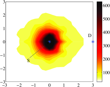
(a) Path-loss exponent $\alpha=2$.

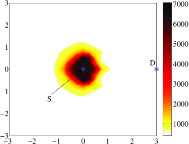
(b) Path-loss exponent $\alpha=4$.

Figure 1: Effect of eavesdropper location on link cost.

Effect of Optimal Secrecy Allocation on Path Cost. For a fixed path subject to an end-to-end secrecy requirement $\pi$, the optimal eavesdropping probability assigned to each link of the path is given by (42), which in turn determines the optimal jamming power allocated to each link of the path using (43). Specifically, this is how power allocation is performed in SASP in order to minimize power consumption. Alternatively, a simple heuristic is to divide $\pi$ equally across the links. That is, if the path contains $h$ links, then each link $\ell_{k}$ is allocated sufficient jamming power to satisfy the eavesdropping probability $\pi_{k}=\pi/h$. In Fig. 2, we have depicted energy savings that can be achieved “solely” by optimal secrecy allocation compared to equal allocation for a fixed path that is computed by SASP. Interestingly, as the number of eavesdroppers increases or the signal propagation becomes more restricted, optimal secrecy allocation becomes even more important, achieving energy savings of up to $72\%$ ($47\%$) for $\alpha=4$ ($\alpha=2$) in the simulated network.

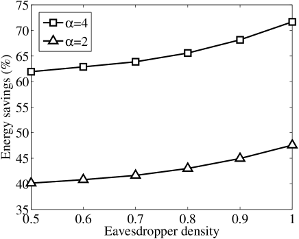
(a) Effect of eavesdropper density.

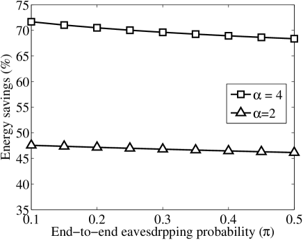
(b) Effect of eavesdropping prob.

Figure 2: Energy savings achieved by optimal secrecy allocation.

Non-uniform Eavesdropper Placement. To gain more insight about the behavior of different routing algorithms, in this experiment, rather than randomly distributing eavesdroppers in the network, we strategically place them close to the line that connects the source and destination. Ideally, SMER and $\epsilon$-SMER should avoid the shortest path that crosses the network diagonally. This is indeed the behavior observed in the simulations as depicted in Fig. 3 (‘ $\bigstar$ ’ denotes an eavesdropper). As expected, SASP blasts right through the eavesdroppers, while SMER, $0.1$-SMER and $1.0$-SMER route around them resulting in $88\%$, $86\%$ and $85\%$ energy savings, respectively.

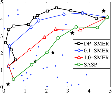
Figure 3: Snapshot of paths computed by different algorithms.

Uniform Eavesdropper Placement. In this experiment, eavesdroppers are placed in the network uniformly at random. As seen in Fig. 4, our algorithms consistently outperform SASP for a wide range of eavesdropper densities and eavesdropping probabilities. In particular, energy savings of up to $99\%$ and $98\%$ (for $\alpha=4$) can be achieved by SMER and $0.1$-SMER, respectively.

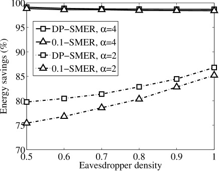
(a) Effect of eavesdropper density.

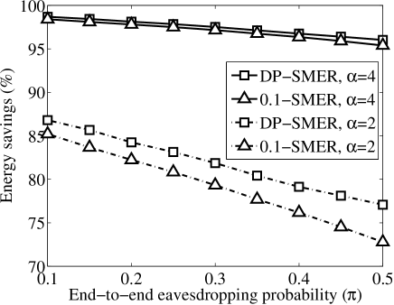
(b) Effect of eavesdropping prob.

Figure 4: Energy savings with uniform eavesdropper placement.

Effect of Network Size. Fig. 5 shows the energy savings achieved by different algorithms in networks with varying sizes. The “network dimension” refers to the length of one side of the square area that contains the network nodes. As observed from the figure, the energy saving is an increasing function of the network size. Interestingly, as the network size increases, the effect of the propagation environment diminishes in such a way that energy savings for $\alpha=2$ and $\alpha=4$ converge to the same numbers as opposed to the previous scenarios. As the network size increases so does the average length of the path (in terms of the number of hops) between the source and destination nodes. Those paths that are longer provide more opportunities for energy savings on each link of the path resulting in increased overall energy savings. This effect works in favor of $\alpha=2$ as well as $\alpha=4$. However, given the high values of energy savings for $\alpha=4$ (due to longer paths compared to $\alpha=2$), the effect of longer paths is more prominent for $\alpha=2$.

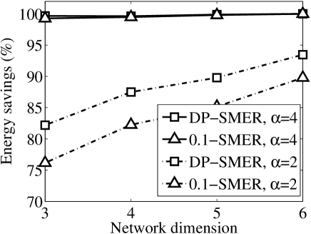
(a) Non-uniform eavesdrop. placement.

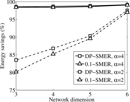
(b) Uniform eavesdrop. placement.

Figure 5: Effect of network size on energy savings.

Effect of Jamming Set. The cardinality of the jamming set affects the power allocation to jammers. In this experiment, we change the number of jammers that participate in secure transmissions on each link and compute the energy savings achieved by different algorithms. Figs. 6LABEL:sub@fig:jammers_diag and 6LABEL:sub@fig:jammers_uniform, respectively, show the energy savings achieved for non-unform and uniform placement of eavesdroppers. Interestingly, in these scenarios, a small number of jammers, namely $2$, is sufficient to obtain most of the benefits of cooperative jamming, which should greatly simplify any practical implementation.

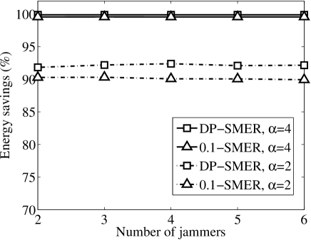
(a) Non-uniform eavesdrop. placement.

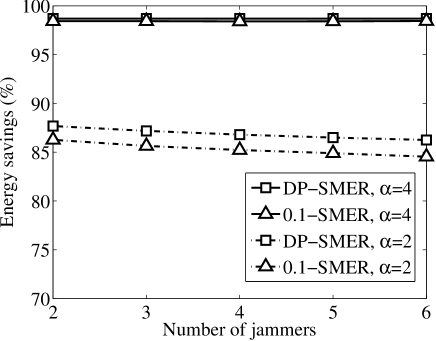
(b) Uniform eavesdrop. placement.

Figure 6: Effect of the jamming set on energy savings.

VII Related Work

A survey of prior work is presented in this section.

Secure Routing in Multi-hop Networks. While there are numerous works on secure routing in wireless networks (see, e.g., [35] and references therein), their focus is on preventing malicious attacks that disrupt the operation of the routing protocol using application level mechanisms such as authentication and cryptography. The focus of this paper, on the other hand, is on secure transmission of messages via the most cost-effective paths in the network, which is orthogonal to the secure routing problem considered in the existing literature.

Wireless Physical Layer Security. The idea behind physical layer security is to exploit the characteristics of the wireless channel such as fading to provide secure wireless communications. The foundations of information theoretic security, which is the theoretical basis for physical layer security, were laid by Wyner and others [4, 5, 6] based on Shannon’s notion of perfect secrecy [3]. In the classical wiretap model of Wyner, to achieve a strictly positive secrecy rate, the legitimate user should have some advantage over the eavesdropper in terms of SNR. Later, Maurer [7] proved that even when a legitimate user has a worse channel than an eavesdropper, it is possible to have secure communication. While some physical layer security techniques allow for opportunistic exploitation of the space/time/user diversity for secret communications [7, 8], others actively manipulate the wireless channel to block eavesdroppers by employing techniques such as multiple antennas [21] and jamming [10, 12]. While some of these techniques have been successfully implemented in practical systems [22], physical layer security is focused on very special network topologies, e.g., single-hop networks. In this work, we have developed algorithms to extend these techniques to multi-hop networks.

Scaling Laws in Large Secure Networks. Motivated by [36], recently, throughput scaling versus security tradeoffs have been investigated in the context of large wireless networks [17, 18, 19, 13]. Specifically, for cooperative jamming when the eavesdroppers are uniformly distributed, it was shown that if the number of eavesdroppers grows sub-linearly with respect to the number of legitimate nodes, a positive throughput for secure communication is achievable [13].

Security Based on Network Topology. When there is sufficient path diversity in a network, different messages can be routed over different parts of the network in the hope that an eavesdropper would be incapable of capturing all messages from across the network. To exploit network diversity for security, various techniques based on multi-path routing [37, 38] and network coding [39, 40] have been investigated. While such techniques are suitable for wired networks, their application in wireless networks is challenging due to lack of path diversity at the source or destination of a communication session. Moreover, there are considerable complications when splitting a flow among several paths, in particular, at the granularity of a single session. Moreover, network topology, in wireless networks, is a function of power allocation at the physical-layer and propagation environment, e.g., fading. Nevertheless, our approach is complimentary to these techniques, by providing a mechanism to find a minimum cost path that is information-theoretically secure, regardless of the network diversity.

VIII Conclusion

This paper studied the problem of secure minimum energy routing in wireless networks. It was shown that while the problem is NP-hard, it admits exact pseudo-polynomial and fully polynomial time $\epsilon$-approximation algorithmic solutions. Furthermore, using simulations, we showed that our algorithms significantly outperform security-agnostic algorithms based on minimum energy routing. Finally, we note that our work can be potentially extended to incorporate other secrecy models. Such extensions are left for future work.

References

- [1] D. Stinson, Cryptography: theory and practice. CRC press, 2006.
- [2] National Security Agency, “Defense in depth: A practical strategy for achieving information assurance in today’s highly networked environments.” [Online]. Available: http://www.nsa.gov/ia/_files/support/defenseindepth.pdf
- [3] C. Shannon, Communication theory of secrecy systems. AT&T, 1949.
- [4] A. Wyner, “The wire-tap channel,” Bell Sys. Tech. J., vol. 54, no. 8, 1975.
- [5] S. Leung-Yan-Cheong and M. Hellman, “The Gaussian wiretap channel,” IEEE Trans. Inf. Theory, vol. 24, no. 4, 1978.
- [6] I. Csiszár and J. Korner, “Broadcast channels with confidential messages,” IEEE Trans. Inf. Theory, vol. 24, no. 3, 1978.
- [7] U. M. Maurer, “Secret key agreement by public discussion from common information,” IEEE Trans. Inf. Theory, vol. 39, no. 3, 1993.
- [8] M. Bloch et al., “Wireless information-theoretic security,” IEEE Trans. Inf. Theory, vol. 54, no. 6, 2008.
- [9] S. Goel and R. Negi, “Guaranteeing secrecy using artificial noise,” IEEE Trans. Wireless Commun., vol. 7, no. 6, 2008.
- [10] E. Tekin and A. Yener, “The general Gaussian multiple-access and two-way wiretap channels: Achievable rates and cooperative jamming,” IEEE Trans. Inf. Theory, vol. 54, no. 6, 2008.
- [11] L. Dong, Z. Han, A. P. Petropulu, and H. V. Poor, “Improving wireless physical layer security via cooperating relays,” IEEE Trans. Signal Process., vol. 58, no. 3, 2010.
- [12] L. Lai and H. El Gamal, “The relay-eavesdropper channel: Cooperation for secrecy,” IEEE Trans. Inf. Theory, vol. 54, no. 9, 2008.
- [13] D. Goeckel et al., “Artificial noise generation from cooperative relays for everlasting secrecy in two-hop wireless networks,” IEEE J. Sel. Areas Commun., vol. 29, no. 10, 2011.
- [14] M. Haenggi, “The secrecy graph and some of its properties,” in IEEE ISIT, Jun. 2008.
- [15] P. Pinto, J. Barros, and M. Win, “Physical-layer security in stochastic wireless networks,” in IEEE ICCS, Nov. 2008.
- [16] ——, “Wireless physical-layer security: The case of colluding eavesdroppers,” in IEEE ISIT, Jun. 2009.
- [17] Y. Liang, H. Poor, and L. Ying, “Secrecy throughput of MANETs with malicious nodes,” in IEEE ISIT, Jun. 2009.
- [18] O. Koyluoglu, E. Koksal, and H. El Gamal, “On secrecy capacity scaling in wireless networks,” in IEEE ITA, Feb. 2010.
- [19] S. Vasudevan, D. Goeckel, and D. Towsley, “Security-capacity trade-off in large wireless networks using keyless secrecy,” in ACM Mobihoc, Sep. 2010.
- [20] J. Huang and A. L. Swindlehurst, “Robust secure transmission in MISO channels with imperfect ECSI,” in IEEE Globecom, 2011.
- [21] Z. Li, W. Trappe, and R. Yates, “Secret communication via multi-antenna transmission,” in CISS, Mar. 2007.
- [22] S. Gollakota et al., “They can hear your heartbeats: Non-invasive security for implantable medical devices,” in ACM Sigcomm, 2011.
- [23] S. Oh, T. Vu, M. Gruteser, and S. Banerjee, “Phantom: Physical layer cooperation for location privacy protection,” in IEEE Infocom, Orlando, USA, Mar. 2012.
- [24] D. Tse and P. Viswanath, Fundamentals of wireless communications. Cambridge, UK: Cambridge University Press, 2005.
- [25] A. Goldsmith, Wireless communications. Cambridge, 2005.
- [26] D. Seymour and J. Britton, Introduction to Tessellations. Palo Alto, USA: Dale Seymour Publications, 1990.
- [27] M. Dehghan, D. Goeckel, M. Ghaderi, and Z. Ding, “Energy efficiency of cooperative jamming strategies in secure wireless networks,” IEEE Transactions on Wireless Communications, vol. 54, no. 8, 2012.
- [28] R. Mudumbai, D. Brown, U. Madhow, and H. Poor, “Distributed transmit beamforming: challenges and recent progress,” IEEE Communications Magazine, vol. 47, no. 2, 2009.
- [29] M. Rahman, H. Baidoo-Williams, R. Mudumbai, and S. Dasgupta, “Fully wireless implementation of distributed beamforming on a software-defined radio platform,” in ADM/IEEE IPSN, 2012.
- [30] D. Brown, U. Madhow, P. Bidigare, and S. Dasgupta, “Receiver-coordinated distributed transmit nullforming with channel state uncertainty,” in Conference on Information Sciences and Systems (CISS), Mar. 2012.
- [31] G. L. Turin, “The characteristic function of hermitian quadratic forms in complex normal variables,” Biometrika, vol. 47, no. 1/2, 1960.
- [32] A. Shamir, “How to share a secret,” Commun. ACM, vol. 22, no. 11, 1979.
- [33] M. R. Garey and D. S. Johnson, Computers and interactability: A guide to the theory of NP-Completeness. New York, USA: W.H. Freeman and Company, 1979.
- [34] D. H. Lorenz and D. Raz, “A simple efficient approximation scheme for the restricted shortest path problem,” Operations Research Letters, vol. 28, 1999.
- [35] L. Abusalah et al., “A survey of secure mobile ad hoc routing protocols,” IEEE Commun. Surveys Tuts., vol. 10, no. 4, 2008.
- [36] P. Gupta and P. R. Kumar, “The capacity of wireless networks,” IEEE Trans. Inf. Theory, vol. 46, no. 2, 2000.
- [37] W. Lou, W. Liu, Y. Zhang, and Y. Fang, “SPREAD: Improving network security by multipath routing in mobile ad hoc networks,” ACM Wireless Networks, vol. 15, no. 3, 2009.
- [38] T. Shu, M. Krunz, , and S. Liu, “Secure data collection in wireless sensor networks using randomized dispersive routes,” IEEE Trans. Mobile Comput., vol. 9, no. 7, 2010.
- [39] N. Cai and R. W. Yeung, “Secure network coding,” in IEEE ISIT, Jun. 2002.
- [40] K. Jain, “Security based on network topology against the wiretapping attack,” IEEE Wireless Commun. Mag., vol. 11, no. 1, 2004.