Modeling Nucleon Generalized Parton Distributions

Abstract

We discuss building models for nucleon generalized parton distributions (GPDs) $H$ and $E$ that are based on the formalism of double distributions (DDs). We found that the usual “DD+D-term” construction should be amended by an extra term, $\xi E_{+}^{1}(x,\xi)$ built from the $\alpha/\beta$ moment of the DD $e(\beta,\alpha)$ that generates GPD $E(x,\xi)$. Unlike the $D$-term, this function has support in the whole $-1\leq x\leq 1$ region, and in general does not vanish at the border points $|x|=\xi$.

I Introduction

The studies of Generalized Parton Distributions (GPDs) Mueller et al. (1994); Ji (1997); Radyushkin (1996); Collins et al. (1997) require building theoretical models for GPDs which satisfy several nontrivial requirements such as polynomiality Ji (1998), positivity Martin and Ryskin (1998); Pire et al. (1999); Radyushkin (1999), hermiticity Mueller et al. (1994), time reversal invariance Ji (1998), etc. The constraints follow from the most general principles of quantum field theory. Polynomiality (that may be traced back to Lorentz invariance) imposes the restriction that $x^{n}$ moment of a GPD $H(x,\xi;t)$ must be a polynomial in $\xi$ of the order not higher than $n+1$. This property is automatically obeyed by GPDs constructed from Double Distributions (DDs) Mueller et al. (1994); Radyushkin (1996, 1996, 1999). (Another way to impose the polynomiality condition onto model GPDs is “dual parameterization” Polyakov and Shuvaev (2002); Polyakov (2007, 2008); Semenov-Tian-Shansky (2008); Polyakov and Semenov-Tian-Shansky (2009)). Thus, within the DD approach, the problem of constructing a model for a GPD converts into a problem of building a model for the relevant DD.

Double distributions $F(\beta,\alpha;t)$ behave like usual parton distribution functions (PDFs) with respect to its variable $\beta$, as a meson distribution amplitude (DA) with respect to $\alpha$, and as a form factor with respect to the invariant momentum transfer $t$. The factorized DD ansatz (FDDA) Radyushkin (1999, 1999) proposes to build a model DD $F(\beta,\alpha)$ (in the simplified formal $t=0$ limit) as a product of the usual parton density $f(\beta)$ and a profile function $h(\beta,\alpha)$ that has an $\alpha$-shape of a meson DA. However, it was noticed Polyakov and Weiss (1999) that in the case of isosinglet pion GPDs, FDDA does not produce the highest, $(n+1)^{\rm st}$ power of $\xi$ in the $x^{n}$ moment of $H(x,\xi)$. To cure this problem, a “two-DD” parameterization for pion GPDs was proposed Polyakov and Weiss (1999), with the second DD $G(\beta,\alpha)$ capable of generating, among others, the required $\xi^{n+1}$ power. It was also proposed Polyakov and Weiss (1999) to use a “DD plus D” parameterization in which the second DD $G(\beta,\alpha)$ is reduced to a function $D(\alpha)$ of one variable, the $D$-term , that is solely responsible for the $\xi^{n+1}$ contribution. As emphasized in Ref. Polyakov and Weiss (1999), one should also add $D$-term in case of nucleon distributions. The importance of the $D$-term and its physical interpretation were studied in further works (see Ref. Goeke et al. (2001) and references therein).

In the pion case, it was shown Teryaev (2001) that one can reshuffle terms between $F$ and $G$ functions of the $F+G$ decomposition without changing the sum (“gauge invariance”). Furthermore, it was found in Ref. Belitsky et al. (2002), that one can write a parameterization that incorporates just one function $f(\beta,\alpha)$, but still produces all the required powers up to $\xi^{n+1}$. A model for the pion GPD based on this representation was built in our paper Radyushkin (2011). An important ingredient of our construction was separation of DD $f(\beta,\alpha)$ in its “plus” part $[f(\beta,\alpha)]_{+}$ that gives zero after integration over $\beta$, and $D$-term part $\delta(\beta)D(\alpha)/\alpha$. For DDs singular in small-$\beta$ region, such a separation serves also as a renormalization prescription substituting a formally divergent integral over $\beta$ by “observable” $D$-term.

In the present paper, we apply the technique of Ref. Radyushkin (2011) (see also Radyushkin (2012)) for building models of nucleon GPDs $H(x,\xi)$ and $E(x,\xi)$. The paper is organized as follows. To make it self-contained, we start, in Sect. II, with a short review of the basic facts about DDs, GPDs and $D$-term, using a toy model with scalar quarks, that allows to illustrate essential features of GPD theory avoiding complications related to spin. In Sect. III, we describe the theory of pion GPD $H(x,\xi)$, presenting the results of Ref. Radyushkin (2011) in a form suitable for generalization onto the nucleon case. In Sect. IV, we recall the basic ideas of the factorized DD Ansatz of Refs. Radyushkin (1999, 1999). In Sect. V, we use the formalism described in previous sections for building DD models for nucleon GPDs $H(x,\xi)$ and $E(x,\xi)$.

An essential point is that two functions $A$ and $B$ associated with two basic Dirac structures present in the twist decomposition of the nucleon matrix element do not coincide with $H$ and $E$. In fact, $A=H+E$ and $B=-E$. What is most important, $A$ and $B$ have different types of DD representation: $A$ is given by the simplest (scalar-type) DD representation, while $B$ is given by a more complicated representation coinciding with the one-DD parametrization of the pion case. Thus, building a model for $H$ one should deal with a sum $A+B$, the terms of which have different-type DD representations. The result of this mismatch is a term, which we call $\xi E_{+}^{1}(x,\xi)$ that is given by the “plus” part of the $\alpha/\beta$ moment of DD $e(\beta,\alpha)$ used in parametrization for $E(x,\xi)$ GPD. The term $\xi E_{+}^{1}(x,\xi)$ should be included in the model for GPD $H(x,\xi)$. However, unlike the $D$-term contribution, the function $\xi E_{+}^{1}(x,\xi)$ in general does not vanish both at the border points $|x|=\xi$ and also outside the central region $|x|\leq\xi$.

In final section, we summarize the results of the paper.

II Basics of theory for DDs and GPDs

II.1 Matrix elements and DDs

Parton distributions provide a convenient way to parametrize matrix elements of local operators that accumulate information about hadronic structure. Various types of distributions differ by the nature of the matrix elements involved. In particular, to define GPDs, one starts with non-forward matrix elements $\langle P+r/2|\ldots|P-r/2\rangle$, with $P$ being the average of the initial and final hadron momenta, and $r$ being their difference. In scalar case (which illustrates many essential features without irrelevant complications) we have

$$\langle P+r/2|\psi(0)\{\stackrel{{\scriptstyle\leftrightarrow}}{{\partial}}_{\mu_{1}}\ldots\stackrel{{\scriptstyle\leftrightarrow}}{{\partial}}_{\mu_{n}}\}\psi(0)|P-r/2\rangle$$

$$=\sum_{l=0}^{n-1}A_{nl}\{P_{\mu_{1}}\ldots P_{\mu_{n-l}}r_{\mu_{n-l+1}}\ldots r_{\mu_{n}}\}$$

$$+A_{nn}\{r_{\mu_{1}}\ldots r_{\mu_{n}}\}\ .$$ (1)

The notation $\{\ldots\}$ indicates the symmetric-traceless part of the enclosed tensor. Since two vectors are involved, we have $n+1$ distinct tensor structures differing in the number $l$ of $r$ factors involved. In the forward $r=0$ limit, only the $A_{n_{0}}$ coefficients are visible. Another extreme case is $l=n$, corresponding to the tensor $\{r_{\mu_{1}}\ldots r_{\mu_{n}}\}$ built solely from the $r$ momentum.

The forward $r=0$ limit corresponds to matrix elements defining usual parton distributions $f(x)$ as a function whose moments produce $A_{n0}$:

$$\int_{-1}^{1}f(x)x^{n}\,dx=A_{n_{0}}\ .$$ (2)

The parton interpretation of $f(x)$ is that it describes a parton with momentum $xP$. This definition of $f(x)$ may be rewritten in terms of matrix elements of operators on the light cone:

$$\langle P|\psi(-z/2)\psi(z/2)|P\rangle$$

$$=\int_{-1}^{1}f(x)\,e^{-ix(Pz)}\,dx\,+{\cal O}(z^{2})\ .$$ (3)

In a general non-forward case, the parton carries the fractions of both $P$ and $r$ momenta. Note, that in the momentum representation, the derivative $\stackrel{{\scriptstyle\leftrightarrow}}{{\partial}}_{\mu}\$ converts into the average $\bar{k}_{\mu}=(k_{\mu}+k^{\prime}_{\mu})/2$ of the initial $k$ and final $k^{\prime}$ quark momenta. After integration over $k$, $(\bar{k})^{n}$ should produce the $P$ and $r$ factors in the r.h.s. of Eq. (1). In this sense, one may treat $(\bar{k})^{n}$ as $(\beta P+\alpha r/2)^{n}$ and define the double distribution (DD) Mueller et al. (1994); Radyushkin (1996, 1996, 1999)

$$\frac{n!}{(n-l)!\,l!\,2^{l}}\int_{\Omega}F(\beta,\alpha)\beta^{n-l}\alpha^{l}\,d\beta\,d\alpha=A_{nl}$$ (4)

as a function whose $\beta^{n-l}\alpha^{l}$ moments are proportional to the coefficients $A_{nl}$. It can be shown Mueller et al. (1994); Radyushkin (1996, 1999) that the support region $\Omega$ is given by the rhombus $|\alpha|+|\beta|\leq 1$. These definitions result in the “DD parameterization”

$$\langle P-r/2|\psi(-z/2)\psi(z/2)|P+r/2\rangle$$

$$=\int_{\Omega}F(\beta,\alpha)\,e^{-i\beta(Pz)-i\alpha(rz)/2}\,d\beta\,d\alpha+{\cal O}(z^{2})\ .$$ (5)

of the matrix element.

II.2 Introducing GPDs and $D$-term

Another parametrization of the non-forward matrix element is in terms of generalized parton distributions. In scalar case GPDs are defined by

$$\langle P-r/2|\psi(-z/2)\psi(z/2)|P+r/2\rangle$$

$$=\int_{-1}^{1}\,e^{-ix(Pz)}H(x,\xi)\,dx+{\cal O}(z^{2})\ ,$$ (6)

and relation between GPD and DD functions is given by

$$H(x,\xi)=\int_{\Omega}F(\beta,\alpha)\,\delta(x-\beta-\xi\alpha)\,d\beta\,d\alpha\ .$$ (7)

The skewness parameter $\xi$ in this definition corresponds to the ratio $(rz)/2(Pz)$.

In the forward limit $\xi=0$, GPD $H(x,\xi)$ converts into the usual parton distribution $f(x)$. Using DDs, we may write

$$f(x) =\int_{-1+|x|}^{1-|x|}F(x,\alpha)\,d\alpha\ .$$ (8)

Thus, the forward distributions $f(x)$ are obtained by integrating DDs over vertical lines $\beta=x$ in the $(\beta,\alpha)$ plane. As discussed above, $f(x)$ is defined through the coefficients $A_{n0}$ corresponding to tensors without $r$ factors. Similarly, one can treat the $A_{nn}$ coefficients, corresponding to tensors without $P$ factors, as the moments of another function $D(\alpha)$

$$\int_{-1}^{1}D(\alpha)\,(\alpha/2)^{n}\,d\alpha=A_{nn}\ ,$$ (9)

the $D$-term Polyakov and Weiss (1999). From the definition of DD (4), it follows that

$$D(\alpha)=\int_{-1+|\alpha|}^{1-|\alpha|}F(\beta,\alpha)\,d\beta\ ,$$ (10)

i.e., $D$-term $D(\alpha)$ is obtained from DD $F(\beta,\alpha)$ by integration over horizontal lines in the $\{\beta,\alpha\}$ plane. In this sense, one can think of “vertical” projection of DD that produces the forward distribution $f(\beta)$, and “horizontal” projection that produces $D$-term $D(\alpha)$.

Taking the $x^{n}$ moment of GPD $H(x,\xi)$

$$\int_{-1}^{1}\,H(x,\xi)\,x^{n}\,dx=\sum_{l=0}^{n}A_{nl}(2\xi)^{l}\ ,$$ (11)

we see that the coefficients $A_{nn}$ are responsible for the highest power of skewness $\xi$ in this expansion.

II.3 DD plus D parametrization

Parameterizing the matrix element (1), one may wish to separate the $A_{nn}$ terms that are accompanied by tensors built from the momentum transfer vector $r$ only, and, thus, are invisible in the forward $r=0$ limit, i.e., to separate the $D$-term contribution. This can be made by simply using

$$e^{-i\beta(Pz)}=[e^{-i\beta(Pz)}-1]+1$$ (12)

which converts the DD-parameterization into a “DD₊ plus D” parameterization

$$\langle P-r/2|\psi(-z/2)\psi(z/2)|P+r/2\rangle$$

$$=\int_{\Omega}[F(\beta,\alpha)]_{+}\,e^{-i\beta(Pz)-i\alpha(rz)/2}\,d\beta\,d\alpha$$

$$+\int_{-1}^{1}D(\alpha)\,e^{-i\alpha(rz)/2}\,d\alpha+{\cal O}(z^{2})\ ,$$ (13)

where

$$[F(\beta,\alpha)]_{+}=F(\beta,\alpha)-\delta(\beta)\int_{-1+|\alpha|}^{1-|\alpha|}F(\gamma,\alpha)\,d\gamma$$ (14)

is the DD with subtracted $D$-term given by Eq.(10). Then

$$F(\beta,\alpha)=[F(\beta,\alpha)]_{+}+\delta(\beta)D(\alpha)$$ (15)

and

$$H(x,\xi)=H_{+}(x,\xi)+\frac{D(x/\xi)}{|\xi|}\ ,$$ (16)

where

$$H_{+}(x,\xi)= \int_{\Omega}[F(\beta,\alpha)]_{+}\,\delta(x-\beta-\xi\alpha)\,d\beta\,d\alpha$$

$$=\int_{\Omega}F(\beta,\alpha)\,\Big{[}\delta(x-\beta-\xi\alpha)$$

$$\hskip 56.9055pt-\delta(x-\xi\alpha)\Big{]}\,d\beta\,d\alpha$$ (17)

is the “plus” part of GPD $H(x,\xi)$.

A straightforward observation is that the $x^{n}$ moment of $H_{+}(x,\xi)$ does not contain the highest, namely the $n^{\rm th}$ power of $\xi$, since the relevant integral

$$\int_{\Omega}\alpha^{n}\,\left[F(\beta,\alpha)\right]_{+}\,\,d\beta\,d\alpha$$ (18)

vanishes because the integrand is a “plus” distribution with respect to $\beta$.

For $n=0$, the highest power is $\xi^{0}$, and since the $n=0$ moment of $H_{+}(x,\xi)$ should not contain this highest power, it contains no powers of $\xi$ at all, i.e. it vanishes:

$$\int_{-1}^{1}\,H_{+}(x,\xi)\,dx=\int_{\Omega}\left[F(\beta,\alpha)\right]_{+}\,\,d\beta\,d\alpha=0\ .$$ (19)

Thus, $H_{+}(x,\xi)$ has the same property with respect to integration over $x$ as a “plus” distribution

$$[h(x)]_{+}=h(x)-\delta(x)\int_{-1}^{1}h(z)dz\ .$$ (20)

However, $H_{+}(x,\xi)$ may be a pretty smooth function, without any $\delta(x)$ terms. It should just possess regions of positive and negative values of $H_{+}(x,\xi)$ averaging to zero after $x$-integration.

II.4 $D$-term as a separate entity

In the simple model with scalar quarks, one may just use the original DD $F(\beta,\alpha)$ without splitting it into the “plus” part and the $D$-term. One may imagine that the DD $F(\beta,\alpha)$ is some smooth function on the rhombus, with nothing spectacular happening on the $\beta=0$ line. In such a case, one may, of course, write $F(\beta,\alpha)=[F(\beta,\alpha)]_{+}+\delta(\beta)D(\alpha)$, with the $D$-term accompanied by the $\delta(\beta)$ function, but this term is precisely canceled by the $\sim\delta(\beta)$ term contained in $[F(\beta,\alpha)]_{+}$.

However, if the theory allows purely $t$-channel exchanges, then the relevant diagrams generate $\sim\delta(\beta)$ terms not necessarily connected to other contributions. E.g., our scalar quarks may have a quartic interaction, and the $t$-channel loop would generate a $\delta(\beta)\varphi(\alpha)$ type contribution into $F(\beta,\alpha)$.

Furthermore, $D$ term is formally given by the integral of $F(\beta,\alpha)$. An implicit assumption is that this integral converges, which is the case if $F(\beta,\alpha)$ is not too singular. Note, however, that the integral of $F(\beta,\alpha)$ over $\alpha$ gives $f(\beta)$, a usual parton distribution which are known to have a singular $\sim\beta^{-a}$ behavior for small $\beta$. This means that the $\beta$-profile of DD $F(\beta,\alpha)$ should be similar to that of $f(\beta)$, and also be singular in the $\beta\to 0$ region, $F(\beta,\alpha)\sim\beta^{-a}$. The integral over $\beta$ converges if $a<1$. However, as we will see in Sec. III B, one may need the integrals involving $F(\beta,\alpha)/\beta$ which diverge for any positive $a$. The integral for $[F(\beta,\alpha)]_{+}$ still converges for $a<1$, and the role of the $D$ term in this case is to substitute the divergent integral

$$\int_{-1+|\alpha|}^{1-|\alpha|}F(\beta,\alpha)\,d\beta$$ (21)

by a finite function $D(\alpha)$ whose $\alpha^{n}$ moments then give finite coefficients $A_{nn}$. In this case, the “DD₊ plus D” separation serves as a renormalization prescription defining the moments of DD.

An attempt to consistently “implant” the Regge behavior into a quantum field theory construction was made in Ref. Szczepaniak et al. (2009), where a dispersion relation was used for an amplitude that has $s^{a}$ Regge behavior at large energies. For any positive $a$, such a relation requires a subtraction, which (as shown in Refs.Szczepaniak et al. (2009); Radyushkin (2011)) results in a $\delta(\beta)\varphi(\alpha)$ term contributing to $D(\alpha)$.

III Pion DDs and GPDs

III.1 Two-DD representation

In fact, $D$-term was introduced first Polyakov and Weiss (1999) in the context of pion GPDs, with pion made of spinor quarks. In that case, it is more difficult to avoid an explicit introduction of the $D$-term as an extra function. The basic reason is that the matrix element of the bilocal operator in pion case has two parts

$$\langle P-r/2|\bar{\psi}(-z/2)\gamma_{\mu}\psi(z/2)|P+r/2\rangle|_{\rm twist-2}$$

$$=2P_{\mu}f\bigl{(}(Pz),(rz),z^{2}\bigr{)}+r_{\mu}g\bigl{(}(Pz),(rz),z^{2}\bigr{)}\ .$$ (22)

This suggests a parametrization with two DDs corresponding to $f$ and $g$ functions Polyakov and Weiss (1999). For the matrix element (22) multiplied by $z^{\mu}$ (the object one obtains doing the leading-twist factorization for the Compton amplitude Balitsky and Braun (1989) ) this gives

$$z^{\mu}\langle P-r/2|\bar{\psi}(-z/2)\gamma_{\mu}\psi(z/2)|P+r/2\rangle$$

$$=\int_{\Omega}e^{-i\beta(Pz)-i\alpha(rz)/2}\,\biggl{[}2(Pz)F(\beta,\alpha)$$

$$+(rz)G(\beta,\alpha)\biggr{]}\,d\beta\,d\alpha\ +{\cal O}(z^{2}).$$ (23)

Then GPDs are given by a DD representation

$$H(x,\xi)=\int_{\Omega}\bigl{[}F(\beta,\alpha)+\xi G(\beta,\alpha)\bigr{]}\,\delta(x-\beta-\xi\alpha)\,d\beta\,d\alpha\ ,$$ (24)

that involves two DDs: $F(\beta,\alpha)$ and $G(\beta,\alpha)$. The highest power $\xi^{n+1}$ for the $x^{n}$ moment of $H(x,\xi)$ is given now by the $G$ term, which one can separate

$$G(\beta,\alpha)=[G(\beta,\alpha)]_{+}+\delta(\beta)D(\alpha)$$ (25)

into a “plus” part and $D$-term

$$D(\alpha)=\int_{-1+|\alpha|}^{1-|\alpha|}G(\beta,\alpha)\,d\beta\ .$$ (26)

As a result,

$$H(x,\xi)=F(x,\xi)+\xi G_{+}(x,\xi)+{\rm sgn}(\xi){D(x/\xi)}\ ,$$ (27)

where

$$F(x,\xi)=\int_{\Omega}F(\beta,\alpha)\,\delta(x-\beta-\xi\alpha)\,d\beta\,d\alpha$$ (28)

and

$$G_{+}(x,\xi)=\int_{\Omega}G(\beta,\alpha)\,\Big{[} \delta(x-\beta-\xi\alpha)$$

$$-\delta(x-\xi\alpha)\Big{]}\,d\beta\,d\alpha\ .$$ (29)

The forward distribution $f(x)$ in two-DD formulation is obtained from the DD $F$ only:

$$f(\beta) =\int_{-1+|\beta|}^{1-|\beta|}F(\beta,\alpha)\,d\alpha\ .$$ (30)

Thus, $D$-term and $f(x)$ are obtained from different functions, so the $D$-term is indeed looking like an independent entity.

III.2 One-DD representation

Note that the Dirac index $\mu$ is symmetrized in the local twist-two operators $\bar{\psi}\{\gamma_{\mu}\stackrel{{\scriptstyle\leftrightarrow}}{{\partial}}_{\mu_{1}}\ldots\stackrel{{\scriptstyle\leftrightarrow}}{{\partial}}_{\mu_{n}}\}\psi$ with the $\mu_{i}$ indices related to the derivatives. Thus, one may expect that it also produces the factor $\beta P_{\mu}+\alpha r_{\mu}/2$. In Ref. Belitsky et al. (2001), it was shown that this is really the case. In other words, not only the exponential produces the $z$-dependence in the combination $\beta(Pz)+\alpha(rz)/2$, but also the pre-exponential terms come in the $\beta(Pz)+\alpha(rz)/2$ combination. The result is a representation in which

$$2(Pz)F(\beta,\alpha)+(rz)G(\beta,\alpha)$$

$$=[2\beta(Pz)+\alpha(rz)]f(\beta,\alpha)\ ,$$ (31)

that corresponds to

$$F(\beta,\alpha)=\beta f(\beta,\alpha)$$

and

$$G(\beta,\alpha)=\alpha f(\beta,\alpha)\ .$$

Thus, one deals formally with just one DD $f(\beta,\alpha)$. The two-DD representation for GPDs (24) converts into

$$H(x,\xi) =\int_{\Omega}(\beta+\xi\alpha)f(\beta,\alpha)\,\delta(x-\beta-\xi\alpha)\,d\beta\,d\alpha$$

$$=x\int_{\Omega}f(\beta,\alpha)\,\delta(x-\beta-\xi\alpha)\,d\beta\,d\alpha$$ (32)

in the “one-DD” formulation.

The $D$-term in the one-DD case is given by

$$D(\alpha)=\alpha\int_{-1+|\alpha|}^{1-|\alpha|}f(\beta,\alpha)\,d\beta\ ,$$ (33)

and one may write $f(\beta,\alpha)$ as a sum

$$f(\beta,\alpha)=[f(\beta,\alpha)]_{+}+\delta(\beta)\frac{D(\alpha)}{\alpha}$$ (34)

of its “plus” part

$$[f(\beta,\alpha)]_{+}=f(\beta,\alpha)-\delta(\beta)\int_{-1+|\alpha|}^{1-|\alpha|}f(\gamma,\alpha)\,d\gamma$$ (35)

and $D$-term part $\delta(\beta){D(\alpha)}/{\alpha}$.

For the GPD $H(x,\xi)$, the “DD₊+ D” separation corresponds to the representation

$$H(x,\xi)\equiv H_{+}(x,\xi)+{\rm sgn}(\xi)D(x/\xi)\ ,$$ (36)

where

$$\frac{H_{+}(x,\xi)}{x}\equiv\int_{\Omega}f(\beta,\alpha)\,\Big{[} \delta(x-\beta-\xi\alpha)$$

$$-\delta(x-\xi\alpha)\Big{]}\,d\beta\,d\alpha\ .$$ (37)

Using $f(\beta,\alpha)=F(\beta,\alpha)/\beta$ we may rewrite

$$H(x,\xi)=\int_{\Omega}(\beta+\xi\alpha)f(\beta,\alpha)\,\delta(x-\beta-\xi\alpha)\,d\beta\,d\alpha$$

$$=\int_{\Omega}F(\beta,\alpha)\,\delta(x-\beta-\xi\alpha)\,d\beta\,d\alpha$$

$$+\xi\int_{\Omega}\frac{\alpha F(\beta,\alpha)}{\beta}\Big{[}\delta(x-\beta-\xi\alpha)-\delta(x-\xi\alpha)\Big{]}\,d\beta\,d\alpha$$

$$+{\rm sgn}(\xi)D(x/\xi)$$

$$\equiv F_{DD}(x,\xi)+\xi F^{1}_{+}(x,\xi)+{\rm sgn}(\xi)D(x/\xi)\ ,$$ (38)

where

$$F_{DD}(x,\xi)=\int_{\Omega}F(\beta,\alpha)\,\delta(x-\beta-\xi\alpha)\,d\beta\,d\alpha$$ (39)

is GPD constructed from DD $F(\beta,\alpha)$ by the same formula as in scalar case. Another term

$${F^{1}_{+}(x,\xi)}\equiv\int_{\Omega}\left(\frac{\alpha}{\beta}\,F(\beta,\alpha)\right)_{+}\,\delta(x-\beta-\xi\alpha)\,d\beta\,d\alpha$$ (40)

is a GPD built from the “plus” part of the DD $\alpha F(\beta,\alpha)/\beta$. The latter, of course, may be written as $G(\beta,\alpha)$, but in the spirit of the one-DD formulation, one may wish to express the results in terms of just one function $F(\beta,\alpha)$.

IV Factorized DD Ansatz

In the forward limit $\xi=0$, GPD $H(x,\xi)$ converts into the usual parton distribution $f(x)$. In the one- DD formulation, we may write

$$f(x) =x\int_{-1+|x|}^{1-|x|}f(x,\alpha)\,d\alpha\ .$$ (41)

Thus, the forward distributions $f(x)$ are obtained by integrating over vertical lines $\beta=x$ in the $(\beta,\alpha)$ plane. For nonzero $\xi$, GPDs are obtained from DDs through integrating them along the lines $\beta=x-\xi\alpha$ having $1/\xi$ slope. The reduction formula (41) suggests the factorized DD Ansatz

$$f(\beta,\alpha)=h(\beta,\alpha)\,{f(\beta)}/{\beta}\ ,$$ (42)

where $f(\beta)$ is the forward distribution, while $h(\beta,\alpha)$ determines DD profile in the $\alpha$ direction and satisfies the normalization condition

$$\int_{-1+|\beta|}^{1-|\beta|}h(\beta,\alpha)\,d\alpha=1\ .$$ (43)

The profile function should be symmetric with respect to $\alpha\to-\alpha$ because DDs $f(\beta,\alpha)$ are even in $\alpha$ Mankiewicz et al. (1998); Radyushkin (1999). For a fixed $\beta$, the function $h(\beta,\alpha)$ describes how the longitudinal momentum transfer $r^{+}$ is shared between the two partons. Hence, it is natural to expect that the shape of $h(\beta,\alpha)$ should look like a symmetric meson distribution amplitude (DA) $\varphi(\alpha)$. Since DDs have the support restricted by $|\alpha|\leq 1-|\beta|$, to get a more complete analogy with DAs, it makes sense to rescale $\alpha$ as $\alpha=(1-|\beta|)\gamma$ introducing the variable $\gamma$ with $\beta$-independent limits: $-1\leq\gamma\leq 1$. The simplest model is to assume that the $\gamma$–profile is a universal function $g(\gamma)$ for all $\beta$. Possible simple choices for $g(\gamma)$ may be $\delta(\gamma)$ (no spread in $\gamma$-direction), $\frac{3}{4}(1-\gamma^{2})$ (characteristic shape for asymptotic limit of nonsinglet quark distribution amplitudes), $\frac{15}{16}(1-\gamma^{2})^{2}$ (asymptotic shape of gluon distribution amplitudes), etc. In the variables $\beta,\alpha$, these models can be treated as specific cases of the general profile function

$$h^{(N)}(\beta,\alpha)=\frac{\Gamma(2N+2)}{2^{2N+1}\Gamma^{2}(N+1)}\frac{[(1-|\beta|)^{2}-\alpha^{2}]^{N}}{(1-|\beta|)^{2N+1}}\,,$$ (44)

whose width is governed by the parameter $N$.

To give a graphical example, we show in Fig.1 the simplest GPD $F_{DD}(x,\xi)$ (39) built from the model

$$F(\beta,\alpha)={f(\beta)}h^{(1)}(\beta,\alpha)$$ (45)

with forward distribution

$$f^{\rm mod}(x)=(1-x)^{3}/\sqrt{x}$$ (46)

and $N=1$ profile function (analytic results for $f^{\rm mod}(x)=(1-x)^{3}x^{-a}$ and $N=1$ profile may be found in Refs. Musatov and Radyushkin (2000); Radyushkin (2000); Belitsky and Radyushkin (2005)).

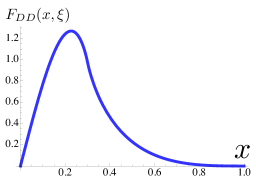
Figure 1: GPD $F_{DD}(x,\xi)$ for $\xi=0.3$.

The model forward function was chosen in the form reproducing the $x\to 1$ behavior of the nucleon parton distributions and the $\sim x^{-0.5}$ Regge behavior of valence part of quark distributions for small $x$, which was taken for simplicity, though the GPD shown corresponds to the $C$-even component (the full function is antisymmetric in $x$, and only the $x\geq 0$ part is shown).

V Nucleon GPDs

V.1 Definitions of DDs and GPDs

In the nucleon case, for unpolarized target, one can parametrize

$$\langle p^{\prime}|\bar{\psi}(-z/2)\not{z}\,\psi(z/2)|p\rangle|_{\rm twist-2}$$ (47)

$$=\int_{\Omega}e^{-i\beta(Pz)-i\alpha(rz)/2}\,\Big{[}\bar{u}(p^{\prime})\not{z}\,u(p)\,a(\beta,\alpha)$$

$$+\frac{\bar{u}(p^{\prime})u(p)}{2M_{N}}\,\big{[}2\beta(Pz)+\alpha(rz)\big{]}b(\beta,\alpha)\Big{]}\,d\beta\,d\alpha\ +{\cal O}(z^{2})\ .$$

Here, the functions $a,b$ are DDs corresponding to the combinations $A=H+E$ and $B=-E$ of usual GPDs $H$ and $E$ (see Ref. Belitsky and Radyushkin (2005)). These GPDs may be expressed in terms of relevant DDs as

$${A(x,\xi)}=\int_{\Omega}a(\beta,\alpha)\,\delta(x-\beta-\xi\alpha)\,d\beta\,d\alpha$$ (48)

and

$${B(x,\xi)}={x}\int_{\Omega}b(\beta,\alpha)\,\delta(x-\beta-\xi\alpha)\,d\beta\,d\alpha\ .$$ (49)

Notice that we have two different types of relations between GPDs and DDs: $A(x,\xi)$ is obtained from its DD $a(\beta,\alpha)$ just like in the simplest scalar case, while $B(x,\xi)$ is calculated from $b(\beta,\alpha)$ using the formula with the one-DD representation structure. The difference, of course, is due to the factor $[2\beta(Pz)+\alpha(rz)]$ in the $b$-part.

In the forward limit, we have

$$A(x,0)=H(x,0)+E(x,0)=f(x)+e(x)$$ (50)

and

$$B(x,0)=-E(x,0)=-e(x)\ .$$ (51)

These reduction formulas suggest the model representation

$$a(\beta,\alpha)=f(\beta,\alpha)+e(\beta,\alpha)$$ (52)

and

$$b(\beta,\alpha)=-\frac{e(\beta,\alpha)}{\beta}\ .$$ (53)

Because of possible singularity of $e(\beta,\alpha)/\beta$ at $\beta=0$, we write it in the “DD${}_{+}+D$” representation:

$$b(\beta,\alpha)=-\left(\frac{e(\beta,\alpha)}{\beta}\right)_{+}+\delta(\beta)\frac{D(\alpha)}{\alpha}\ ,$$ (54)

where $D(\alpha)$ is the $D$-term.

V.2 General results for GPDs

As a result, we have

$${H(x,\xi)}={A(x,\xi)}+{B(x,\xi)}$$ (55)

$$=\int_{\Omega}[f(\beta,\alpha)+e(\beta,\alpha)]\,\delta(x-\beta-\xi\alpha)\,d\beta\,d\alpha$$

$$-x\int_{\Omega}\left[\left(\frac{e(\beta,\alpha)}{\beta}\right)_{+}-\delta(\beta)\frac{D(\alpha)}{\alpha}\right]\,\delta(x-\beta-\xi\alpha)\,d\beta\,d\alpha$$

$$=F_{DD}(x,\xi)+E_{DD}(x,\xi)-E_{+}(x,\xi)+{\rm sgn}(\xi)\,D(x/\xi)\ ,$$

where

$$F_{DD}(x,\xi)=\int_{\Omega}f(\beta,\alpha)\,\delta(x-\beta-\xi\alpha)\,d\beta\,d\alpha$$ (56)

and

$$E_{DD}(x,\xi)=\int_{\Omega}e(\beta,\alpha)\,\delta(x-\beta-\xi\alpha)\,d\beta\,d\alpha$$ (57)

are build from DDs by simplest formulas not involving a division by $\beta$ factors, while

$$\frac{E_{+}(x,\xi)}{x}= \int_{\Omega}\frac{e(\beta,\alpha)}{\beta}\Big{[}\,\delta(x-\beta-\xi\alpha)-\delta(x-\xi\alpha)\Big{]}\,d\beta\,d\alpha$$

$$=\int_{\Omega}\left(\frac{e(\beta,\alpha)}{\beta}\right)_{+}\delta(x-\beta-\xi\alpha)\,d\beta\,d\alpha$$ (58)

has the structure of a one-DD representation. Since $E_{+}(x,\xi)/x$ is built from the “plus” part of a DD it should satisfy

$$\int_{-1}^{1}\,E_{+}(x,\xi)\,dx=\int_{\Omega}\left[\frac{e(\beta,\alpha)}{\beta}\right]_{+}\,\,d\beta\,d\alpha=0\ .$$ (59)

Figure 2: GPD $E_{+}(x,\xi)$ for $\xi=0.3$.

Being (for $C$-even combination) an even function of $x$, the function $E_{+}(x,\xi)/x$ obeys

$$\int_{0}^{1}\frac{E_{+}(x,\xi)}{x}\,dx=0\ .$$ (60)

V.3 Modeling GPDs

To illustrate the structure of $E_{+}(x,\xi)$, we show it in Fig.2 using the model based on

$$e(\beta,\alpha)={e(\beta)}h^{(1)}(\beta,\alpha)$$ (61)

with $N=1$ profile function and the same forward distribution $e(x)=(1-x)^{3}/\sqrt{x}$ that was used to model $F_{DD}$ above. Again, we have in mind the $C$-even, quark+antiquark part of the distribution, and valence-type functional form is used to simplify the illustration. One can see that $E_{+}(x,\xi)$ is a regular function, and vanishing of $E_{+}(x,\xi)/x$ integral is due to compensation over positive and negative parts (see Fig.3) rather than because of subtraction of a $\delta(x)$ term.

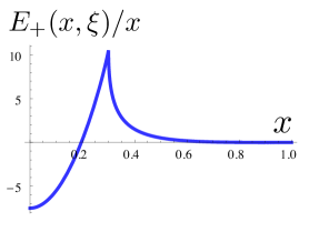
Figure 3: GPD $E_{+}(x,\xi)/x$ for $\xi=0.3$.

In a more realistic modeling, one should adjust normalization of $e(x)$ to reflect its relation to the anomalous magnetic moment. Also, the fits of the nucleon elastic form factors Guidal et al. (2005) suggest for $e(x)$ a higher power of $(1-x)$. However, our aim while showing the curves in the present paper is just to illustrate the qualitative features of various GPD models, so we will stick to the same generic forward function both for $f(x)$ and $e(x)$.

The function $E_{+}(x,\xi)$ may be displayed as

$$E_{+}(x,\xi)=x\int_{\Omega}\frac{e(\beta,\alpha)}{\beta}\left[\,\delta(x-\beta-\xi\alpha)-\delta(x-\xi\alpha)\right]\,d\beta\,d\alpha$$

$$=\int_{\Omega}e(\beta,\alpha)\,\delta(x-\beta-\xi\alpha)\,d\beta\,d\alpha$$

$$+\xi\int_{\Omega}\frac{\alpha}{\beta}\,e(\beta,\alpha)\,\left[\delta(x-\beta-\xi\alpha)-\delta(x-\xi\alpha)\right]\,d\beta\,d\alpha$$

$$=E_{DD}(x,\xi)+\xi\int_{\Omega}\left(\frac{\alpha}{\beta}\,e(\beta,\alpha)\right)_{+}\,\delta(x-\beta-\xi\alpha)\,d\beta\,d\alpha$$

$$\equiv E_{DD}(x,\xi)+{\xi}E^{1}_{+}(x,\xi)\ ,$$ (62)

where

$${E^{1}_{+}(x,\xi)}\equiv\int_{\Omega}\left(\frac{\alpha}{\beta}\,e(\beta,\alpha)\right)_{+}\,\delta(x-\beta-\xi\alpha)\,d\beta\,d\alpha\ .$$ (63)

Since $E^{1}_{+}(x,\xi)$ is built from the “plus” part of a DD, its $x$-integral from $-1$ to 1 is equal to zero, but in fact it vanishes also for a simpler reason that $E^{1}_{+}(x,\xi)$ is an odd function of $x$. So, in this case, we cannot make any conclusions about the magnitude of the $x$-integral of $E^{1}_{+}(x,\xi)$ from 0 to 1.

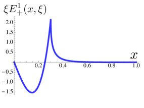
Figure 4: Function $\xi E^{1}_{+}(x,\xi)$ for $\xi=0.3$.

Summarizing, GPD $E_{+}$ is obtained from the naive $E_{DD}$ function by adding to it the $\xi E^{1}_{+}(x,\xi)$ term, which results in a rather nontrivial non-monotonic behavior of the $E_{+}$ function. To get the full GPD $E$, one should subtract also the $D$-term contribution:

$${E(x,\xi)}= E_{+}(x,\xi)-{\rm sgn}(\xi)D(x/\xi)$$ (64)

$$=E_{DD}(x,\xi)+\xi E^{1}_{+}(x,\xi)-{\rm sgn}(\xi)D(x/\xi)\ .$$

For GPD $H$, we then have

$${H(x,\xi)}=F_{DD}(x,\xi)-\xi E^{1}_{+}(x,\xi)+{\rm sgn}(\xi)D(x/\xi)\ .$$ (65)

Now one should subtract $\xi E^{1}_{+}(x,\xi)$ from the naive $F_{DD}$ function and then add the $D$-term contribution.

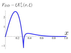
Figure 5: Model nucleon GPD $H(x,\xi)$ (without $D$-term) for $\xi=0.3$.

Comparing this result with the pion case for which

$$H(x,\xi)=F_{DD}(x,\xi)+\xi F^{1}_{+}(x,\xi)+{\rm sgn}(\xi)D(x/\xi)\ ,$$ (66)

we see that the structure of the pion GPD $H_{+}$ is similar to that of the nucleon GPD $E_{+}$: the term $\xi F^{1}_{+}(x,\xi)$ is added to $F_{DD}(x,\xi)$ rather than subtracted. However, in case of the nucleon GPD $H$, the extra term is built from the second nucleon DD $e(\beta,\alpha)$ rather than from $f(\beta,\alpha)$, and it is subtracted from $F_{DD}(x,\xi)$ rather than added to it.

V.4 Polynomiality

Taking the $x^{n}$ moment of $H(x,\xi)$ in this construction, we note that the $F_{DD}(x,\xi)$ term produces only the powers of $\xi$ up to $\xi^{n}$. Next observation is that the highest, namely $n^{\rm th}$ power of $\xi$ in the $x^{n}$ moment of $E^{1}_{+}(x,\xi)$ involves the integral

$$\int_{\Omega}\alpha^{n}\,\left(\frac{\alpha}{\beta}\,e(\beta,\alpha)\right)_{+}\,\,d\beta\,d\alpha$$ (67)

that vanishes because the integrand is a “plus” distribution with respect to $\beta$. Hence, $\xi E^{1}_{+}(x,\xi)$ term also cannot produce the $\xi^{n+1}$ contribution for the $x^{n}$ moment of $H(x,\xi)$. Such a term is produced by the $D$-term only.

V.5 Comparison with “DD plus D-term” model

The usual “DD plus D-term” model in the context of the present paper corresponds to “$F_{DD}$ plus D-term” combination, i.e. modeling nucleon GPDs without subtracting the $\xi E^{1}_{+}(x,\xi)$ term when modeling $H(x,\xi)$, (or adding it when modeling $E(x,\xi)$).

In a sense, our new model results from the old “DD plus D” model by substituting ${\rm sgn}(\xi)D(x/\xi)$ with $-\xi E^{1}_{+}(x,\xi)+{\rm sgn}(\xi)D(x/\xi)$.

Since the $D$-term is fitted to data, one may wonder if adding $\xi E^{1}_{+}(x,\xi)$ may be absorbed by redefinition of the $D$-term. However, there are important qualitative differences between $E^{1}_{+}(x,\xi)$ and $D(x/\xi)$. First, the support region of $E^{1}_{+}(x,\xi)$ is not restricted to the segment $|x|\leq\xi$. Furthermore, existing models of $D(x/\xi)$ assume that it is a continuous function that vanishes not only outside the central $|x|\leq\xi$ region, but also at the border points $|x|=\xi$ (otherwise, GPDs $H$ and $E$ would be discontinuous at the border points, and pQCD factorization formula for DVCS would make no sense). As we have seen, $E^{1}_{+}(x,\xi)$ is a continuous function of $x$ in the whole $|x|\leq 1$ region, and it is not vanishing at the border points $|x|=\xi$.

Thus, the most apparent difference between the two models is that the value of $H(\xi,\xi)$, the GPD at the border point, in the new model is different from that given by GPD $F_{DD}(\xi,\xi)$ built solely from DD $f(\beta,\alpha)$ related to the usual forward parton density $f(\beta)$. Furthermore, this difference is determined by DD $e(\beta,\alpha)$ that is related to GPD $E(x,\xi)$ invisible in the forward limit.

VI Summary

Summarizing, the model for GPD $H$ proposed in this paper differs from the “old-fashioned” DD+D model by an extra $-\xi E^{1}_{+}(x,\xi)$ term constructed from the DD $e(\beta,\alpha)$ corresponding to the GPD $E(x,\xi)$. The inclusion of such a term modifies the original DD-based term $F_{DD}(x,\xi)$ at the border points $|x|=\xi$ and outside the central $|x/\xi|\leq 1$ region, which may have strong phenomenological consequences.

References

- Mueller et al. (1994) D. Mueller, D. Robaschik, B. Geyer, F. M. Dittes, and J. Horejsi, Fortschr. Phys., 42, 101 (1994), arXiv:hep-ph/9812448 .
- Ji (1997) X.-D. Ji, Phys. Rev. Lett., 78, 610 (1997), arXiv:hep-ph/9603249 .
- Radyushkin (1996) A. V. Radyushkin, Phys. Lett., B380, 417 (1996a), arXiv:hep-ph/9604317 .
- Collins et al. (1997) J. C. Collins, L. Frankfurt, and M. Strikman, Phys. Rev., D56, 2982 (1997), arXiv:hep-ph/9611433 .
- Ji (1998) X.-D. Ji, J. Phys., G24, 1181 (1998), arXiv:hep-ph/9807358 .
- Martin and Ryskin (1998) A. D. Martin and M. G. Ryskin, Phys. Rev., D57, 6692 (1998), arXiv:hep-ph/9711371 .
- Pire et al. (1999) B. Pire, J. Soffer, and O. Teryaev, Eur. Phys. J., C8, 103 (1999), arXiv:hep-ph/9804284 .
- Radyushkin (1999) A. V. Radyushkin, Phys. Rev., D59, 014030 (1999a), arXiv:hep-ph/9805342 .
- Radyushkin (1996) A. V. Radyushkin, Phys. Lett., B385, 333 (1996b), arXiv:hep-ph/9605431 .
- Polyakov and Shuvaev (2002) M. V. Polyakov and A. G. Shuvaev, (2002), arXiv:hep-ph/0207153 .
- Polyakov (2007) M. V. Polyakov, (2007), arXiv:0711.1820 [hep-ph] .
- Polyakov (2008) M. V. Polyakov, Phys. Lett., B659, 542 (2008), arXiv:0707.2509 [hep-ph] .
- Semenov-Tian-Shansky (2008) K. M. Semenov-Tian-Shansky, Eur. Phys. J., A36, 303 (2008), arXiv:0803.2218 [hep-ph] .
- Polyakov and Semenov-Tian-Shansky (2009) M. V. Polyakov and K. M. Semenov-Tian-Shansky, Eur. Phys. J., A40, 181 (2009), arXiv:0811.2901 [hep-ph] .
- Radyushkin (1999) A. V. Radyushkin, Phys. Lett., B449, 81 (1999b), arXiv:hep-ph/9810466 .
- Polyakov and Weiss (1999) M. V. Polyakov and C. Weiss, Phys. Rev., D60, 114017 (1999), arXiv:hep-ph/9902451 .
- Goeke et al. (2001) K. Goeke, M. V. Polyakov, and M. Vanderhaeghen, Prog. Part. Nucl. Phys., 47, 401 (2001), arXiv:hep-ph/0106012 .
- Teryaev (2001) O. V. Teryaev, Phys. Lett., B510, 125 (2001), arXiv:hep-ph/0102303 .
- Belitsky et al. (2002) A. V. Belitsky, D. Mueller, and A. Kirchner, Nucl. Phys., B629, 323 (2002), arXiv:hep-ph/0112108 .
- Radyushkin (2011) A. Radyushkin, Phys.Rev., D83, 076006 (2011), arXiv:1101.2165 [hep-ph] .
- Radyushkin (2012) A. V. Radyushkin, Int.J.Mod.Phys.Conf.Ser., 20, 251 (2012).
- Szczepaniak et al. (2009) A. P. Szczepaniak, J. T. Londergan, and F. J. Llanes-Estrada, Acta Phys. Polon., B40, 2193 (2009), arXiv:0707.1239 [hep-ph] .
- Balitsky and Braun (1989) I. I. Balitsky and V. M. Braun, Nucl. Phys., B311, 541 (1989).
- Belitsky et al. (2001) A. V. Belitsky, D. Mueller, A. Kirchner, and A. Schafer, Phys. Rev., D64, 116002 (2001), arXiv:hep-ph/0011314 .
- Mankiewicz et al. (1998) L. Mankiewicz, G. Piller, and T. Weigl, Eur.Phys.J., C5, 119 (1998), arXiv:hep-ph/9711227 [hep-ph] .
- Musatov and Radyushkin (2000) I. V. Musatov and A. V. Radyushkin, Phys. Rev., D61, 074027 (2000), arXiv:hep-ph/9905376 .
- Radyushkin (2000) A. V. Radyushkin, (2000), arXiv:hep-ph/0101225 .
- Belitsky and Radyushkin (2005) A. V. Belitsky and A. V. Radyushkin, Phys. Rept., 418, 1 (2005), arXiv:hep-ph/0504030 .
- Guidal et al. (2005) M. Guidal, M. Polyakov, A. Radyushkin, and M. Vanderhaeghen, Phys.Rev., D72, 054013 (2005), arXiv:hep-ph/0410251 [hep-ph] .