On sampling SCJ rearrangement scenarios

Abstract

The Single Cut or Join ($\mathrm{SCJ}$) operation on genomes, generalizing chromosome evolution by fusions and fissions, is the computationally simplest known model of genome rearrangement. While most genome rearrangement problems are already hard when comparing three genomes, it is possible to compute in polynomial time a most parsimonious $\mathrm{SCJ}$ scenario for an arbitrary number of genomes related by a binary phylogenetic tree.

Here we consider the problems of sampling and counting the most parsimonious $\mathrm{SCJ}$ scenarios. We show that both the sampling and counting problems are easy for two genomes, and we relate $\mathrm{SCJ}$ scenarios to alternating permutations. However, for an arbitrary number of genomes related by a binary phylogenetic tree, the counting and sampling problems become hard. We prove that if a Fully Polynomial Randomized Approximation Scheme or a Fully Polynomial Almost Uniform Sampler exist for the most parsimonious $\mathrm{SCJ}$ scenario, then $\mathrm{RP}=\mathrm{NP}$.

The proof has a wider scope than genome rearrangements: the same result holds for parsimonious evolutionary scenarios on any set of discrete characters.

1 Introduction

The genome rearrangement problem is one of the oldest optimization problems in computational biology. It has been already formulated by Sturtevant and Novitski (1941). It consists in finding the minimum number of rearrangement events that can explain the gene order differences between two genomes. According to how genomes and rearrangements are defined, a number of variants have been studied (Fertin et al., 2009). In many cases, efficient algorithms running in polynomial time exist for finding one solution, but they do not scale up to three genomes: finding a median, i.e., a genome minimizing the sum of the number of rearrangements to the three others, is almost always $\mathrm{NP-hard}$.

Moreover, one solution is not representative of the whole optimal solution space. So another computational problem is to find all minimum solutions. But the number of minimum solutions is often so high that their explicit enumeration is not possible in polynomial running time. A small number of samples coming from (almost) the uniform distribution is usually sufficient for testing evolutionary hypotheses like the Random Breakpoint Model (Alekseyev and Pevzner, 2010; Bergeron et al., 2008) or the sizes and positions of inversions (Ajana et al., 2002; Darling et al., 2008). Drawing conclusions from one scenario or from a biased sample should be avoided as it might be very misleading (Bergeron et al., 2008; Miklós and Darling, 2009).

Statistical methods, like Markov chain Monte Carlo methods, can sample genome rearrangement scenarios (Darling et al., 2008; Durrett et al., 2004; Larget et al., 2002, 2005; Miklós and Tannier, 2010), but often there are no available results for their mixing time. Only in the case of the Double Cut-and-Join ($\mathrm{DCJ}$) rearrangement model, a Fully Polynomial time Randomized Approximation Scheme ($\mathrm{FPRAS}$) and a Fully Polynomial Almost Uniform Sampler ($\mathrm{FPAUS}$) are available for counting and sampling most parsimonious rearrangement scenarios between two genomes (Miklós and Tannier, 2012). But this is hardly generalizable to more than two genomes because for $\mathrm{DCJ}$ the median problem is $\mathrm{NP-hard}$ (Tannier et al., 2009).

Recently, a simpler rearrangement model has been published by Feijão and Meidanis (2011) under the name Single Cut or Join, or $\mathrm{SCJ}$. It consists in a gain and loss process on gene adjacencies, and from a chromosomal point of view, allows fusions and fissions, linearization of circular chromosomes and vice versa. The computational simplicity of this model is highlighted by the existence of an easy polynomial running time algorithm for the median problem. More generally, finding a most parsimonious $\mathrm{SCJ}$ scenario on an arbitrary evolutionary tree (the small parsimony problem) is also polynomial.

Therefore, it is reasonable to assume that at least stochastic approximations are available for the number of most parsimonious $\mathrm{SCJ}$ scenarios. We show here that it is the case for two genomes. However, we report a negative result for the small parsimony problem: the number of most parsimonious $\mathrm{SCJ}$ scenarios cannot be approximated in polynomial time even in a stochastic manner unless $\mathrm{RP}=\mathrm{NP}$. This bounds the possibilities of using this model for genomic studies.

The paper is organized as follows. The next Section formally introduces useful vocabulary in genome rearrangement and random algorithm complexity. In Section 3 we show that counting and sampling $\mathrm{SCJ}$ scenarios between two genomes is easy, and show the relation with the so-called André’s problem on alternating permutations. The hardness theorems for an arbitrary number of genomes are stated and proved in Section 4. The paper ends with a discussion on the impact of these results and the statements of some related open problems.

2 Genome rearrangement: finding, counting, sampling

2.1 Genome rearrangement by $\mathrm{SCJ}$

Definition 1.

A genome is a directed, edge-labelled graph, in which each vertex has a total degree at most 2, and each label is unique. Each edge is called a gene. The beginning of an edge is called tail, the end of an edge is called head, the joint name of heads and tails is extremities. The vertices with degree $2$ are called adjacencies, the vertices with degree $1$ are called telomeres.

By definition, a genome is a set of disjoint paths and cycles, and neither the paths nor the cycles are necessarily directed. The components of the genome are the chromosomes. An example for a couple of genomes is drawn on Figure 1.

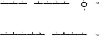
Figure 1: An example of two genomes with 9 genes.

All adjacencies correspond to two gene extremities and telomeres to one. For example, $(h1,t3)$ describes the vertex of genome $G_{2}$ in Figure 1 in which the head of gene $1$ and the tail of gene $3$ meet, and similarly, $(h7)$ is the telomere where gene $7$ ends. A genome is fully described by a list of such descriptions of adjacencies and telomeres.

We will study several genomes simultaneously. We always assume the genomes we compare have the same label set. It means they are required to have exactly the same gene content.

Definition 2.

A Single Cut or Join ($\mathrm{SCJ}$) operation transforms one genome into another by modifying the adjacencies and telomeres in one of the following $2$ ways:

• take an adjacency $(a,b)$ and replace it by two telomeres, $(a)$ and $(b)$.

• take two telomeres $(a)$ and $(b)$, and replace them by an adjacency $(a,b)$.

Given two genomes $G_{1}$ and $G_{2}$, it is always possible to transform one into the other by a sequence of $\mathrm{SCJ}$ operations (Feijão and Meidanis, 2011). Such a sequence is called an $\mathrm{SCJ}$ scenario for $G_{1}$ and $G_{2}$. Scenarios of minimum length are called most parsimonious, and their length is the $\mathrm{SCJ}$ distance and is denoted by $d_{\mathrm{SCJ}}(G_{1},G_{2})$.

The adjacency graph was introduced by Bergeron et al. (2006) to compute the $\mathrm{DCJ}$ distance between two genomes. It can be used to study $\mathrm{SCJ}$ scenarios as well:

Definition 3.

The adjacency graph $G(V_{1}\cup V_{2},E)$ of two genomes $G_{1}$ and $G_{2}$ is a bipartite multigraph in which $V_{1}$ is the set of adjacencies and telomeres of $G_{1}$ and $V_{2}$ is the set of adjacencies and telomeres of $G_{2}$. The number of edges between $u\in V_{1}$ and $v\in V_{2}$ is the number of extremities they share.

Each vertex of the adjacency graph has either degree $1$ or $2$, and thus, the adjacency graph falls into disjoint cycles and paths. Each path has one of the following three types:

• odd path, containing an odd number of edges and an even number of vertices,

• $W$-shaped path, which is an even path with two endpoints in $V_{1}$

• $M$-shaped path, which is an even path with two endpoints in $V_{2}$

In addition we call trivial components the cycles with two edges and the paths with one edge. An adjacency graph example can be seen on Figure 2.

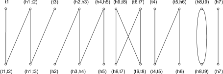
Figure 2: The adjacency graph of the two genomes on Fig. 1

2.2 Counting and Sampling $\mathrm{SCJ}$ scenarios

Definition 4.

A decision problem is in $\mathrm{NP}$ if a non-deterministic Turing Machine can solve it in polynomial time. An equivalent definition is that a witness proving the “yes” answer to the question can be verified in polynomial time. A counting problem is in $\mathrm{\#P}$ if it asks for the number of witnesses of a problem in $\mathrm{NP}$.

Definition 5.

A decision problem is in $\mathrm{RP}$ if a random algorithm exists with the following properties: a) the running time is deterministic and grows polynomially with the size of the input, b) if the true answer is “no”, then the algorithm answers “no” with probability $1$, c) if the true answer is “yes”, then it answers “yes” with probability at least $1/2$.

Definition 6.

The Most Parsimonious $\mathrm{SCJ}$ scenario problem ($\mathrm{MPSCJ}$) is to compute $d_{\mathrm{SCJ}}(G_{1},G_{2})$ for two genomes $G_{1}$ and $G_{2}$ given as input. The $\mathrm{\#MPSCJ}$ problem asks for the number of scenarios of length $d_{\mathrm{SCJ}}(G_{1},G_{2})$, denoted by $\mathrm{\#MPSCJ}(G_{1},G_{2})$.

For example, the $\mathrm{SCJ}$ distance between the two genomes of Figure 1 is $12$ and there are $16\times{12\choose 3\ 3\ 4\ 2}$ different scenarios.

$\mathrm{MPSCJ}$ is an optimization problem, which has a natural corresponding decision problem asking if there is a scenario with a given number of $\mathrm{SCJ}$ operations. So we may write that $\mathrm{\#MPSCJ}\in\mathrm{\#P}$, which means that $\mathrm{\#MPSCJ}$ asks for the number of witnesses of the decision problem “Is there a scenario for $G_{1}$ and $G_{2}$ of size $d_{\mathrm{SCJ}}(G_{1},G_{2})$ ?”.

Definition 7.

Given a rooted binary tree $T(V,E)$ with $k$ leaves, and genomes $G_{1},G_{2},\ldots,G_{k}$ assigned to the leaves, the small parsimony SCJ problem ($\mathrm{SPSCJ}$) asks for an assignment of genomes to the internal nodes of $T$ and an $\mathrm{SCJ}$ scenario for each edge, which minimize the number of $\mathrm{SCJ}$ operations along the tree, i.e.,

$$\sum_{(v_{i},v_{j})\in E}d_{\mathrm{SCJ}}(G_{i},G_{j})$$ (1)

where $G_{i}$ ($G_{j}$) is the genome which is assigned to vertex $v_{i}\in V$ ($v_{j}\in V$).

The small parsimony term is borrowed from the well-known textbook problem (Jones and Pevzner, 2004), the small parsimony problem of discrete characters: Given a rooted binary tree $T(V,E)$ with $k$ leaves labelled by characters from a finite alphabet, label the internal nodes such that the number of edges labelled with different characters at their two ends is minimized.

The solution space of the most parsimonious $\mathrm{SCJ}$ scenarios on a tree consists of all possible combinations of assignments to the internal nodes together with the possible $\mathrm{SCJ}$ scenarios on the edges of the phylogenetic tree. The $\mathrm{\#SPSCJ}$ problem asks the size of this solution space.

As the decision version of $\mathrm{SPSCJ}$ is trivially in $\mathrm{NP}$, $\mathrm{\#SPSCJ}$ is in $\mathrm{\#P}$. There are subclasses in $\mathrm{\#P}$ containing counting problems which are approximable by polynomial deterministic or randomized algorithms.

Definition 8.

A counting problem in $\mathrm{\#P}$ is in $\mathrm{FP}$ if there is a polynomial running time algorithm which gives the solution. It is $\mathrm{\#P-complete}$ if any problem in $\mathrm{\#P}$ can be reduced to it by a polynomial-time counting reduction.

Definition 9.

A counting problem in $\mathrm{\#P}$ is in $\mathrm{FPRAS}$ (Fully Polynomial Randomized Approximation Scheme) if there exists a randomized algorithm such that for any instance $x$, and $\epsilon,\delta>0$, it generates an approximation $\hat{f}$ for the solution $f$, satisfying

$$P\left(\frac{f}{1+\epsilon}\leq\hat{f}\leq f(1+\epsilon)\right)\geq 1-\delta$$ (2)

and the algorithm has a time complexity bounded by a polynomial of $|x|$, $1/\epsilon$ and $-\log(\delta)$.

The total variational distance $d_{TV}(p,\pi)$ between two discrete distributions $p$ and $\pi$ over the set $X$ is defined as

$$d_{TV}(p,\pi):=\frac{1}{2}\sum_{x\in X}|p(x)-\pi(x)|$$ (3)

Definition 10.

A counting problem in $\mathrm{\#P}$ is in $\mathrm{FPAUS}$ if there exists a randomized algorithm (a Fully Polynomial Almost Uniform Sampler that is also abbreviated as $\mathrm{FPAUS}$) such that for any instance $x$, and $\epsilon>0$, it generates a random element of the solution space following a distribution $p$ satisfying

$$d_{TV}(p,U)\leq\epsilon$$ (4)

where $U$ is the uniform distribution over the solution space, and the algorithm has a time complexity bounded by a polynomial of $|x|$, and $-\log(\epsilon)$.

3 Most parsimonious SCJ scenarios between two genomes

3.1 A dynamic programming solution

The $\mathrm{SCJ}$ distance can be calculated in polynomial time, as stated in the following theorem.

Theorem 11.

(Feijão and Meidanis (2011)) Let $\Pi_{1}$ denote the set of adjacencies in genome $G_{1}$ and let $\Pi_{2}$ denote the set of adjacencies in genome $G_{2}$. Then

$$d_{\mathrm{SCJ}}(G_{1},G_{2})=\left|\Pi_{1}\Delta\Pi_{2}\right|$$ (5)

where $\Delta$ denotes the symmetric difference of the two sets.

Theorem 11 says that any shortest path transforming $G_{1}$ into $G_{2}$ has to cut all the adjacencies in $G_{1}\setminus G_{2}$ and add all the adjacencies in $G_{2}\setminus G_{1}$, and there are no more $\mathrm{SCJ}$ operations. Drawing one solution is easy: first cut all adjacencies in $G_{1}\setminus G_{2}$, then join all adjacencies in $G_{2}\setminus G_{1}$. But if we want to explore the solution space, we have to observe that if an adjacency $(a,b)$ exists in $G_{1}\setminus G_{2}$ and an adjacency $(a,c)$ exists in $G_{2}\setminus G_{1}$, then first adjacency $(a,b)$ must be cut to create telomere $(a)$, and then telomere $(a)$ can be connected to telomere $(c)$. Similarly, if extremity $c$ belongs to an adjacency in $G_{1}\setminus G_{2}$, then it must be also cut before connecting the two telomeres. Therefore there are restrictions on the order of cuts and joins.

The allowed order of cuts and joins can be read from the adjacency graph: When an $\mathrm{SCJ}$ operation acts on $G_{1}$ and thus creates $G_{1}^{\prime}$, it also acts on the adjacency graph of $G_{1}$ and $G_{2}$ by transforming it into the adjacency graph of $G_{1}^{\prime}$ and $G_{2}$. Therefore the transformation of $G_{1}$ into $G_{2}$ can be seen as a transformation of the adjacency graph into trivial components. We say that an $\mathrm{SCJ}$ scenario sorts the adjacency graph if it transforms it into trivial components. As any $\mathrm{SCJ}$ operation in a most parsimonious scenario acts on a single component, we say that the set of $\mathrm{SCJ}$ operations acting on that component sort it if they transform it into trivial components.

We first give the way of computing the number of scenarios for sorting one component. Then the number of scenarios for several components will be deduced by a combination of scenarios from each component.

Let $W(i)$ (respectively $M(i)$, $O(i)$ and $C(i)$) denote the number of most parsimonious $\mathrm{SCJ}$ scenarios sorting a $W$-shaped path (respectively $M$-shaped path, odd path, cycle) with $i$ adjacencies in $G_{1}$. The following dynamic programming algorithm allows to compute all these numbers.

For a trivial component, no $\mathrm{SCJ}$ operation is needed so there is only one solution: the empty sequence. This gives

$$C(1) = 1$$ (6)

$$O(0) = 1$$ (7)

The smallest $W$-shaped path has 0 adjacency in $G_{1}$ and one in $G_{2}$. There is a unique solution sorting it: add the adjacency. This gives

$$W(0)=1$$ (8)

A scenario of any other component starts with cutting an adjacency in $G_{1}$. For a $W$-shaped path, this results in two $W$-shaped paths. For an $M$-shaped path, this results in two odd paths. For an odd path, this results in an odd path and a $W$-shaped path. For a cycle, this results in a $W$-shaped path. Each emerging component has fewer adjacencies in $G_{1}$, and hence, a dynamic programming recursion can be applied: the resulting components must be sorted and in case of two resulting components, the sorting steps on the components must be merged. Hence the dynamic programming recursions are

$$C(i) = i\times W(i-1)$$ (9)

$$W(i) = \sum_{j=1}^{i}{2i\choose 2j-1}W(j-1)W(i-j)$$ (10)

$$M(i) = \sum_{j=1}^{i}{2i-2\choose 2j-2}O(j-1)O(i-j)$$ (11)

$$O(i) = \sum_{j=1}^{i}{2i-1\choose 2j-2}O(j-1)W(i-j)$$ (12)

These dynamic programming recursions can be used for counting and sampling by the classical Forward-Backward phases: in the Forward phase the number of solutions is calculated, and in the Backward phase one random solution is chosen based on the numbers in the sums.

So it is possible to compute $W(i)$, $M(i)$, $O(i)$ and $C(i)$ in polynomial time and to sample one scenario from the uniform distribution. We can then count and sample for several components by adding a multinomial coefficient.

Theorem 12.

Let $G_{1}$ and $G_{2}$ be two genomes with adjacency graph $AG$. Assume $AG$ contains $i$ $M$-shaped paths, with respectively $m_{1},m_{2},\ldots,m_{i}$ adjacencies in $G_{1}$; $AG$ contains $j$ $W$-shaped paths, with respectively $w_{1},w_{2},\ldots,w_{j}$ adjacencies in $G_{1}$; $AG$ contains $k$ odd paths, with respectively $v_{1},v_{2},\ldots,v_{k}$ adjacencies in $G_{1}$; and $AG$ contains $l$ cycles, with respectively $c_{1},c_{2},\ldots,c_{l}$ adjacencies in $G_{1}$. The number of most parsimonious $\mathrm{SCJ}$ scenarios from $G_{1}$ to $G_{2}$ is

$$\frac{\left(\sum_{n=1}^{i}(2m_{n}-1)+\sum_{n=1}^{j}(2w_{n}+1)+\sum_{n=1}^{k}(2v_{n})+\sum_{n=1}^{l}(2c_{n}))\right)!}{\prod_{n=1}^{i}(2m_{n}-1)!\prod_{n=1}^{j}(2w_{n}+1)!\prod_{n=1}^{k}(2v_{n})!\prod_{n=1}^{l}(2c_{n})!} \times$$

$$\times\prod_{n=1}^{i}M(n)\prod_{n=1}^{j}W(n)\prod_{n=1}^{k}O(n)\prod_{n=1}^{l}C(n)$$ (13)

Sampling a scenario from the uniform distribution is then achieved by generating a random permutation with different colours and indices, one colour for each component, and then wipe down the indices so get a permutation with repeats. For each component, its sorting steps must be put into the joint scenario indicated by the colour of the component.

We can then state the following theorem settling the complexity of the comparison of two genomes by $\mathrm{SCJ}$.

Theorem 13.

$\mathrm{\#MPSCJ}$ is in $\mathrm{FP}$ and there is a polynomial algorithm sampling from the exact uniform distribution of the solution space of an $\mathrm{MPSCJ}$ problem.

3.2 Alternating permutations

The solutions to $\mathrm{\#MPSCJ}$ for single components are also linked to the number of alternating permutations, for which finding a formula is an old open problem. An alternating permutation of size $n$ is a permutation $c_{1},\dots,c_{n}$ of $\{1,\dots,n\}$ such that $c_{2i-1}<c_{2i}$ and $c_{2i}>c_{2i+1}$ for all $i$ (André, 1881). For example, if $n=4$, the permutation $1,3,2,4$ is an alternating permutation but $1,3,4,2$ is not because 3 is less than 4. The number of alternating permutations of size $n$ is denoted by $A_{n}$ and finding these numbers is known as André’s problem.

We show that computing $\mathrm{SCJ}$ scenarios is closely related:

Theorem 14.

$$M(k)=A_{2k-1}$$

$$W(k)=A_{2k+1}$$

$$O(k)=A_{2k}$$

$$C(k)=k\times A_{2k-1}$$

Proof.

We prove only the first line, the second and the third lines can be proved the same way. The proof of the last line comes from the fact that a cycle with $k$ adjacencies can be opened in $k$ different ways into a W-shaped component with $k-1$ adjacencies. Let the adjacencies in the $G_{1}$ part of the $M$-shaped component be $(x_{1},x_{2})$, $(x_{3},x_{4})$, $\ldots(x_{2k-1},x_{2k})$. Any $\mathrm{SCJ}$ scenario sorting these must cut all these adjacencies and must create adjacencies $(x_{2},x_{3})$, $(x_{4},x_{5})$, $\ldots(x_{2k-2},x_{2k-1})$. Let us index the $\mathrm{SCJ}$ operations in a scenario, and let $\pi_{2i-1}$ be the index of the $\mathrm{SCJ}$ step which cuts the adjacency $(x_{2i-1},x_{2i})$, and let $\pi_{2i}$ be the index of the $\mathrm{SCJ}$ step which joins $x_{2i}$ and $x_{2i+1}$.

In any most parsimonious $\mathrm{SCJ}$ sorting the $M$-shaped component, $\pi_{2i-1}<\pi_{2i}$ and $\pi_{2i+1}<\pi_{2i}$, so $\pi$ is an alternating permutation. Hence the number of sorting scenarios is at most $A_{2k-1}$.

On the other hand, for any alternating permutation of size $2k-1$, we can construct a sorting scenario in which the indexes come from the alternating permutation. Since the sorting scenarios for different alternating permutations are different, the number of $\mathrm{SCJ}$ scenarios is at least $A_{2k-1}$. ∎

4 Counting and sampling $\mathrm{SCJ}$ small parsimony solutions

The $\mathrm{SPSCJ}$ problem is in $\mathrm{P}$, since one optimal assignment of genomes to the internal nodes can be drawn in polynomial running time, (Feijão and Meidanis, 2011). However, we show that estimating the size of the solution space, as well as uniformly sampling it, is hard.

We show first that there is no polynomial running time algorithm which samples almost uniformly from the solutions unless $\mathrm{RP}=\mathrm{NP}$:

Theorem 15.

$\mathrm{\#SPSCJ}\in\mathrm{FPAUS}\Rightarrow\mathrm{RP}=\mathrm{NP}$.

Then our conjecture is that $\mathrm{\#SPSCJ}\in\mathrm{\#P-complete}$, but we can prove only a slightly weaker result

Theorem 16.

$\mathrm{\#SPSCJ}\in\mathrm{FP}\Rightarrow\mathrm{P}=\mathrm{NP}$.

Stochastic counting ($\mathrm{FPRAS}$) and sampling ($\mathrm{FPAUS}$) are equivalent for self-reducible problems [(Jerrum et al., 1986), see the quite technical definition of self-reducibility there]. However the counting counterpart of Theorem  15 cannot be immediately deduced from it because we miss a proof of self-reducibility for $\mathrm{\#SPSCJ}$, which seems far from trivial, even not true in that case. So we have to prove this counting counterpart independently.

The construction we use in the proof of Theorem 15 shows the hardness of a more specific problem and can be adapted to prove that:

Theorem 17.

$\mathrm{\#SPSCJ}\in\mathrm{FPRAS}\Rightarrow\mathrm{RP}=\mathrm{NP}$.

We first recall in the following subsection how to draw one particular solution and then how to build all possible solutions. Then we show how to generate an $\mathrm{RP}$ algorithm for $\mathrm{3SAT}$ using an $\mathrm{FPAUS}$ algorithm for the $\mathrm{\#SPSCJ}$ problem. Since $\mathrm{3SAT}\in\mathrm{NP-complete}$, this construction proves Theorem 15. This section finishes with proving Theorems 16 and 17.

4.1 The Fitch and Sankoff solutions

Let $\Pi_{1},\Pi_{2},\ldots,\Pi_{k}$ denote the adjacency sets of genomes $G_{1},G_{2},\ldots G_{k}$ and let

$$\Pi=\cup_{i=1}^{k}\Pi_{i}$$ (14)

Feijão and Meidanis (2011) proved that the parsimony score is equal to the sum of the scores for each particular adjacency $\alpha\in\Pi$. This can be computed by solving the small parsimony problem for a discrete character. Although this is mainly textbook material, we recall the principles of the standard algorithms solving this problem for one adjacency because some stages will be referred to in the hardness proof. For one adjacency, the small parsimony problem is solved by Fitch’s algorithm (Fitch, 1971). Its principle is first to assign sets ($\{0\}$, $\{1\}$ or $\{0,1\}$) to every node of the tree, visiting the nodes of the tree in post-order traversal, ie. first the leaves of the tree and then the parents of each node. At the leaves of the tree, $\{0\}$s and $\{1\}$s are assigned according to the pattern of presence or absence of $\alpha$ in the corresponding genomes. Let $B(\alpha,u)$ denote the set assigned to node $u$ regarding adjacency $\alpha$. Fitch’s algorithm applies the recursion

$$B(\alpha,u)=\begin{cases}B(\alpha,v_{1})\cap B(\alpha,v_{2})&\mbox{if }B(\alpha,v_{1})\cap B(\alpha,v_{2})\neq\emptyset\\ B(\alpha,v_{1})\cup B(\alpha,v_{2})&\mbox{otherwise}\end{cases}$$ (15)

where $v_{1}$ and $v_{2}$ are the children of $u$.

Definition 18.

We say that there is an ambiguity for an adjacency $\alpha$ at vertex $u$ if $B(\alpha,u)=\{0,1\}$.

Then starting from the root, the nodes are visited in a pre-order traversal, and $\{0\}$ or $\{1\}$ is assigned to each node according to the following rules: If $B(\alpha,\mathrm{root})$ contains only one element, then it is assigned to the root. If $B(\alpha,root)=\{0,1\}$, then any of them can be chosen for the root. Once the number assigned to the root is fixed, the values are propagated down. Let $F(\alpha,v)$ denote the singleton set assigned to the node $v$ for adjacency $\alpha$. Fitch’s algorithm applies the recursion:

$$F(\alpha,v)=\begin{cases}F(\alpha,u)\cap B(\alpha,v)&\mbox{if }F(\alpha,u)\cap B(\alpha,v)\neq\emptyset\\ B(\alpha,v)&\mbox{otherwise}\end{cases}$$ (16)

where $v$ is a child of $u$.

$F(\alpha,v)$ then always contains exactly one element. Doing this independently for all adjacencies does not guarantee that the collection of present adjacencies at each node is a genome: we call a subset $\Sigma\subseteq\Pi$ a valid genome if there is no couple of adjacencies $\alpha_{1},\alpha_{2}\in\Sigma$ with a common extremity. Feijão and Meidanis (2011) showed that if the assignments of $F(\alpha,root)$ over all possible adjacencies $\alpha\in\Pi$ are chosen to be a valid genome, then all genomes at the internal nodes are also valid (deduced from Lemmas 6.1. and 6.2 in Feijão and Meidanis (2011)). They also proved that at least one valid assignment exists since the Fitch’s algorithm never gives non-ambiguous values for adjacencies sharing extremities.

We call Fitch solutions the genome assignments constructed this way. However, they are not the only possible most parsimonious genome assignments. Some of them cannot be found by Fitch’s algorithm. All solutions can be found by a generalization of Fitch’s algorithm, Sankoff’s algorithm (Sankoff and Rousseau, 1975). It is a dynamic programming principle which computes two values for each node of the phylogenetic tree: for a leaf $v_{i}$ assigned with genome $G_{i}$,

$$s1(\alpha,v_{i})=\begin{cases}0&\mbox{if }\alpha\in\Pi_{i}\\ \infty&\mbox{otherwise}\end{cases}$$ (17)

$$s0(\alpha,v_{i})=\begin{cases}0&\mbox{if }\alpha\notin\Pi_{i}\\ \infty&\mbox{otherwise}\end{cases}$$ (18)

and for an internal node $u$ with children $v_{1}$ and $v_{2}$:

$$s1(\alpha,u) = \min\{s1(\alpha,v_{1}),s0(\alpha,v_{1})+1\}+$$ (19)

$$\min\{s1(\alpha,v_{2}),s0(\alpha,v_{2})+1\}$$

$$s0(\alpha,u) = \min\{s0(\alpha,v_{1}),s1(\alpha,v_{1})+1\}+$$ (20)

$$\min\{s0(\alpha,v_{2}),s1(\alpha,v_{2})+1\}$$

The value of $s0(\alpha,u)$ (respectively $s1(\alpha,u)$) represents the minimum number of edges under the subtree rooted at $u$ which are labelled with different presence/absence of $\alpha$ at their two ends in a most parsimonious scenario, given that $u$ is labelled with the absence (respectively presence) of $\alpha$. Then $\min(s1(\alpha,root),s0(\alpha,root))$ is the minimum small parsimony solution for adjacency $\alpha$, and the assignments to internal nodes are obtained by propagating down the values based on which gave the minimum in Equations 19 and 20.

Contrary to Fitch’s algorithm, this one explores all possible most parsimonious assignments for a given adjacency (Erdős and Székely, 1994). Unfortunately, in that case there is no guarantee that all of these assignments give valid genomes, as Feijao and Meidanis result holds only for Fitch’s solutions. It is an open question how to estimate the number of most parsimonious genome assignments (we can call them the Sankoff solutions), and is beyond the scope of this paper (note that it is a different problem from $\mathrm{\#SPSCJ}$ where we aim at estimating the number of $\mathrm{SCJ}$ scenarios and not only genome assignments).

4.2 Sampling most parsimonious $\mathrm{SPSCJ}$ scenarios is hard

In this section we construct a problem instance $x\in\mathrm{SPSCJ}$ for any $\mathrm{3CNF}$ formula $\Phi$ with $n$ variables, such that if there exists an $\mathrm{FPAUS}$ for $x$ then it is an $\mathrm{RP}$ algorithm for deciding whether or not $\Phi$ is satisfiable.

Let $\Phi$ be a $\mathrm{3CNF}$ with $n$ logical variables and $k$ clauses. We are going to construct a tree denoted by $T_{\Phi}$, and label its leaves with genomes. For each logical variable $b_{i}$ we create an adjacency $\alpha_{i}$. In this construction, all adjacencies are independent one from another, namely they never share common extremities. So there is no genome validity issue in this construction, any assignment of adjacency presence/absence is a valid genome.

For each clause $c_{j}$, we construct a subtree $T_{c_{j}}$. The construction is done in three phases, see also Figure 3. First, we create a constant size subtree, called unit subtree using building blocks we call elementary subtrees. Then in the blowing up phase, this unit subtree is repeated several times, and in the third phase it is amended with another constant size subtree. The reason for this construction is the following: the unit subtree is constructed in such a way that if a clause is satisfied, the number of $\mathrm{SCJ}$ solutions is a greater number, and is always the same number not depending on how many literals provide satisfaction of the clause. When the clause is not satisfied, the number of $\mathrm{SCJ}$ solutions is a smaller number. The blowing up is necessary for sufficiently separating the number of solutions for satisfying and not satisfying assignments. Finally, the amending is necessary for having all adjacencies ambiguous in the Fitch solutions.

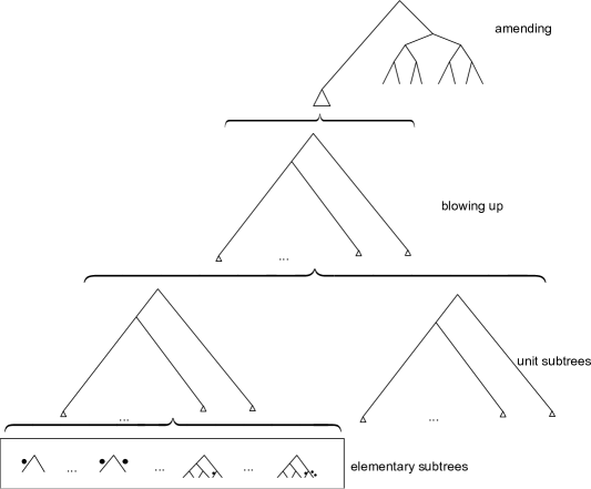
Figure 3: Constructing a subtree $T_{c_{j}}$ for a clause $c_{j}$. The subtree is built in three phases. First, elementary subtrees are connected with a comb to get a unit subtree. In the second phase the same unit subtree is repeated several times ’blowing up’ the tree. In the third phase, the blown up tree is amended with a constant size, depth 3 fully balanced tree. The smaller subtrees constructed in the previous phase are denoted with a triangle in the next phase. See also text for details.

We detail the construction of the subtree for the clause $c_{j}=b_{1}\vee b_{2}\vee b_{3}$, denoted by $T_{c_{j}}$. Subtrees for the other kinds of clauses are constructed similarly. The unit subtree is built from $76$ smaller subtrees that we will call elementary subtrees. Only $14$ different types of elementary subtrees are in a unit subtree, but several of them have given multiplicity, and the total count of them is $76$, see also Table 1. Some of the elementary subtrees are cherry motives for which we arbitrarily identify a left and a right leaf. On some of these cherries, we add one or more adjacencies, called extra adjacencies, which are present exactly on one leaf of the cherry and absent everywhere else in $T_{\Phi}$. So the edges connecting these leaves to the rest of the entire tree $T_{\Phi}$ will contain one or more additional $\mathrm{SCJ}$ operations in all most parsimonious solutions.

A clause contains $3$ logical variables, the unit subtree will be such that for the corresponding adjacencies, Fitch’s algorithm assigns an ambiguity at the root of the subtree $T_{c_{j}}$, namely

$$B(\alpha_{i},\mathrm{root})=\{0,1\}$$ (21)

for each $b_{i}\in c_{j}$. The entire tree, $T_{\Phi}$, will also be such that Sankoff solutions are all found by Fitch’s algorithm, namely, all solutions can be found by the Fitch’s algorithm, as we are going to state and prove in Lemma 20. Therefore there will be $8$ possible genome assignments for the unit subtree, related to the $8$ possible assignments of the three logical variables at the root. Let the presence of the adjacency at the root mean logical true value, and let absence mean logical false value. The constructed unit subtree will be such that if the clause is not satisfied, the number of possible $\mathrm{SCJ}$ scenarios for the corresponding assignment on this unit subtree is $2^{136}\times 3^{76}$, and if the clause is satisfied, then the number of possible $\mathrm{SCJ}$ scenarios for each corresponding assignment is $2^{156}\times 3^{64}$. The ratio of the two numbers is $2^{20}/3^{12}>1$. We will denote this number by $\gamma$. This ratio will be the basis for our proof: any $\mathrm{FPAUS}$ will sample the solutions corresponding to the satisfied clauses more often than the non-satisfied ones because the former are more numerous. This can be turned into an $\mathrm{RP}$ algorithm for $\mathrm{3SAT}$.

Below we detail the construction of the elementary subtrees and also give the number of $\mathrm{SCJ}$ solutions on them since the number of solutions on the unit subtree is simply the product of these numbers.

For the adjacencies $\alpha_{1}$, $\alpha_{2}$ and $\alpha_{3}$, the cherries are the following:

• for the cherries on which the left leaf contain one extra adjacency, the presence/absence pattern on the left and right leaf is given by
  

  $011$, $100$
  $101$, $010$
  $110$, $001$
  $000$, $111$
  

  The first column shows the presence/absence of the three adjacencies on the left leaf, the second column shows the presence/absence of the three adjacencies on the right leaf. Hence, for example, $000$ means that none of the adjacencies is present, $100$ means that only the first adjacency is present. The number of $\mathrm{SCJ}$ solutions on one cherry is $24$ if the assignment of adjacencies at the root of the cherry is the same as on the right leaf. Indeed, in that case, $4$ $\mathrm{SCJ}$ operations are necessary on the left edge, and they can be performed in any order. If the number of $\mathrm{SCJ}$ operations are $3$ and $1$ respectively on the left and right edges, or vica versa the number of solutions is $6$. Finally, if both edges have $2$ $\mathrm{SCJ}$ operations, then the number of solutions is $4$.

• There is one cherry without any extra adjacency, and its presence/absence pattern is
  

  $000$, $111$
  

  If the clause is not satisfied, the number of $\mathrm{SCJ}$ solutions on this cherry is $6$; if all logical values are true, the number of $\mathrm{SCJ}$ solutions is still $6$; in any other case, the number of $\mathrm{SCJ}$ solutions is $2$.

  This elementary subtree is repeated 3 times.

• Finally, there are cherries with one-one extra adjacency on both leaves. These are two different adjacencies, so both of them need one extra $\mathrm{SCJ}$ operation on their incoming edge. The presence/absence patterns are
  

  $011$, $100$
  $101$, $010$
  $110$, $001$
  

  If all $\mathrm{SCJ}$ operations due to $\alpha_{i}$, $i=1,2,3$ falls onto one edge, then the number of solutions is $24$, otherwise the number of solutions is $12$.

  Each of these elementary subtrees are repeated $15$ times.

The remaining elementary subtrees contain $3$ cherries connected with a comb, that is, a completely unbalanced tree, see also Figure 4. For the cherry at the right end of this elementary subtree, we add one or more adjacencies that are present on one of the leaves and absent everywhere else in $T_{\Phi}$. When there is one extra adjacency on the left leaf, the adjacencies $\alpha_{1}$, $\alpha_{2}$ and $\alpha_{3}$ are assigned with the following presences/absences on the three cherries at the top of the three combs:

$011$, $000$
$101$, $000$
$110$, $000$

Again, the first column shows the assignment for the left leaf, the second column for the right leaf. The number of $\mathrm{SCJ}$ solutions is $6$ on this cherry if the assignment at the root is $0$ for both adjacencies which has assignment $1$ on the left leaf. In any other cases, the number of solutions is $2$. Two of the adjacencies are ambiguous on this cherry, and the third one is $0$. On the remaining two cherries of this elementary subtree, this third adjacency is present on all leaves, while the other two are made ambiguous in such a way that any assignment has one $\mathrm{SCJ}$ scenario on the remaining of the tree. We show the solution for the first subtree on Figure 4.

Each of these elementary subtrees are repeated $3$ times.

Finally, there are elementary subtrees when there is $1$ extra adjacency on the left leaf and $2$ extra adjacencies on the right leaf. The assignments are

$011$, $000$
$101$, $000$
$110$, $000$

The number of $\mathrm{SCJ}$ solutions is $24$ on this cherry if both necessary $\mathrm{SCJ}$ operations fall onto the edge having $2$ additional $\mathrm{SCJ}$ operations due to the extra adjacencies, and $12$ in all other cases.

Each of these elementary subtrees are repeated $5$ times.

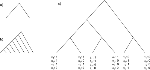
Figure 4: a) A cherry motif, ie., two leaves connected with an internal node. b) A comb, ie., a fully unbalanced tree with $8$ leaves. c) A tree with $3$ cherry motifs connected with a comb. The assignments for $4$ adjacencies, $\alpha_{1}$, $\alpha_{2}$, $\alpha_{3}$ and $\alpha_{x}$ are shown at the bottom for each leaf. $\alpha_{i}$, $i=1,2,3$ are the adjacencies related to the logical variables $b_{i}$, and $\alpha_{x}$ is an extra adjacency. Note that Fitch’s algorithm gives ambiguity for all adjacencies $\alpha_{i}$ at the root of this subtree.

	011	101	110	000	011	101	110	000	011	101	110	011	101	110
#	1	1	1	1	3	3	3	3	5	5	5	15	15	15
000	6	6	6	6	$6^{3}$	$6^{3}$	$6^{3}$	$6^{3}$	$12^{5}$	$12^{5}$	$12^{5}$	$12^{15}$	$12^{15}$	$12^{15}$
100	24	4	4	4	$6^{3}$	$2^{3}$	$2^{3}$	$2^{3}$	$12^{5}$	$12^{5}$	$12^{5}$	$24^{15}$	$12^{15}$	$12^{15}$
010	4	24	4	4	$2^{3}$	$6^{3}$	$2^{3}$	$2^{3}$	$12^{5}$	$12^{5}$	$12^{5}$	$12^{15}$	$24^{15}$	$12^{15}$
110	6	6	6	6	$2^{3}$	$2^{3}$	$2^{3}$	$2^{3}$	$12^{5}$	$12^{5}$	$24^{5}$	$12^{15}$	$12^{15}$	$24^{15}$
001	4	4	24	4	$2^{3}$	$2^{3}$	$6^{3}$	$2^{3}$	$12^{5}$	$12^{5}$	$12^{5}$	$12^{15}$	$12^{15}$	$24^{15}$
101	6	6	6	6	$2^{3}$	$2^{3}$	$2^{3}$	$2^{3}$	$12^{5}$	$24^{5}$	$12^{5}$	$12^{15}$	$24^{15}$	$12^{15}$
011	6	6	6	6	$2^{3}$	$2^{3}$	$2^{3}$	$2^{3}$	$24^{5}$	$12^{5}$	$12^{5}$	$24^{15}$	$12^{15}$	$12^{15}$
111	4	4	4	24	$2^{3}$	$2^{3}$	$2^{3}$	$6^{3}$	$24^{5}$	$24^{5}$	$24^{5}$	$12^{15}$	$12^{15}$	$12^{15}$

Table 1: The number of $\mathrm{SCJ}$ scenarios on different elementary subtrees of the unit subtree of the subtree $T_{c_{j}}$ for clause $c_{j}=b_{1}\vee b_{2}\vee b_{3}$. Columns represent the $14$ different types of components, the topology of the elementary subtree is indicated on the top. The black dot means extra $\mathrm{SCJ}$ operations on the indicated edge, the numbers represent the presence/absence of adjacencies on the left leaf of a particular cherry, see text for details. The row starting with # indicates the number of repeats of the elementary subtrees. Further rows represent the logical true/false values of $b_{i}$s, for example, $001$ means $b_{1}=false$, $b_{2}=false$, $b_{3}=true$. The values in the table indicate the number of solutions, raised to the appropriate power due to multiplicity of the elementary subtrees. It is easy to check that the product of the numbers in the first line is $2^{136}\times 3^{76}$ and in any other lines is $2^{156}\times 3^{64}$.

In this way, the roots of all 76 elementary subtrees are ambiguous for the three adjacencies related to logical variables. We connect the 76 elementary subtrees with a comb, and thus, all three adjacencies are ambiguous at the root of the entire subtree, which is the unit subtree. If the clause is satisfied, the number of SCJ scenarios for the corresponding assignment is $2^{156}\times 3^{64}$, if the clause is not satisfied, the number of SCJ solutions is $2^{136}\times 3^{76}$, as can be checked on Table 1. The ratio of them is indeed $2^{20}/3^{12}=\gamma$. The number of leaves on this unit subtree is $248$, and $148$ additional adjacencies are introduced.

This was the construction of the constant size unit subtree. In the next step, we “blow up” the system. Similar blowing up can be found in Jerrum et al. (1986), in the proof of Theorem 5.1. We repeat the above described unit subtree $\left\lceil(k\log((n-3)!)+n\log(2))/\log(\gamma)\right\rceil+1$ times, and connect all of them with a comb (completely unbalanced tree). All three adjacencies representing the three logical variables in the clause are still ambiguous at the root of this blown up subtree, and thus, there are still $8$ Fitch solutions. For a solution satisfying the clause, the number of $\mathrm{SCJ}$ scenarios on this blown up subtree is

$$X=\left(2^{156}\times 3^{64}\right)^{\left\lceil\frac{k\log((n-3)!)+n\log(2)}{\log(\gamma)}\right\rceil+1}$$ (22)

and the number of scenarios if the clause is not satisfied is

$$Y=\left(2^{136}\times 3^{76}\right)^{\left\lceil\frac{k\log((n-3)!)+n\log(2)}{\log(\gamma)}\right\rceil+1}$$ (23)

Let all adjacencies not participating in the clause be $0$ on this blown up subtree.

We are close to the final subtree $T_{c_{j}}$ for one clause, $c_{j}$. In the third phase, we amend the so far obtained tree with a constant size subtree. Construct a fully balanced depth $3$ binary tree, on which all $3$ adjacencies which are in the clause are ambiguous at the root without making more than $1$ $\mathrm{SCJ}$ scenario on it, similarly to the left part of the tree on Figure 4. All other adjacencies not participating in the clause are present at all leaves of this tree.

Here is how to construct $T_{c_{j}}$ for one clause, $c_{j}$. Construct an additional vertex which will be its root. The left child of the root is the blown up tree, while its right child is the depth $3$ balanced tree. Denote by $T_{c_{j}}$ this final tree for one clause $c_{j}$.

All adjacencies are ambiguous at the root of the subtree $T_{c_{j}}$, therefore there are $2^{n}$ Fitch solutions for the assignments of the internal nodes of $T_{c_{j}}$.

Lemma 19.

For any assignment of the $n$ adjacencies, if the clause $c_{i}$ is satisfied, then the number of $\mathrm{SCJ}$ scenarios for the corresponding assignment on $T_{c_{j}}$ is at least

$$Y\times((n-3)!)^{k}\times 2^{n}\times\gamma$$ (24)

and at most

$$Y\times((n-3)!)^{k+1}\times 2^{n}\times\gamma$$ (25)

If the clause is not satisfied, then the number of $\mathrm{SCJ}$ scenarios is at most $Y\times(n-3)!$.

Proof.

The $B$ values of Fitch’s algorithm for the $n-3$ adjacencies not representing a logical value in the clause $c_{i}$ are all $\{0\}$ at all the nodes of the left child of the root, and all $\{1\}$ at all the nodes of the right child of the root. Therefore in all scenarios there are $n-3$ cumulated $\mathrm{SCJ}$ operations on the two edges going out of the root. If they are all on one of the edges, the number of possible $\mathrm{SCJ}$ scenarios is $(n-3)!$, and in all other cases they are less, but at least $1$. (Actually, the minimum is $\left(((n-3)/2)!\right)^{2}$, but the very loose lower bound $1$ is sufficent for our calculations). Then if the clause is satisfied, the number of $\mathrm{SCJ}$ scenarios is between $X$ and $X\times(n-3)!$. Note that

$$X/Y=((n-3)!)^{k}\times 2^{n}\times\gamma,$$

which gives the stated result. If the clause is not satisfied, the number of $\mathrm{SCJ}$ scenarios is at most $Y\times(n-3)!$. ∎

For all $k$ clauses, construct such a subtree and connect all of them with a comb. This is the final tree $T_{\Phi}$ for the $\mathrm{3CNF}$ $\Phi$.

All adjacencies corresponding to logical variables are ambiguous at the root of the $T_{\Phi}$, so there are $2^{n}$ Fitch solutions. We prove that there is the same number of Sankoff solutions.

Lemma 20.

All adjacency assignments for the $\mathrm{SPSCJ}$ problem on tree $T_{\Phi}$ are Fitch solutions.

Proof.

There are two types of adjacencies participating in $T_{\Phi}$. There are $n$ of them related to the logical variables in $\Phi$, the other adjacencies are introduced in the construction and are present on exactly one leaf, absent everywhere else in $T_{\Phi}$.

If an adjacency $\alpha_{x}$ is present only on one leaf, then in any $\mathrm{SPSCJ}$ solution it is created on the edge connecting the leaf to the remaining part of the tree. This solution is provided by Fitch’s algorithm.

The tree is constructed in such way that for all $\alpha_{i}$ representing variable $b_{i}\in\Phi$,

$$B(\alpha_{i},v)=\{0,1\}\Rightarrow B(\alpha_{i},u)=\{0,1\}$$ (26)

where $u$ is the parent of $v$. First observe that

$$B(\alpha_{i},v)=\{0,1\}\Rightarrow s1(\alpha_{i},u)=s0(\alpha_{i},u)$$ (27)

this means that whenever the two children $v_{1}$ and $v_{2}$ of a node $u$ are ambiguous in Fitch’s algorithm,

$$s1(\alpha_{i},u) = s1(\alpha_{i},v_{1})+s1(\alpha_{i},v_{2})$$ (28)

$$s0(\alpha_{i},u) = s0(\alpha_{i},v_{1})+s0(\alpha_{i},v_{2})$$ (29)

namely, all Sankoff solutions are Fitch solutions.

Moreover, at any node $u$ where the $B$ value is ambiguous for some adjacency $\alpha_{i}$, while it is not ambiguous in the children of $u$, we have

$$s0(\alpha_{i},u)=s1(\alpha_{i},u)=1$$ (30)

and here again the Fitch solutions are the same as the Sankoff solutions. ∎

Now we are ready to prove Theorem 15.

Proof.

(Theorem 15.) Let $\Phi$ be a $\mathrm{3CNF}$ with $k$ clauses. The number of Boolean variables in $\Phi$ is at most $3k$, hence the tree $T_{\Phi}$ contains at most

$$\left(248\times\left(\left\lceil\frac{k\log((3k-3)!)+3k\log(2)}{\log(\gamma)}\right\rceil+1\right)+8\right)\times k$$ (31)

leaves, and

$$6k+296k\times\left(\left\lceil\frac{k\log((3k-3)!)+3k\log(2)}{\log(\gamma)}\right\rceil+1\right)$$ (32)

extremities (twice the number of independent adjacencies appearing). To explain Equation 31, $248$ is the number of leaves on the unit subtree, it is reapeted $\left\lceil\frac{k\log((n-3)!)+3k\log(2)}{\log(\gamma)}\right\rceil+1$ times, an upper bound for $n$ is $3k$, as mentioned above, and there are $8$ further leaves in the amending phase of the construction of a subtree $T_{c_{j}}$ for a clause $c_{j}$. Finally, there are $k$ clauses. To explain Equation 32, there is an adjacency for each boolean variable, there are at most $3k$ of them, each of them having $2$ extremities, yielding $6k$ extremities at most. There are $148$ extra adjacencies in each unit subtree, having $296$ extremities. Each unit subtree is repeated $\left\lceil\frac{k\log((n-3)!)+3k\log(2)}{\log(\gamma)}\right\rceil+1$ times, upperly bounded by $\left\lceil\frac{k\log((3k-3)!)+3k\log(2)}{\log(\gamma)}\right\rceil+1$, and this is done for each $k$ clauses.

Hence the input size for the $\mathrm{SPSCJ}$ problem is a polynomial function of the size of $\Phi$.

If $\Phi$ is satisfiable, then there exists an assignment for which the number of $\mathrm{SCJ}$ scenarios is at least

$$Y^{k}\times(((n-3)!)^{k}\times 2^{n}\times\gamma)^{k}$$ (33)

If at least one of the clauses is not satisfied, then the total number of $\mathrm{SCJ}$ scenarios is at most

$$Y^{k}\times(((n-3)!)^{k}\times 2^{n}\times\gamma)^{k-1}\times\left((n-3)!\right)^{k}$$ (34)

Therefore, if $\Phi$ is satisfiable, there are at most $2^{n}-1$ assignments which do not satisfy the $\Phi$, and the number of corresponding $\mathrm{SCJ}$ scenarios is at most

$$Y^{k}\times(((n-3)!)^{k}\times 2^{n}\times\gamma)^{k-1}\times\left((n-3)!\right)^{k}\times(2^{n}-1).$$ (35)

Hence if $\Phi$ is satisfiable, then the number of $\mathrm{SCJ}$ scenarios related to satisfying assignments are more than the number of other $\mathrm{SCJ}$ scenarios. If an $\mathrm{FPAUS}$ exists for all most parsimonious scenarios, then it would sample satisfying scenarios with more than $0.5$ probability. Then this is an $\mathrm{RP}$ algorithm for $\mathrm{3SAT}$. An $\mathrm{RP}$ algorithm for $\mathrm{3SAT}$ immediately implies that $\mathrm{RP}=\mathrm{NP}$ (Papadimitriou, 1993). ∎

4.3 Counting problems

The same construction is sufficient to prove Theorem 16.

Proof.

(Theorem 16.) Assume that there is an $\mathrm{FP}$ algorithm for $\mathrm{\#SPSCJ}$. Then for any $\mathrm{3CNF}$ $\Phi$, construct the above introduced problem instance $x\in\mathrm{\#SPSCJ}$, and calculate the exact number of solutions. If $\Phi$ is not satisfiable, then the number of solutions is at most

$$Y^{k}\times(((n-3)!)^{k}\times 2^{n}\times\gamma)^{k-1}\times\left((n-3)!\right)^{k}\times 2^{n}$$ (36)

If $\Phi$ can be satisfied, then the number of solutions is more than

$$Y^{k}\times(((n-3)!)^{k}\times 2^{n}\times\gamma)^{k}$$ (37)

Since the number in Equation 37 is greater than the number in Equation 36, and the number of digits of these numbers grows only polynomially with $|\Phi|$, given an $\mathrm{FP}$ algorithm for $\mathrm{\#SPSCJ}$, it would be decidable in polynomial running time whether or not $\Phi$ is satisfiable. Since $\mathrm{3SAT}\in\mathrm{NP-complete}$, it would imply that $\mathrm{P}=\mathrm{NP}$. ∎

Now we prove the counting counterpart of the same result, that is, $\mathrm{\#SPSCJ}$ is not in $\mathrm{FPRAS}$ unless $\mathrm{RP}=\mathrm{NP}$. For this we need to define a more restricted problem.

Definition 21.

The $\mathrm{\#Fitch-SPSCJ}$ problem asks for the number of Fitch solutions of an $\mathrm{SPSCJ}$ instance where pairs of adjacencies never share an extremity and the values of a set of ambiguous adjacencies are fixed.

Although stricto sensu, the $\mathrm{\#Fitch-SPSCJ}$ is still not a self reducible counting problem, we can prove that it has an $\mathrm{FPAUS}$ algorithm if it has an $\mathrm{FPRAS}$ algorithm. Before proving it, we discuss in a nutshell how to construct an $\mathrm{FPAUS}$ algorithm from an $\mathrm{FPRAS}$ algorithm for self-reducible counting problems. The description is not detailed, for a strict mathematical description, see Sinclair (1992).

The heart of the method that creates an $\mathrm{FPAUS}$ from a self-reducible counting problem in $\mathrm{FPRAS}$ is a rejection sampler (von Neumann, 1951). A random solution is drawn sequentially travelling down the counting tree of the self-reducible problem, using the $\mathrm{FPRAS}$ approximations for the children of the current node, and at each internal node the sampling probability is calculated. The sampling probabilities are used to calculate the so called rejection rate, the probability that the sample will be rejected. The central theorem of the rejection method states that the accepted samples come from sharp the uniform distribution. To transform this into an $\mathrm{FPAUS}$, the rejection rate should be relatively small, so in a few (polynomial number of) trials, the probability that all trials are rejected becomes negligible. If all trials are rejected, then an arbitrary solution is drawn, but due to its extremely small probability, it causes a very small deviation from the uniform distribution (measured in variational distance).

Lemma 22.

$\mathrm{\#Fitch-SPSCJ}\in\mathrm{FPRAS}\Rightarrow\mathrm{\#Fitch-SPSCJ}\in\mathrm{FPAUS}$

Proof.

It is sufficient to show that the solutions can be put onto a counting tree such that the depth of the tree is $O(poly(|x|))$ where $|x|$ is the size of the problem instance, and for any internal node, one of the following is true:

• The number of descendants of the internal node is $O(poly(|x|))$ where $|x|$ is the size of the problem instance, and for each descendant, a problem $x^{\prime}\in\mathrm{\#Fitch-SPSCJ}$ exists whose number of solutions is the number of leaves of that tree, and $|x^{\prime}|=O(poly(|x|))$.

• The number of descendants is $O(c^{poly(|x|)})$ for some $c>1$, but a perfect sampler exists that can sample sharp the uniform distribution of the descendants and the number of descendants can be calculated, both the sampler and the counter run in $O(poly(|x|))$ time. Furthermore, all descendants are leaves.

The algorithms in the second case provide that the protocol constructing an $\mathrm{FPAUS}$ sampler using an $\mathrm{FPRAS}$ algorithm described briefly above can be done also for those nodes which have suprapolynomial number of descendants but counting their number as well as sharp uniform sampling them can be done in polynomial time. Indeed, both sampling and calculating the sampling probabilities can be done in polynomial running time, and it is easy to see that the strict uniform sampling does not increase the rejection rate.

Fix an arbitrary total ordering of adjacencies. Let $u$ be an internal node, and $z$ is the associated problem to it. If there are ambiguities at the root of the evolutionary tree, then take the smallest adjacency with ambiguity and without a constraint, let it be denoted by $\alpha$. Then $u$ will have two descendants, and they are associated with a problem instance where problem instance $z$ is modified such that $\alpha$ has constraint $0$ and constraint $1$.

If $z$ does not have any ambiguity, then its assignment is unique. For this unique assignment, the number of $\mathrm{SCJ}$ scenarios along each edge can be counted and sharply uniformly sampled (Theorem 13), so these will be the descendants of $u$ and also the leaves below $u$. ∎

The next lemma leads directly to the proof of Theorem 17.

Lemma 23.

$\mathrm{\#SPSCJ}\in\mathrm{FPRAS}\Rightarrow\mathrm{\#Fitch-SPSCJ}\in\mathrm{FPRAS}$

Proof.

Let $x$ be a problem instance from $\mathrm{\#Fitch-SPSCJ}$. Let $A$ denote the set of adjacencies which are ambiguous at the root, but there are constraints on them. Let $T$ denote the evolutionary tree of the problem instance $x$.

We construct another problem $x^{\prime}$, which has the same number of $\mathrm{SCJ}$ solutions but there are no ambiguities for those adjacencies which are in $A$. We remove each $\alpha\in A$, and introduce new, independent adjacencies. For any $\alpha\in A$, let $E(\alpha)$ denote the set of edges of $T$ for which an SCJ operation is necessary with the prescribed assignment of $\alpha$. We introduce $|E(\alpha)|$ new, independent adjacencies in the following way. For each $e\in E(\alpha)$, if $\alpha$ is generated on the edge, then let the corresponding adjacency $\alpha_{e}$ be present at the leaves below edge $e$, and nowhere else. Otherwise, if $\alpha$ is cut along the edge $e$, let the corresponding adjacency $\alpha_{e}$ be absent at the leaves below edge $e$, and be present at all other leaves. It is easy to see that the only most parsimonious solution for $\alpha_{e}$ is to create or cut $\alpha_{e}$ with an SCJ operation along edge $e$. Clearly, $x\in\mathrm{\#SPSCJ}$, as there are no constraints on its adjacencies, the number of solutions for $x^{\prime}$ is the same as the number of solutions for $x$, moreover

$$|x^{\prime}|=O(|x|+|A|\times|T|).$$ (38)

Therefore an $\mathrm{FPRAS}$ algorithm for $x^{\prime}$ is also an $\mathrm{FPRAS}$ for $x$. ∎

We can now prove Theorem 17.

Proof.

(Theorem 17). From Lemma 23

$$\mathrm{\#SPSCJ}\in\mathrm{FPRAS}\Rightarrow\mathrm{\#Fitch-SPSCJ}\in\mathrm{FPRAS}$$ (39)

From Lemma 22,

$$\mathrm{\#Fitch-SPSCJ}\in\mathrm{FPRAS}\Rightarrow\mathrm{\#Fitch-SPSCJ}\in\mathrm{FPAUS}$$ (40)

Putting these together, we get that

$$\mathrm{\#SPSCJ}\in\mathrm{FPRAS}\Rightarrow\mathrm{\#Fitch-SPSCJ}\in\mathrm{FPAUS}$$ (41)

But from the proof of Theorem 15. It is clear that an $\mathrm{FPAUS}$ already for $\mathrm{\#Fitch-SPSCJ}$ would imply that $\mathrm{RP}=\mathrm{NP}$. ∎

5 Discussion/Conclusions

We proved non-approximability for a counting problem motivated by computational biology, whose optimization/decision counterpart problem is in $\mathrm{P}$.

The problem is related to the evolution of discrete characters: imagine a set of $n$ independent characters from a finite set (a nucleotide sequence where all nucleotides evolve independently for instance), and a set of species related by a binary phylogenetic tree. The values of the $n$ characters are known at the leaves, and the small parsimony problem asks for assignments at the internal nodes of the tree. Here finding one most parsimonious assignment is easy, but it is also easy to count their number or sample them uniformly, when they are all independent, which is not the case for adjacencies in genomes. However, if the assignments are weighted by the number of most parsimonious evolutionary scenarios on the whole set of characters, then there is no possible efficient counting or sampling method. Indeed, in our proof all adjacencies are independent, so it applies to this more general problem.

This study also highlights a counting bias in the parsimony $\mathrm{SCJ}$ model with independent adjacencies (or evolutionary scenarios on discrete characters). For example, take a cherry with ambiguous values at its root. The number of scenarios is higher if the assignment at the root of the cherry is equal to one of the leaves than if it is a mix between the two. In an unbiased model all assignments should be equiprobable. This observation leads to two possible directions for future work:

• Counting assignments. If all assignments should be equiprobable, then the problem is to count and sample in the assignment solution space. It is our unpublished result that counting the number of Fitch solutions to $\mathrm{SPSCJ}$ is in $\mathrm{FP}$, but counting the Sankoff type assignments has an unknown computational complexity.

• Probabilistic models. The bias of the parsimony model will drop in a probabilistic approach. Here mutations follow a continuous time Markov model. In that case, each potential $\mathrm{SCJ}$ operation has an exponential waiting time for the occurrence. The so-called trajectory likelihood can be calculated analytically, see Miklós et al. (2004). The sum of the trajectory likelihoods is the total likelihood of two genomes, i.e., what is the probability that genome $G_{1}$ becomes genome $G_{2}$ after time $t$, given a set of parameters for the exponential distributions put onto the potential $\mathrm{SCJ}$ operations. The total likelihood calculation has an unknown computational complexity.

  We can also consider the probabilistic approach on a tree. In case of independent events, it can be shown that the multinomial coefficients describing how many combinations exist to merge the independent $\mathrm{SCJ}$ operations are cancelled out in the likelihood calculations. If all edge lengths of the evolutionary tree are the same, and all adjacencies are independent, then the probabilistic $\mathrm{\#SPSCJ}$ problem reduces to counting the assignments to the internal nodes of the evolutionary tree, which might have a simpler computational complexity.

These are promising future directions of research, which can be important for comparative genomics. To close the mathematical aspects of the $\mathrm{SPSCJ}$ problem, two unsolved questions remain:

• $\mathrm{\#P}$-completness of $\mathrm{\#SPSCJ}$. Our conjecture is that $\mathrm{\#SPSCJ}\in\mathrm{\#P-complete}$. Theorem 16 strengthens this conjecture. Although $\mathrm{\#3SAT}\in\mathrm{\#P-complete}$, the construction in the proof of Theorem 15 is not sufficient for counting the number of satisfying assignments of $\Phi$. For each satisfying assignment, there is a multiplicative coefficient that can vary between $\left(\frac{n-3}{2}\right)!^{2}$ and $(n-3)!$, and this shadows the exact number of solutions.

• Star tree problem. Given a set of genomes, $G_{1},G_{2},\ldots G_{k}$ related to a star tree, count and sample their most parsimonious $\mathrm{SCJ}$ scenarios. If $k$ is odd, then the assignment for the centre of the star tree is unique. It is proved for the median genome of $3$ genomes by Feijão and Meidanis (2011), and their proof can be extended to any odd number of genomes. However, when $k$ is even, then the median might not be unique, and there might be exponentially many solutions for the assignment. The computational complexity for this case is an open question. This generalizes to the small parsimony problem on non-binary trees.

6 Acknowledgments

I.M. was supported by OTKA grant PD84297. S.Z.K. was supported by OTKA grants K77476 and NK 105645.

References

- Ajana et al. (2002) Ajana, Y., Lefebvre, J., Tillier, E., El-Mabrouk., N., 2002. Exploring the set of all minimal sequences of reversals - an application to test the replication-directed reversal hypothesis. In: Algorithms in Bioinformatics (WABI’02). Vol. 2452 of LNCS. pp. 300–315.
- Alekseyev and Pevzner (2010) Alekseyev, M. A., Pevzner, P. A., 2010. Comparative genomics reveals birth and death of fragile regions in mammalian evolution. Genome Biol 11 (11), R117.
- André (1881) André, D., 1881. Mémoire sur les permutations alternées. Journal de mathématiques pures et appliquées 7, 167––184.
- Bergeron et al. (2006) Bergeron, A., Mixtacki, J., Stoye, J., 2006. A unifying view of genome rearrangements. LNCS 4175, 163–173.
- Bergeron et al. (2008) Bergeron, A., Mixtacki, J., Stoye, J., 2008. On computing the breakpoint reuse rate in rearrangement scenarios (preview). In: Proceedings of RECOMB-CG 2008. Vol. 5267 of LNBI. pp. 226–240.
- Darling et al. (2008) Darling, A., Miklós, I., Ragan, M., 2008. Dynamics of genome rearrangement in bacterial populations. PLoS Genetics 4 (7), e1000128.
- Durrett et al. (2004) Durrett, R., Nielsen, R., York, T., 2004. Bayesian estimation of genomic distance. Genetics 166, 621–629.
- Erdős and Székely (1994) Erdős, P. L., Székely, L. A., 1994. On weighted multiway cuts in trees. Mathematical Programming 65, 93–105.