The correlation structure of local neuronal networks intrinsically results from recurrent dynamics

Moritz Helias¹, Tom Tetzlaff¹, Markus Diesmann^1,2

¹ Institute of Neuroscience and Medicine (INM-6) and Institute for Advanced Simulation (IAS-6), Jülich Research Centre and JARA, Jülich, Germany

² Medical Faculty, RWTH Aachen University, Aachen, Germany

                                                                                                           
Correspondence to:    Dr. Moritz Helias tel: +49-2461-61-9467 m.helias@fz-juelich.de

Abstract

Correlated neuronal activity is a natural consequence of network connectivity and shared inputs to pairs of neurons, but the task-dependent modulation of correlations in relation to behavior also hints at a functional role. Correlations influence the gain of postsynaptic neurons, the amount of information encoded in the population activity and decoded by readout neurons, and synaptic plasticity. Further, it affects the power and spatial reach of extracellular signals like the local-field potential. A theory of correlated neuronal activity accounting for recurrent connectivity as well as fluctuating external sources is currently lacking. In particular, it is unclear how the recently found mechanism of active decorrelation by negative feedback on the population level affects the network response to externally applied correlated stimuli. Here, we present such an extension of the theory of correlations in stochastic binary networks. We show that (1) for homogeneous external input, the structure of correlations is mainly determined by the local recurrent connectivity, (2) homogeneous external inputs provide an additive, unspecific contribution to the correlations, (3) inhibitory feedback effectively decorrelates neuronal activity, even if neurons receive identical external inputs, and (4) identical synaptic input statistics to excitatory and to inhibitory cells increases intrinsically generated fluctuations and pairwise correlations. We further demonstrate how the accuracy of mean-field predictions can be improved by self-consistently including correlations. As a byproduct, we show that the cancellation of correlations between the summed inputs to pairs of neurons does not originate from the fast tracking of external input, but from the suppression of fluctuations on the population level by the local network. The suppression of fluctuations on the population level is a necessary constraint, but not sufficient to determine the structure of correlations. Therefore, the structure of correlations does not follow from the fast tracking of external inputs.

Author summary

The co-occurrence of action potentials of pairs of neurons within short time intervals is known since long. Such synchronous events can appear time-locked to the behavior of an animal and also theoretical considerations argue for a functional role of synchrony. Early theoretical work tried to explain correlated activity by neurons transmitting common fluctuations due to shared inputs. This, however, overestimates correlations. Recently the recurrent connectivity of cortical networks was shown responsible for the observed low baseline correlations. Two different explanations were given: One argues that excitatory and inhibitory population activities closely follow the external inputs to the network, so that their effects on a pair of cells mutually cancel. Another explanation relies on negative recurrent feedback to suppress fluctuations in the population activity, equivalent to small correlations. In a biological neuronal network one expects both, external inputs and recurrence, to affect correlated activity. The present work extends the theoretical framework of correlations to include both contributions and explains their qualitative differences. Moreover the study shows that the arguments of fast tracking and recurrent feedback are not equivalent, only the latter correctly predicts the cell-type specific correlations.

Introduction

The spatio-temporal structure and magnitude of correlations in cortical neural activity have since long been subject of research for a variety of reasons: The experimentally observed task-dependent modulation of correlations points at a potential functional role. In the motor cortex of behaving monkeys, for example, synchronous action potentials appear at behaviorally relevant time points [32]. The degree of synchrony is modulated by task performance, and the precise timing of synchronous events follows a change of the behavioral protocol after a phase of re-learning. In primary visual cortex, saccades (eye movements) are followed by brief periods of synchronized neural firing [37, 28]. Further, correlations and fluctuations depend on the attentive state of the animal [11], with higher correlations and slow fluctuations observed during quiet wakefulness, and faster, uncorrelated fluctuations in the active state [48]. It is still unclear whether the observed modulation of correlations is in fact employed by the brain, or whether it is merely an epiphenomenon. Theoretical studies have suggested a number of interpretations and mechanisms of how correlated firing could be exploited: Correlations in afferent spike-train ensembles may provide a gating mechanism by modulating the gain of postsynaptic cells (for a review, see [53]). Synchrony in afferent spikes (or, more generally, synchrony in spike arrival) can enhance the reliability of postsynaptic responses and, hence, may serve as a mechanism for a reliable activation and propagation of precise spatio-temporal spike patterns [1, 13, 29, 57]. Further, it has been argued that synchronous firing could be employed to combine elementary representations into larger percepts [22, 65, 1, 5, 55]. While correlated firing may constitute the substrate for some en- and decoding schemes, it can be highly disadvantageous for others: The number of response patterns which can be triggered by a given afferent spike-train ensemble becomes maximal if these spike trains are uncorrelated [60]. In addition, correlations in the ensemble impair the ability of readout neurons to decode information reliably in the presence of noise (see e.g. [66, 60, 58]). Recent studies have indeed shown that biological neural networks implement a number of mechanisms which can efficiently decorrelate neural activity, such as the nonlinearity of spike generation [12], synaptic-transmission variability and failure [50, 51], short-term synaptic depression [51], heterogeneity in network connectivity [3] and neuron properties [42]and the recurrent network dynamics [24, 49, 58]. To study the significance of experimentally observed task-dependent correlations, it is essential to provide adequate null hypotheses: Which level and structure of correlations is to be expected in the absence of any task-related stimulus or behavior? Even in the simplest network models without time varying input, correlations in the neural activity emerge as a consequence of shared input [54, 59, 33] and recurrent connectivity [49, 45, 58, 61, 23]. Irrespective of the functional aspect, the spatio-temporal structure and magnitude of correlations between spike trains or membrane potentials carry valuable information about the properties of the underlying network generating these signals [59, 45, 46, 61, 23] and could therefore help constraining models of cortical networks. Further, the quantification of spike-train correlations is a prerequisite to understand how correlation sensitive synaptic plasticity rules, such as spike-timing dependent plasticity [4], interact with the recurrent network dynamics [17]. Finally, knowledge of the expected level of correlations between synaptic inputs is crucial for the correct interpretation of extracellular signals like the local-field potential (LFP) [34].

Previous theoretical studies on correlations in local cortical networks provide analytical expressions for the magnitude [33, 49, 58] and the temporal shape [18, 38, 61, 23] of average pairwise correlations, capture the influence of the connectivity on correlations [35, 41, 45, 46, 61, 27], and connect oscillatory network states emerging from delayed negative feedback [8] to the shape of correlation functions [23]. We have in particular shown recently that negative feedback loops, abundant in cortical networks, constitute an efficient decorrelation mechanism and therefore allow neurons to fire nearly independently despite substantial shared presynaptic input [58] (see also [35, 49, 36]). We further pointed out that in networks of excitatory (E) and inhibitory (I) neurons, the correlations between neurons of different cell type (EE, EI, II) differ in both magnitude and temporal shape, even if excitatory and inhibitory neurons have identical properties and input statistics [58, 23]. It remains unclear, however, how this cell-type specificity of correlations is affected by the connectivity of the network.

The majority of previous theoretical studies on cortical circuits is restricted to local networks driven by external sources representing thalamo-cortical or cortico-cortical inputs (e.g. [62, 2, 7]). Most of these studies emphasize the role of the local network connectivity (e.g. [47]). Despite the fact that inputs from remote (external) areas constitute a substantial fraction of all excitatory inputs (about $50\%$ [1], see also [6, 56]), their spatio-temporal structure is often abstracted by assuming that neurons in the local network are independently driven by external sources. A priori, this assumption can hardly be justified: neurons belonging to the local cortical network receive, at least to some extent, inputs from identical or overlapping remote areas, for example due to patchy (clustered) horizontal connectivity [16, 64]. Hence, shared-input correlations are likely to play a role not only for local but also for external inputs. Coherent activation of neurons in remote presynaptic areas constitutes another source of correlated external input, in particular for sensory areas [40, 48, 14, 11]. So far, it is largely unknown how correlated external input affects the dynamics of local cortical networks and alters correlations in their neural activity.

In this article, we investigate how the magnitude and the cell-type specificity of correlations depend on i) the connectivity in local cortical networks of finite size and ii) the level of correlations in external inputs. Existing theories of correlations in cortical networks are not sufficient to address these questions as they either do not incorporate correlated external input [18, 58, 61, 45, 46] or assume infinitely large networks [49]. Lindner et al. [35] studied the responses of finite populations of spiking neurons receiving correlated external input, but described inhibitory feedback by a global compound process.

Our work builds on the existing theory of correlations in stochastic binary networks [18], a well-established model in the neuroscientific community [62, 49]. This model has the advantage of requiring for its analytical treatment elementary mathematical methods only. We employ the same network structure used in the work by Renart et al. [49] which relates the mechanism of recurrent decorrelation to the fast tracking of external signals (see [44] for a recent review). This choice enables us to reconsider the explanation of decorrelation by negative feedback [58], originally shown for networks of leaky integrate-and-fire neurons, and to compare it to the findings of Renart et al. In fact, the motivation for the choice of the model arose from the review process of [58], during which both the reviewers and the editors encouraged us to elucidate the relation of our work to the one of Renart et al. in a separate subsequent manuscript. The present work delivers this comparison.

We show here that the results presented in [58] for the leaky integrate-and-fire model are in qualitative agreement with those in networks of binary neurons. The formal relationship between spiking models and the binary neuron model is established in [20]. In particular, for weak correlations it can be shown that both models map to the Ornstein-Uhlenbeck process with one important difference: The location of the effective white noise for spiking neurons is additive in the output, while for binary neurons the effective noise is low-pass filtered, or equivalently additive on the input side of the neuron.

The remainder of the manuscript is organized as follows: In “Methods”, we develop the theory of correlations in recurrent random networks of excitatory and inhibitory cells driven by fluctuating input from an external population of finite size. We account for the fluctuations in the synaptic input to each cell, which effectively linearize the hard threshold of the neurons [63, 49]. We further include the resulting finite-size correlations into the established mean-field description [62, 63] to increase the accuracy of the theory. In “Results”, we first show in “Correlations are driven by intrinsic and external fluctuations” that correlations in recurrent networks are not only caused by the externally imposed correlated input, but also by intrinsically generated fluctuations of the local populations. We demonstrate that the external drive causes an overall shift of the correlations, but that their relative magnitude is mainly determined by the intrinsically generated fluctuations. In “Cancellation of input correlations”, we revisit the earlier reported phenomenon of the suppression of correlations between input currents to pairs of cells [49] and show that it is a direct consequence of the suppression of fluctuations on the population level [58]. In “Limit of infinite network size” we consider the strong coupling limit of the theory, where the network size goes to infinity to recover earlier results for inhomogeneous connectivity [49] and to extend these results to homogeneous connectivity. Subsequently, in “Influence of connectivity on the correlation structure”, we investigate in how far the reported structure of correlations is a generic feature of balanced networks and isolate parameters of the connectivity determining this structure. Finally, in “Discussion”, we summarize our results and their implications for the interpretation of experimental data, discuss the limitations of the theory, and provide an outlook of how the improved theory may serve as a further building block to understand processing of correlated activity.

Methods

Networks of binary neurons

We denote the activity of neuron $i$ as $n_{i}(t)$. The state $n_{i}(t)$ of a binary neuron is either $0$ or $1$, where $1$ indicates activity, $0$ inactivity [18, 9, 49]. The state of the network of $N$ such neurons is described by a binary vector $\mathbf{n}=(n_{1},\ldots,n_{N})\in\{0,1\}^{N}$. We denote the mean activity as $m_{i}=\langle n_{i}(t)\rangle_{t}$, the (zero time lag) covariance of the activities of a pair $(i,j)$ of neurons is defined as $c_{ij}=\langle\delta n_{i}(t)\delta n_{j}(t)\rangle_{t}$, where $\delta n_{i}(t)=n_{i}(t)-m_{i}$ is the deviation of neuron $i$’s activity from expectation and the average $\langle\rangle_{t}$ is over time and realizations of the stochastic activity.

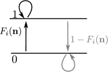
Figure 1: State transitions of a binary neuron. Each neuron is updated at random time points, intervals are i.i.d. exponential with mean duration $\tau$, so the rate of updates per neuron $i$ is $\tau^{-1}$. The probability of neuron $i$ to end in the up-state ($1$) is determined by the gain function $F_{i}(\mathbf{n})$ which potentially depends on the states $\mathbf{n}$ of all neurons in the network. The up-transitions are indicated by black arrows. The probability for the down state ($0$) is given by the complementary probability $1-F_{i}(\mathbf{n})$, indicated by gray arrows.

The neuron model shows stochastic transitions (at random points in time) between the two states $0$ and $1$ controlled by transition probabilities, as illustrated in Figure 1. Using asynchronous update [52], in each infinitesimal interval $[t,t+\delta t)$ each neuron in the network has the probability $\frac{1}{\tau}\delta t$ to be chosen for update [26], where $\tau$ is the time constant of the neuronal dynamics. An equivalent implementation draws the time points of update independently for all neurons. For a particular neuron, the sequence of update points has exponentially distributed intervals with mean duration $\tau$, i.e. update times form a Poisson process with rate $\tau^{-1}$. We employ the latter implementation in the globally time-driven [21] spiking simulator NEST [15], and use a discrete time resolution $\delta t=0.1\,\mathrm{ms}$ for the intervals. The stochastic update constitutes a source of noise in the system. Given the $i$-th neuron is selected for update, the probability to end in the up-state ($n_{i}=1$) is determined by the gain function $F_{i}(\mathbf{n})$ which possibly depends on the activity $\mathbf{n}$ of all other neurons. The probability to end in the down state ($n_{i}=0$) is $1-F_{i}(\mathbf{n})$. This model has been considered earlier [25, 18, 9], and here we follow the notation introduced in the latter work.

The stochastic system is completely characterized by the joint probability distribution $p(\mathbf{n})$ in all $N$ binary variables $\mathbf{n}$. Knowing the joint probability distribution, arbitrary moments can be calculated, among them pairwise correlations. Here we are only concerned with the stationary state of the network. A stationary solution of $p(\mathbf{n})$ implies that for each state a balance condition holds, so that the incoming and outgoing probability fluxes sum up to zero. The occupation probability of the state is then constant. We denote as $\mathbf{n}_{i+}=(n_{1},\ldots,n_{i-1},1,n_{i+1},\ldots,n_{N})$ the state, where the $i$-th neuron is active ($n_{i}=1$), and $\mathbf{n}_{i-}$ where neuron $i$ is inactive ($n_{i}=0$). Since in each infinitesimal time interval at most one neuron can change state, for each given state $\mathbf{n}$ there are $N$ possible transitions (each corresponding to one of the $N$ neurons changing state). The sum of the probability fluxes into the state and out of the state must compensate to zero [31], so

$$0=\tau\frac{\partial p(\mathbf{n})}{\partial t} = \sum_{i=1}^{N}\underbrace{(2n_{i}-1)}_{\text{direction of flux}}\left(\underbrace{p(\mathbf{n}_{i-})F_{i}(\mathbf{n}_{i-})}_{\text{neuron }i\text{ transition up}}-\underbrace{p(\mathbf{n}_{i+})(1-F_{i}(\mathbf{n}_{i+}))}_{\text{neuron }i\text{ transition down}}\right)\quad\forall\quad\mathbf{n}\in\{0,1\}^{N}.$$ (1)

From this equation we derive expressions for the first $\langle n_{k}\rangle$ and second moments $\langle n_{k}n_{l}\rangle$ by multiplying with $n_{k}n_{l}$ and summing over all possible states $\mathbf{n}\in\{0,1\}^{N}$, which leads to

$$0 = \sum_{\mathbf{n}\in\{0,1\}^{N}}\sum_{i=1}^{N}n_{k}n_{l}(2n_{i}-1)\underbrace{\left(p(\mathbf{n}_{i-})F_{i}(\mathbf{n}_{i-})-p(\mathbf{n}_{i+})(1-F_{i}(\mathbf{n}_{i+}))\right)}_{\equiv G_{i}(\mathbf{n}\backslash n_{i})}.$$

Note that the term denoted $G_{i}(\mathbf{n}\backslash n_{i})$ does not depend on the state of neuron $i$. We use the notation $\mathbf{n}\backslash n_{i}$ for the state of the network excluding neuron $i$, i.e. $\mathbf{n}\backslash n_{i}=(n_{1},\ldots,n_{i-1},n_{i+1},\ldots,n_{N})$. Separating the terms in the sum over $i$ into those with $i\neq k,l$ and the two terms with $i=k$ and $i=l$, we obtain

$$0 = \sum_{\mathbf{n}}\;\sum_{i=1,i\neq k,l}^{N}n_{k}n_{l}(2n_{i}-1)\,G_{i}(\mathbf{n}\backslash n_{i})+n_{k}n_{l}(2n_{k}-1)\,G_{k}(\mathbf{n}\backslash n_{k})+n_{k}n_{l}(2n_{l}-1)\,G_{l}(\mathbf{n}\backslash n_{l})$$

$$= \sum_{i=1,i\neq k,l}^{N}\;\sum_{\mathbf{n}\backslash n_{i}}n_{k}n_{l}(G_{i}(\mathbf{n}\backslash n_{i})-G_{i}(\mathbf{n}\backslash n_{i}))+\sum_{\mathbf{n}}n_{k}n_{l}\,G_{k}(\mathbf{n}\backslash n_{k})+\sum_{\mathbf{n}}n_{k}n_{l}\,G_{l}(\mathbf{n}\backslash n_{l})$$

where we obtained the first term by explicitly summing over state $n_{i}\in\{0,1\}$ (i.e. using $\sum_{\mathbf{n}\in\{0,1\}^{N}}=\sum_{\mathbf{n}\backslash n_{i}\in\{0,1\}^{N-1}}\sum_{n_{i}=0}^{1}$ and evaluating the sum $\sum_{n_{1}=0}^{1}$). This first sum obviously vanishes. The remaining terms are of identical form with the roles of $k$ and $l$ interchanged. We hence only consider the first of them and obtain the other by symmetry. The first term simplifies to

$$\sum_{\mathbf{n}}n_{k}n_{l}\,G_{k}(\mathbf{n}\backslash n_{k})\stackrel{{\scriptstyle n_{k}=1}}{{=}}\sum_{\mathbf{n}\backslash n_{k}}n_{l}\,G_{k}(\mathbf{n}\backslash n_{k})$$

$$\stackrel{{\scriptstyle\text{def. }G_{k}}}{{=}} \begin{cases}\sum_{\mathbf{n}\backslash n_{k}}p(\mathbf{n}_{k-})\,F_{k}(\mathbf{n}_{k-})+p(\mathbf{n}_{k+})\,F_{k}(n_{k+})-p(\mathbf{n}_{k+})&\quad\text{for }k=l\\ \sum_{\mathbf{n}\backslash n_{k}}p(\mathbf{n}_{k-})\,n_{l}\,F_{k}(\mathbf{n}_{k-})+p(\mathbf{n}_{k+})\,n_{l}\,F_{k}(n_{k+})-n_{l}\,p(\mathbf{n}_{k+})&\quad\text{for }k\neq l\end{cases}$$

$$= \begin{cases}\langle F_{k}(\mathbf{n})\rangle-\langle n_{k}\rangle&\text{for }k=l\\ \langle F_{k}(\mathbf{n})\,n_{l}\rangle-\langle n_{k}n_{l}\rangle&\text{for }k\neq l\end{cases},$$

where we denote as $\langle f(\mathbf{n})\rangle=\sum_{\mathbf{n}\in\{0,1\}^{N}}p(\mathbf{n})f(\mathbf{n})$ the average of a function $f(\mathbf{n})$ with respect to the distribution $p(\mathbf{n})$. Taken together with the mirror term $k\leftrightarrow l$, we arrive at two conditions, one for the first ($k=l$, $\langle n_{k}^{2}\rangle=\langle n_{k}\rangle$) and one for the second ($k\neq l$) moment

$$2\langle n_{k}n_{l}\rangle = \begin{cases}2\langle F_{k}(\mathbf{n})\rangle&\text{for }k=l\\ \langle F_{k}(\mathbf{n})\,n_{l}\rangle+\langle F_{l}(\mathbf{n})\,n_{k}\rangle&\text{for }k\neq l\end{cases}.$$ (2)

Considering the covariance $c_{kl}=\langle\delta n_{k}\delta n_{l}\rangle$ with centralized variables $\delta n_{k}=n_{k}-\langle n_{k}\rangle$, for $k\neq l$ one arrives at

$$2c_{kl} = \langle F_{k}(\mathbf{n})\,\delta n_{l}\rangle+\langle F_{l}(\mathbf{n})\,\delta n_{k}\rangle.$$ (3)

This equation is identical to eq. 3.9 in [18], to eqs. 3.12 and 3.13 in [9], and to eqs. (19)-(22) in [49, Supplementary material].

Mean-field solution

Starting from (1) for the general case $\frac{\partial p(\mathbf{n},t)}{\partial t}\neq 0$, a similar calculation as the one resulting in (2) for $k=l$ leads to

$$\tau\frac{\partial}{\partial t}\langle n_{k}\rangle = \langle F_{k}(\mathbf{n})\rangle-\langle n_{k}\rangle,$$

where we used $\langle n_{k}^{2}\rangle=\langle n_{k}\rangle$, valid for binary variables. As in [49] we now assume a particular form for the gain function and for the coupling between neurons by specifying

$$F_{k}(\mathbf{n}) = H\left(h_{k}-\theta\right)$$

$$h_{k} = \sum_{l=1}^{N}J_{kl}n_{l}$$

$$H(x) = \begin{cases}1&\text{if }x\geq 0\\ 0&\text{if }x<0\end{cases},$$

where $J_{kl}$ is the incoming synaptic weight from neuron $l$ to neuron $k$, $H$ is the Heaviside function, and $\theta$ is the threshold of the activation function. For positive $\theta$ the neuron gets activated only if sufficient excitatory input is present and for negative $\theta$ the neuron is intrinsically active even in the absence of excitatory input. We denote by $h_{k}$ the summed synaptic input to the neuron, sometimes also called the “field”. Because $n_{k}^{2}=n_{k}$, the variance $a_{k}$ of a binary variable is $a_{k}\equiv\langle n_{k}^{2}\rangle-\langle n_{k}\rangle^{2}=(1-\langle n_{k}\rangle)\langle n_{k}\rangle.$ We now aim to solve (2) for the case $k=l$, i.e. the equation $\langle n_{k}\rangle=\langle F_{k}\rangle$. In general, the right hand side depends on the fluctuations of all neurons projecting to neuron $k$. An exact solution is therefore complicated. However, for sufficiently irregular activity in the network we assume the neurons to be approximately independent. Further assume that in a network of homogeneous populations $\alpha$ (same parameters $\tau$, $\theta$ and same statistics of the incoming connections for all neurons, i.e. same number $K_{\alpha\beta}$ and strength $J_{\alpha\beta}$ of incoming connections from neurons in a given population $\beta$) the mean activity of an individual neuron can be represented by the population mean $m_{\alpha}=\langle\frac{1}{N_{\alpha}}\sum_{i\in\alpha}n_{i}\rangle$. The mean input to a neuron in population $\alpha$ then is

$$\langle h_{\alpha}\rangle = \sum_{\beta}K_{\alpha\beta}J_{\alpha\beta}m_{\beta}\equiv\mu_{\alpha}.$$ (4)

We assumed in the last step identical synaptic amplitudes $J_{\alpha\beta}$ for a synapse from a neuron in population $\beta$ to a neuron in population $\alpha$. So the input to each neuron has the same mean $\langle h_{\alpha}\rangle$. As a first approximation, if the mean activity in the network is not saturated, i.e. neither $0$ nor $1$, mapping this activity back by the inverse gain function to the input, $h_{\alpha}$ must be close to the threshold value, so

$$\langle h_{\alpha}\rangle \simeq \theta.$$ (5)

This relation may be solved for $m_{E}$ and $m_{I}$ to obtain a coarse estimate of the activity in the network [62, 63]. In mean-field approximation we assume that the fluctuations of the fields of individual neurons $h_{\alpha}$ around their mean are mutually independent, so that the fluctuations $\delta h_{\alpha}=h_{\alpha}-\langle h_{\alpha}\rangle$ of $h_{\alpha}$ are, in turn, caused by a sum of independent random variables and hence the variances add up to the variance $\sigma_{\alpha}^{2}$ of the field

$$\langle\delta h_{\alpha}^{2}\rangle = \sum_{\beta}K_{\alpha\beta}J_{\alpha\beta}^{2}m_{\beta}(1-m_{\beta})\equiv\sigma_{\alpha}^{2}.$$ (6)

As $h_{\alpha}$ is a sum of typically thousands of synaptic inputs, it approaches a Gaussian distribution $h_{\alpha}\sim\mathcal{N}(\mu_{\alpha},\sigma_{\alpha}^{2})$ with mean $\mu_{\alpha}$ and variance $\sigma_{\alpha}^{2}$. In this approximation the mean activity in the network is the solution of

$$\tau\frac{\partial}{\partial t}m_{\alpha}+m_{\alpha} = \langle F_{\alpha}(m_{E},m_{I},m_{x})\rangle\quad\forall\;\alpha\in\{E,I\}$$ (7)

$$\simeq \int_{-\infty}^{\infty}H(x-\theta)\>\mathcal{N}(\mu_{\alpha},\sigma_{\alpha}^{2},x)\,dx$$

$$= \int_{\theta}^{\infty}\mathcal{N}(\mu_{\alpha},\sigma_{\alpha}^{2},x)\,dx$$

$$= \frac{1}{2}\mathrm{erfc}\left(\frac{\theta-\mu_{\alpha}}{\sqrt{2}\sigma_{\alpha}}\right).$$

This equation needs to be self-consistently solved with $\frac{\partial m_{\alpha}}{\partial t}=0$ by numerical or graphical methods in order to obtain the stationary activity, because $\mu_{\alpha}(m_{E},m_{I},m_{x})$ and $\sigma_{\alpha}(m_{E},m_{I},m_{x})$ depend on $m_{\alpha}\forall\alpha\in\{E,I,X\}$ themselves. We here employ the algorithm $\mathrm{hybrd}$ and $\mathrm{hybrj}$ from the MINPACK package, implemented in scipy (version 0.9.0) [30] as the function $\mathrm{scipy.optimize.fsolve}$.

Linearized equation for correlations and susceptibility

In general, the term $\langle F_{k}(\mathbf{n})\,\delta n_{l}\rangle$ in (3) couples moments of arbitrary order, resulting in a moment hierarchy [9]. Here we only determine an approximate solution. Since the single synaptic amplitudes $J_{ki}$ are small, we linearize the effect of a single synaptic input. We apply the linearization to the two terms of the form $\langle F_{k}(\mathbf{n})\,\delta n_{l}\rangle$ on the right hand side of (3). In the recurrent network, the activity of each neuron in the vector $\mathbf{n}$ may be correlated to the activity of any other neuron $n_{i}$. Therefore, the input $h_{k}$ sensed by neuron $k$ not only depends on $n_{l}$ directly, but also indirectly through the correlations of $n_{l}$ with any of the other neurons $n_{i}$ that project to neuron $k$. We need to take this dependence into account in the linearization. Considering the effect of one particular input $n_{i}$ explicitly one gets

$$\langle F_{k}(\mathbf{n})\delta n_{l}\rangle = \langle H(h_{k}-\theta)\,\delta n_{l}\rangle$$

$$= \langle H(h_{k\backslash n_{i}}+J_{ki}-\theta)\,n_{i}\delta n_{l}+H(h_{k\backslash n_{i}}-\theta)\,(1-n_{i})\,\delta n_{l}\rangle$$

$$= \langle(H(h_{k\backslash n_{i}}+J_{ki}-\theta)-H(h_{k\backslash n_{i}}-\theta))\,n_{i}\delta n_{l}\rangle+\langle H(h_{k\backslash n_{i}}-\theta)\,\delta n_{l}\rangle.$$

The first term $\langle(H(h_{k\backslash n_{i}}+J_{ki}-\theta)-H(h_{k\backslash n_{i}}-\theta))\,n_{i}\delta n_{l}\rangle$ already contains two factors $n_{i}$ and $\delta n_{l}$, so it takes into account second order moments. Performing the expansion for the next input would yield terms corresponding to correlations of higher order, which are neglected here. This amounts to the assumption that the remaining fluctuations in $h_{k\backslash n_{i}}$ are independent of $n_{i}$ and $n_{l}$, and we again approximate them by a Gaussian random variable $x\sim\mathcal{N}(\mu_{k},\sigma_{k})$ with mean $\mu_{k}=\langle h_{k}\rangle$ and variance $\sigma_{k}^{2}=\langle\delta h_{k}^{2}\rangle$, so $\langle(H(x+J_{ki}-\theta)-H(x-\theta))\rangle_{x}\langle n_{i}\delta n_{l}\rangle_{\mathbf{n}}\simeq S(\mu_{k},\sigma_{k})\,J_{ki}\,\langle n_{i}\delta n_{l}\rangle_{\mathbf{n}}+O(J_{ki}^{2}).$ Here we used the smallness of the synaptic weight $J_{ki}$ and replaced the difference by the derivative $S(\mu_{k},\sigma_{k})=\left.\frac{\partial\langle H(x+J)\rangle_{x\sim\mathcal{N}(\mu_{k},\sigma_{k})}}{\partial J}\right|_{J=0}$, which has the form of a susceptibility. Using the explicit expression for the Gaussian integral (7), the susceptibility is exactly

$$S(\mu_{k},\sigma_{k}) = \frac{1}{\sqrt{2\pi}\sigma_{k}}e^{-\frac{(\mu_{k}-\theta)^{2}}{2\sigma_{k}^{2}}}.$$ (8)

The same expansion holds for the remaining inputs to cell $k$. With $\langle n_{i}\delta n_{l}\rangle=\begin{cases}a_{i}&\text{for }i=l\\ c_{il}&\text{for }i\neq l\end{cases}$, the equation for the pairwise correlations (3) in linear approximation takes the form

$$2c_{kl} = S(\mu_{k},\sigma_{k})\,\left(\sum_{j}J_{kj}c_{jl}+J_{kl}a_{l}\right)+S(\mu_{l},\sigma_{l})\,\left(\sum_{j}J_{lj}c_{jk}+J_{lk}a_{k}\right),$$ (9)

corresponding to eq. (6.8) in [18] and eqs. (31)-(33) in [49, Supplementary material]. Note, however, that the linearization used in [18] relies on the smoothness of the gain function due to additional local noise, whereas here and in [49, Supplementary material] a Heaviside gain function is used and only the existence of noise generated by the network itself justifies the linearization. If the input to each neuron is homogeneous, i.e. $\mu_{k}=\mu_{\alpha}$ and $\sigma_{k}=\sigma_{\alpha}$ for all neurons $k$ in population $\alpha$, a structurally similar equation connects the correlations $c_{\alpha\beta}=\frac{1}{N_{\alpha}N_{\beta}}\sum_{k\in\alpha,l\in\beta,k\neq l}\,c_{kl}$ averaged over disjoint pairs of neurons belonging to two (possibly identical) populations $\alpha$,$\beta$ with the population averaged variances $a_{\alpha}=\frac{1}{N_{\alpha}}\sum_{k\in\alpha}a_{k}$

$$2c_{\alpha\beta} = \sum_{\gamma\in\{E,I,X\}}\left(w_{\alpha\gamma}c_{\gamma\beta}+w_{\beta\gamma}c_{\gamma\alpha}\right)+w_{\alpha\beta}\frac{a_{\beta}}{N_{\beta}}+w_{\beta\alpha}\frac{a_{\alpha}}{N_{\alpha}}$$ (10)

$$\text{with }w_{\alpha\beta} = S(\mu_{\alpha},\sigma_{\alpha})\,J_{\alpha\beta}\,K_{\alpha\beta}.$$

In deriving the last expression, we replaced variances of individual neurons and correlations between individual pairs by their respective population averages and counted the number of connections. This equation corresponds to eqs. (9.14)-(9.16) in [18] (which lack, however, the external population $X$, and note the typo in the first term in line 2 of eq. (9.16), which should read $-\frac{1}{2}\bar{J}{}_{EI}C_{II}(0)$) and eqs. (36) in [49, Supplementary material]. Written in matrix form (10) takes the form (50) of the main text, where we defined

$$A = \left(\begin{array}[]{ccc}2-2w_{EE}&-2w_{EI}&0\\ -w_{IE}&2-\left(w_{EE}+w_{II}\right)&-w_{EI}\\ 0&-2w_{IE}&2-2w_{II}\end{array}\right)$$ (14)

$$B = \left(\begin{array}[]{cc}2w_{EE}&0\\ w_{IE}&w_{EI}\\ 0&2w_{II}\end{array}\right)\qquad C=\left(\begin{array}[]{cc}2w_{EX}&0\\ w_{IX}&w_{EX}\\ 0&2w_{IX}\end{array}\right)$$ (21)

$$D = \left(\begin{array}[]{cc}2-w_{EE}&-w_{EI}\\ -w_{IE}&2-w_{II}\end{array}\right)\qquad E=\left(\begin{array}[]{c}w_{EX}\\ w_{IX}\end{array}\right).$$ (26)

The explicit solution of the latter system of (50) is

$$\left(\begin{array}[]{c}c_{XE}\\ c_{XI}\end{array}\right) = \frac{1}{(2-w_{EE})(2-w_{II})-w_{EI}w_{IE}}\left(\begin{array}[]{c}(2-w_{II})w_{EX}+w_{EI}w_{IX}\\ (2-w_{EE})w_{IX}+w_{IE}w_{EX}\end{array}\right)\,\frac{a_{X}}{N_{X}}.$$ (31)

Mean-field theory including finite-size correlations

The mean-field solution presented in
“Mean-field solution” assumes that correlations among the neurons in the network are negligible. This assumption enters the expression (6) for the variance of the input to a neuron. Having determined the actual magnitude of the correlations in (50), we are now able to state a more accurate approximation in which we take these correlations into account, modifying the expression for the variance of the field $h_{\alpha}$

$$\sigma_{\alpha}^{2} = \sum_{\beta\in\{E,I,X\}}K_{\alpha\beta}J_{\alpha\beta}^{2}m_{\beta}(1-m_{\beta})+\sum_{\beta,\gamma\in\{E,I,X\}}(KJ)_{\alpha\beta}(KJ)_{\alpha\gamma}c_{\beta\gamma}$$ (32)

$$\text{with }(KJ)_{\alpha\beta} \equiv K_{\alpha\beta}J_{\alpha\beta}.$$

This correction suggests an iterative scheme: Initially we solve the mean-field equation (7) assuming $c_{\alpha\beta}=0$ (hence $\sigma_{\alpha}$ given by (6)). In each step of the iteration we then calculate the correlations by (50), compute the mean-field solution of (7) and the susceptibility $S(\mu_{\alpha},\sigma_{\alpha})$ (8), taking into account the correlations (32) determined in the previous step. These steps are iterated until the solution ($m_{\alpha},c_{\alpha\beta}\quad\forall\alpha,\beta$) converges. We use this approach to determine the correlation structure in Figure 3, where we iterated until the solution became invariant up to a residual absolute difference of $10^{-15}$. A comparison of the distribution of the total synaptic input $h_{E}$ at the end of the iteration with a Gaussian distribution with parameters $\mu_{E}$ and $\sigma_{E}$ is shown in Figure 3D.

Influence of inhomogeneity of in-degrees

In the previous sections we assumed the number of incoming connections to be the same for all neurons. Studying a random network in its original Erdös-Rényi [43] sense, the number of synaptic inputs $K_{i\beta}$ to a neuron $i\in\alpha$ from population $\beta$ is a binomially distributed random number. As a consequence, the time-averaged activity differs among neurons. Since each neuron $i\in\alpha$ samples a random subset of inputs from a given population $\beta$, we can assume that the realization of $K_{i\beta}$ is independent of the realization of the time-averaged activity of the inputs from population $\beta$. So these two contributions to the variability of the mean input $\delta\mu_{\alpha}^{2}$ add up. The number of incoming connections to a neuron in population $i\in\alpha$ follows a binomial distribution

$$K_{i\beta} \sim B(N_{\beta},p),$$

where $p$ is the connection probability and $N_{\beta}$ the size of the sending population. The mean value is as before $K_{\alpha\beta}=[\frac{1}{N_{\alpha}}\sum_{i\in\alpha}K_{i\beta}]=pN_{\beta}$, where we denote the expectation value with respect to the realization of the connectivity as $[]$. The variance of the in-degree is hence

$$\delta K_{\alpha\beta}^{2} =\left[\frac{1}{N_{\alpha}}\sum_{i\in\alpha}\left(K_{i\beta}-K_{\alpha\beta}\right)^{2}\right]=N_{\beta}p(1-p)=K_{\alpha\beta}(1-p).$$

In the following we adapt the results from [63, 49] to the present notation. The contribution of the variability of the number of synapses to the variance of the mean input is $\sum_{\beta}\,J_{\alpha\beta}^{2}\delta K_{\alpha\beta}^{2}m_{\beta}^{2}$. The contribution from the distribution of the mean activities can be expressed by the variance of the mean activity defined as

$$\delta m_{\alpha}^{2} \equiv\left[\frac{1}{N_{\alpha}}\sum_{i\in\alpha}m_{i}^{2}\right]-m_{\alpha}^{2}$$

$$\equiv q_{\alpha}-m_{\alpha}^{2}.$$

The $K_{\alpha\beta}$ independently drawn inputs hence contribute $\sum_{\beta}J_{\alpha\beta}^{2}K_{\alpha\beta}\delta m_{\beta}^{2}$, as the variances of the $K_{\alpha\beta}$ terms add up. So together we have [63, eq. 5.5 - 5.6]

$$\delta\mu_{\alpha}^{2} =\sum_{\beta}\,J_{\alpha\beta}^{2}(\delta K_{\alpha\beta}^{2}m_{\beta}^{2}+K_{\alpha\beta}\delta m_{\beta}^{2}).$$

Using $K_{\alpha\beta}=N_{\beta}p$ we obtain

$$\delta\mu_{\alpha}^{2} =\sum_{\beta}\,J_{\alpha\beta}^{2}\left(\delta K_{\alpha\beta}^{2}m_{\beta}{}^{2}+K_{\alpha\beta}\delta m_{\beta}^{2}\right)$$

$$=\sum_{\beta}\,J_{\alpha\beta}^{2}K_{\alpha\beta}\left((1-p)\,m_{\beta}^{2}+q_{\beta}-m_{\beta}^{2}\right)$$

$$=\sum_{\beta}\,J_{\alpha\beta}^{2}K_{\alpha\beta}\left(q_{\beta}-p\,m_{\beta}^{2}\right).$$ (33)

The latter expression differs from [63, eq. 5.7] only in the term $-pm_{\beta}^{2}$ that is absent in the work of van Vreeswijk and Sompolinsky, because they assumed the number of synapses to be Poisson distributed in the limit of sparse connectivity [63, Appendix, (A.6)] (also note that their $J_{kl}$ corresponds to our $\sqrt{K_{\alpha\beta}}J_{\alpha\beta}$). The expression (33) is identical to [49, Supplementary, eq. (25)].

Since the variance of a binary signal with time-averaged activity $m_{i}$ is $m_{i}(1-m_{i})$, the population-averaged variance is hence

$$a_{\alpha}=\frac{1}{N_{\alpha}}\sum_{i\in\alpha}[m_{i}(1-m_{i})] =m_{\alpha}-q_{\alpha}.$$ (34)

So the sum of $K_{\alpha\beta}$ such (uncorrelated) signals contributes to the fluctuation of the input as

$$\sigma_{\alpha}^{2}=[\delta h_{\alpha}^{2}] =\sum_{\beta}\,J_{\alpha\beta}^{2}K_{\alpha\beta}(m_{\beta}-q_{\alpha}).$$ (35)

The contribution due to the variability of the number of synapses $\delta K_{\alpha\beta}^{2}$ can be neglected in the limit of large networks [49]. The time-averaged activity of a single cell with mean input $\mu_{i}$ and variance $\sigma_{i}^{2}$ is given, as before by (7) $m_{i}=\Phi(\mu_{i},\sigma_{i})$, so the distribution of activity in the population is

$$p(m) =\int_{-\infty}^{\infty}\delta(m-\Phi(x,\sigma_{\alpha}))\,\mathcal{N}(\mu_{\alpha},\delta\mu_{\alpha}^{2},x)\,dx$$

$$=\left(\Phi^{\prime}\right)^{-1}(\Phi^{-1}(m))\,\mathcal{N}(\mu_{\alpha},\delta\mu_{\alpha}^{2},\Phi^{-1}(m)).$$ (36)

The mean activity of the whole population is

$$m_{\alpha} =\int_{-\infty}^{\infty}\mathcal{N}(\mu_{\alpha},\delta\mu_{\alpha}^{2},y)\,\Phi(y,\sigma_{\alpha}^{2})\,dy$$

$$=\int_{-\infty}^{\infty}\mathcal{N}(\mu_{\alpha},\delta\mu_{\alpha}^{2},y)\,\int_{\theta}^{\infty}\mathcal{N}(y,\sigma_{\alpha}^{2},x)\,dx\,dy$$

$$=\int_{\theta}^{\infty}\int_{-\infty}^{\infty}\mathcal{N}(\mu_{\alpha},\delta\mu_{\alpha}^{2},y)\,\mathcal{N}(y,\sigma_{\alpha}^{2},x)\,dy\,dx$$

$$=\Phi(\mu_{\alpha},\sigma_{\alpha}^{2}+\delta\mu_{\alpha}^{2}),$$ (37)

because the penultimate line is a convolution of two Gaussian distributions, so the means and variances add up. The second moment of the population activity is

$$q_{\alpha} =\int_{-\infty}^{\infty}\mathcal{N}(\mu_{\alpha},\delta\mu_{\alpha}^{2},x)\,\Phi^{2}(x,\sigma_{\alpha}^{2})\,dx.$$ (38)

These expressions are identical to [49, Supplementary, eqs. (26), (27)]. The system of equations (4), (33), (35), (37), and (38) can be solved self-consistently. We use the algorithm $\mathrm{hybrd}$ and $\mathrm{hybrj}$ of the MINPACK package, implemented in scipy (version 0.9.0) [30] as the function $\mathrm{scipy.optimize.fsolve}$. This yields the self-consistent solutions for $m_{\alpha}$ and $q_{\alpha}$ and hence the distribution of time averaged activity (36) can be obtained, shown in Figure 6F.

Results

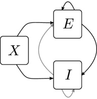
Figure 2: Recurrent local network of two populations of excitatory ($E$) and inhibitory ($I$) neurons driven by a common external population ($X$). The external population $X$ delivers stochastic activity to the local network. The local network is a recurrent Erdős-Rényi random network with homogeneous synaptic weights $J_{\alpha\beta}$ coupling neurons in population $\beta$ to neurons in population $\alpha$, for $\alpha,\beta\in\{E,I\}$ and same parameters for all neurons. There are $N=8192$ neurons in both the excitatory and the inhibitory population. The connection probability is $p=0.2$, and each neuron in population $\alpha$ receives the same number $K=pN$ of excitatory and inhibitory synapses. The size $N_{X}$ of the external population determines the amount of shared input received by each pair of cells in the local network. The neurons are modeled as binary units with a hard threshold $\theta$.

Our aim is to investigate the effect of recurrence and external input on the magnitude and structure of cross-correlations between the activities in a recurrent random network, as defined in “Networks of binary neurons”. We employ the established recurrent neuronal network model of binary neurons in the balanced regime [62]. The binary dynamics has the advantage to be more easily amendable to analytical treatment than spiking dynamics. A method to calculate the pairwise correlations exists since long [18]. The choice of binary dynamics moreover renders our results directly comparable to the recent findings on decorrelation in such networks [49]. Our model consists of three populations of neurons, one excitatory and one inhibitory population which together represent the local network, and an external population providing additional excitatory drive to the local network, as illustrated in Figure 2. The external population may either be conceived as representing input into the local circuit from remote areas or as representing sensory input. The external population contains $N_{X}$ neurons, which are pairwise uncorrelated and have a stochastic activity with mean $m_{X}$. Each neuron in population $\alpha\in\{E,I\}$ within the local network draws $K=pN$ connections randomly from the finite pool of $N_{X}$ external neurons. $N_{X}$ therefore determines the number of shared afferents received by each pair of cells from the external population with on average $K^{2}/N_{X}$ common synapses. In the extreme cases $N_{X}=K$ all neurons receive exactly the same input, whereas for large $N_{X}\rightarrow\infty$ the fraction of shared external input approaches $0$. The common fluctuating input received from the finite-sized external population hence provides a signal imposing pairwise correlations, the amount of which is controlled by the parameter $N_{X}$.

Correlations are driven by intrinsic and external fluctuations

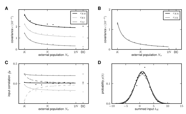
Figure 3: Correlations in a network of three populations as illustrated in Figure 2 in dependence of the size $N_{x}$ of the external population. Each neuron in population $\alpha\in\{E,I\}$ receives $pN$ randomly drawn excitatory inputs with weight $J_{\alpha E}=\frac{5}{\sqrt{N}}$, $pN$ randomly drawn inhibitory inputs of weight $J_{\alpha I}=-\frac{10}{\sqrt{N}}$ and $pN$ external inputs of weight $J_{\alpha X}=\frac{5}{\sqrt{N}}$ (homogeneous random network with fixed in-degree, connection probability $p=0.2$). A Correlations averaged over pairs of neurons within the local network (41). Dots indicate results of direct simulation over $T=30\,\mathrm{s}$ averaged over $(N/2)^{2}$ pairs of neurons. Curves show the analytical result (50). The point “DC” shows the correlation structure emerging if the drive from the external population is replaced by a constant value $KJ_{\alpha X}m_{X}$, which provides the same mean input as the original external drive. B Correlations between neurons within the local network and the external population averaged over pairs of neurons (same labeling as in A). C Correlation between the inputs to a pair of cells in the network decomposed into the contributions due to shared inputs $c_{\mathrm{shared}}$ (gray, eq. 54) and due to correlations $c_{\mathrm{corr}}$ in the presynaptic activity (light gray, eq. 55). Dashed curves and St. Andrew’s Crosses show the contribution due to external inputs, solid curves and dots show the contribution from local inputs. The sum of all components is shown by black dots and curve. Curves are theoretical results based on (50), (54), and (55), symbols are obtained from simulation. D Probability distribution of the fluctuating input $h_{E}$ to a single neuron in the excitatory population. Dots show the histogram obtained from simulation binned over the interval $[\min(h_{E}),\max(h_{E})]$ with a bin size of $-2J_{\alpha I}$. The gray curve is the prediction of a Gaussian distribution obtained from mean-field theory neglecting correlations, with mean and variance given by (4) and (6), respectively. The black curve takes correlations in the afferent signals into account and has a variance given by (32). Other parameters: simulation resolution $\Delta t=0.1\,\mathrm{ms}$, synaptic delay $d=\Delta t$, activity measurement in intervals of $1\,\mathrm{ms}$. Threshold of the neurons $\theta=1$, time constant of inter-update intervals $\tau=10\,\mathrm{ms}$. The average activity in the network is $m_{E}\simeq m_{I}\simeq m_{X}=0.5$.

To explain the correlation structure observed in a network with external inputs (Figure 2), we extend the existing theory of pairwise correlations [18] to include the effect of externally imposed correlations. The global behavior of the network can be studied with the help of the mean-field equation (7) for the population-averaged mean activity $m_{\alpha}=N_{\alpha}^{-1}\sum_{i\in\alpha}\langle n_{i}\rangle$

$$m_{\alpha} = \frac{1}{2}\mathrm{erfc}\left(\frac{\theta-\mu_{\alpha}}{\sqrt{2}\sigma_{\alpha}}\right)=\Phi(\mu_{\alpha},\sigma_{\alpha}),$$ (39)

where the fluctuations of the input $h_{\alpha}$ to a neuron in population $\alpha$ are to good approximation Gaussian with the moments

$$\mu_{\alpha}=\langle h_{\alpha}\rangle = \sum_{\beta}K_{\alpha\beta}J_{\alpha\beta}m_{\beta}$$ (40)

$$\sigma_{\alpha}^{2}=\langle\delta h_{\alpha}^{2}\rangle = \sum_{\beta}K_{\alpha\beta}J_{\alpha\beta}^{2}m_{\beta}(1-m_{\beta}).$$

To determine the average activities in the network, the mean-field equation (39) needs to be solved self-consistently, as the right-hand side depends on the mean activities $m_{\alpha}$ through (40), as explained in “Mean-field theory including finite-size correlations”. Here $K_{\alpha\beta}$ denotes the number of connections from population $\beta$ to $\alpha$, and $J_{\alpha\beta}$ their average synaptic amplitude. Once the mean activity in the network has been found, we can determine the structure of correlations. For simplicity we focus on the zero time lag correlation, $c_{ij}=\langle\delta n_{i}(t)\delta n_{j}(t)\rangle_{t}$, where $\delta n_{i}(t)=n_{i}(t)-\langle n_{i}\rangle_{t}$ is the deflection of neuron $i$’s activity from baseline and $a_{i}=\langle\delta n_{i}^{2}(t)\rangle_{t}=\langle n_{i}\rangle_{t}(1-\langle n_{i}\rangle_{t})$ is the variance of neuron $i$’s activity. Starting from the master equation for the network of binary neurons, in “Methods” for completeness and consistency in notation we re-derive the self-consistent equation that connects the cross covariances $c_{\alpha\beta}$ averaged over pairs of neurons from population $\alpha$ and $\beta$ and the variances $a_{\alpha}$ averaged over neurons from population $\alpha$

$$c_{\alpha\beta} = \frac{1}{N_{\alpha}N_{\beta}}\sum_{k\in\alpha,l\in\beta,k\neq l}\,c_{kl}$$ (41)

$$a_{\alpha} = \frac{1}{N_{\alpha}}\sum_{k\in\alpha}a_{k}.$$

The obtained inhomogeneous system of linear equations (50) reads [18]

$$2c_{\alpha\beta} = \frac{1}{N_{\beta}}w_{\alpha\beta}a_{\beta}+\sum_{\gamma\in\{E,I,x\}}w_{\alpha\gamma}c_{\gamma\beta}+\text{transpose}(\alpha\leftrightarrow\beta).$$ (42)

Here $w_{\alpha\beta}=S(\mu_{\alpha},\sigma_{\alpha})\,K_{\alpha\beta}\,J_{\alpha\beta}$ measures the effective linearized coupling strength from population $\beta$ to population $\alpha$. It depends on the number of connections $K_{\alpha\beta}$ from population $\beta$ to $\alpha$, their average synaptic amplitude $J_{\alpha\beta}$ and the susceptibility $S_{\alpha}$ of neurons in population $\alpha$. The susceptibility $S(\mu_{\alpha},\sigma_{\alpha})$ given by (8) quantifies the influence a fluctuation in the input to a neuron in population $\alpha$ has on the output. It depends on the working point $(\mu_{\alpha},\sigma_{\alpha})$ of the neurons in population $\alpha$. The autocorrelations $a_{E}$, $a_{I}$ and $a_{X}$ are the inhomogeneity in the system of equations, so they drive the correlations, as pointed out earlier [18]. This is in line with the linear theories [58, 23] for leaky integrate-and-fire model neurons, where cross-correlations are proportional to the auto-correlations. The system of equations (42) is identical to [18, eqs. (9.14)-(9.16)]. Note that this description holds for finite-sized networks. With the symmetry $c_{EI}=c_{IE}$, (42) can be written in matrix form as

$$A\left(\begin{array}[]{c}c_{EE}\\ c_{EI}\\ c_{II}\end{array}\right) = B\,\left(\begin{array}[]{c}\frac{a_{E}}{N_{E}}\\ \frac{a_{I}}{N_{I}}\end{array}\right)+C\,\left(\begin{array}[]{c}c_{EX}\\ c_{IX}\end{array}\right)$$ (50)

$$D\left(\begin{array}[]{c}c_{EX}\\ c_{IX}\end{array}\right) = E\,\frac{a_{X}}{N_{X}}.$$ (53)

The explicit forms of the matrices $A,\ldots,E$ are given in (26). This system of linear equations can be solved by elementary methods. From the structure of the equations it follows, that the correlations between the external input and the activity in the network, $c_{EX}$ and $c_{IX}$, are independent of the other correlations in the network. They are solely determined by the solution of the system of equations in the second line of (50), driven by the fluctuations of the external drive $a_{X}/N_{X}$. The correlations among the neurons within the network are given by the solution of the first system in (50). They are hence driven by two terms, the fluctuations of the neurons within the network proportional to $a_{E}/N_{E}$ and $a_{I}/N_{I}$ and the correlations between the external population and the neurons in the network, $c_{EX}$ and $c_{IX}$.

The second line of (50) shows that all correlations depend on the size $N_{X}$ of the external population. Since the number $K=pN$ of randomly drawn afferents per neuron from this population is constant, the mean number of shared inputs to a pair of neurons is $K^{2}/N_{X}$. In the extreme case $N_{X}=K$ on the left of Figure 3 all neurons receive exactly identical input. If the recurrent connectivity would be absent, we would hence have perfectly correlated activity within the local network, the covariance between two neurons would be equal to their variance $a_{\alpha}=m_{\alpha}(1-m_{\alpha})$, in this particular network $a_{\alpha}\simeq 0.25$. Figure 3A shows that the covariance in the recurrent network is much smaller; on the order of $10^{-4}$. The reason is the recently reported mechanism of decorrelation [49], explained by the negative feedback in inhibition-dominated networks [58]. Increasing the size of the external population decreases the amount of shared input, as seen in Figure 3C. In the limit where the external drive is replaced by a constant value (shown as point “DC”), the external drive does consequently not contribute to correlations in the network. Figure 3A shows that the relative position of the three curves does not change with $N_{X}$. The overall offset, however, changes. This can be understood by inspecting the analytical result (50): The solution of this system of linear equations is a superposition of two contributions. One is due to the externally imposed fluctuations, proportional to $a_{X}/N_{X}$, the other is due to fluctuations generated within the local network, proportional to $a_{E}/N_{E}$ and $a_{I}/N_{I}$. Varying the size of the external population only changes the external contribution, causing the variation in the offset, while the internal contribution, causing the splitting between the three curves, remains constant. In the extreme case $a_{X}=0$ (DC input), we still observe a similar structure. The slightly larger splitting is due to the reduced variance $\sigma_{\alpha}^{2}$ in the single neuron input, which consequently increases the susceptibility $S_{\alpha}$ (8).

Figure 3D shows the probability distribution of the input $h_{\alpha}$ to a neuron in population $\alpha=E$. The histogram is well approximated by a Gaussian. The first two moments of this Gaussian are $\mu_{\alpha}$ and $\sigma_{\alpha}^{2}$ given by (40), if correlations among the afferents are neglected. This approximation deviates from the result of direct simulation. Taking the correlations among the afferents into account affects the variance in the input according to (32). The latter approximation is a better estimate of the input statistics, as shown in Figure 3D. This improved estimate can be accounted for in the solution of the mean-field equation (39), which in turn affects the correlations via the susceptibility $S_{\alpha}$. Iterating this procedure until convergence, as explained in “Mean-field theory including finite-size correlations”, yields the semi-analytical results presented in Figure 3.

Cancellation of input correlations

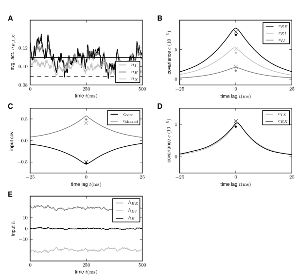
Figure 4: Activity in a network of $3N=3\times 8192$ binary neurons with synaptic amplitudes $J_{\alpha E}=J_{\alpha X}=5/\sqrt{N}$, $J_{\alpha I}=-10/\sqrt{N}$ depending exclusively on the type of the sending neuron ($E$ or $I$). Each neuron receives $K=pN$ randomly drawn inputs (fixed in-degree, $p=0.2$). A Population averaged activity (black $E$, gray $I$, light gray $X$). Analytical prediction (5) for the mean activities $m_{E}=m_{I}$ (dashed horizontal line) and numerical solution of mean field equation (7) (solid horizontal line). B Cross covariance between excitatory neurons (black), between inhibitory neurons (gray), and between excitatory and inhibitory neurons (light gray). Theoretical results (50) shown as dots. St. Andrew’s Crosses indicate the theoretical prediction of leading order in $N^{-1}$ (130). C Correlation between the input currents to a pair of excitatory neurons. The black curve is the contribution due to pairwise correlations $c_{\mathrm{corr}}$, the gray curve is the contribution of shared input $c_{\mathrm{shared}}$. The symbols show the theoretical expectation (54) and (55) based on (130) (crosses) and based on (50) (dots). D Similar to B, but showing the correlations between external neurons and neurons in the excitatory and inhibitory population. Note that both theories yield $c_{EX}=c_{IX}$, so for each theory ((130) crosses, (50) dots) only the symbol for $c_{EX}$ is visible. E Contributions $h_{EE}$ (gray) due to excitatory synapses and $h_{EI}$ (light gray) due to inhibitory synapses to the input $h_{E}$ averaged over all excitatory neurons. Duration of simulation $T=100\mathrm{\,s}$, mean activity $m_{X}=0.1$, $m_{E}\simeq m_{I}\simeq 0.11$, other parameters as in Figure 3.

We would like to understand how the structure of correlations relates to the earlier report of fast tracking [62, 63]. Small correlations observed in balanced recurrent networks were explained by the property of recurrent networks to track their input on a fast time-scale [49, their eq. (2)]. Figure 4A shows the population activities in a network of three populations for fixed numbers of neurons $N_{x}=N_{E}=N_{I}=N$ and symmetric connectivity as in Figure 3. The deflections of the excitatory and the inhibitory population partly resemble those of the external drive to the network, but partly the fluctuations seem to be independent. Our theoretical result for the correlation structure explains this result (50): the fluctuations in the network are not only driven by external input (proportional to $a_{X}$), but are also driven by the fluctuations generated within the local populations (proportional to $a_{E}$ and $a_{I}$). The idea of fast tracking of the external signal was derived from the observation that the fluctuations in the population-averaged input $h_{\alpha}=\frac{1}{N_{\alpha}}\sum_{i\in\alpha}h_{i}$ are suppressed [49]. This suppression can be observed by decomposing the input $h_{\alpha}$ to the population $\alpha$ into contributions from excitatory (including external neurons) and from inhibitory cells, $h_{\alpha E}=(KJ)_{\alpha E}n_{E}+(KJ)_{\alpha X}n_{X}$ and $h_{\alpha I}=(KJ)_{\alpha I}n_{I}$, respectively, where we used the short hand $(KJ)_{\alpha\beta}=K_{\alpha\beta}J_{\alpha\beta}$. As shown in Figure 4E, the contributions of excitation and inhibition cancel each other so that the total input fluctuates close to the threshold (here $\theta=1$) of the neurons: the network is in the balanced state [62]. Moreover, this cancellation not only holds for the mean value, but also for fast fluctuations, which are consequently reduced in the sum $h_{\alpha}$ compared to the individual components $h_{\alpha E}$ and $h_{\alpha I}$ (Figure 4E). We will now show that this suppression of fluctuations directly implies a relation for the correlation $\langle\delta h_{i}\delta h_{j}\rangle$ between the inputs to a pair $(i,j)$ of individual neurons. There are two distinct contributions to this correlation $\langle\delta h_{i}\delta h_{j}\rangle=c_{\mathrm{shared},\alpha}+c_{\mathrm{corr},\alpha}$, one due to common inputs shared by the pair of neurons (both neurons $i,j$ assumed to belong to population $\alpha$)

$$c_{\mathrm{shared},\alpha} = \sum_{\beta\in\{E,I,X\}}(KJ)_{\alpha\beta}^{2}\frac{a_{\beta}}{N_{\beta}}$$ (54)

and one due to the correlations between afferents

$$c_{\mathrm{corr},\alpha} = \sum_{\beta,\gamma\in\{E,I,X\}}(KJ)_{\alpha\beta}(KJ)_{\alpha\gamma}c_{\beta\gamma}.$$ (55)

Figure 4C shows these two contributions to be of opposite sign but approximately same magnitude. Figure 3C shows a further decomposition of the input correlation into contributions due to the external sources and due to connections from within the local network. The sum of all components is much smaller than each individual component. This cancellation is equivalent to small fluctuations in the population-averaged input $\langle\delta h_{\alpha}^{2}\rangle\simeq 0$, because

$$0\simeq\langle\delta h_{\alpha}^{2}\rangle=\left\langle\left(\sum_{\beta\in\{E,I,X\}}(KJ)_{\alpha\beta}\delta n_{\beta}\right)^{2}\right\rangle = \sum_{\beta,\gamma\in\{E,I,X\}}(KJ)_{\alpha\beta}(KJ)_{\alpha\gamma}\langle\delta n_{\beta}\delta n_{\gamma}\rangle$$

$$= \sum_{\beta\in\{E,I,X\}}(KJ)_{\alpha\beta}^{2}\,\frac{a_{\beta}}{N_{\beta}}+\sum_{\beta,\gamma\in\{E,I,X\}}(KJ)_{\alpha\beta}(KJ)_{\alpha\gamma}\,c_{\beta\gamma}$$

$$= c_{\mathrm{shared,\alpha}}+c_{\mathrm{corr},\alpha},$$

where in the second step we used the general relation between the covariance $\langle\delta n_{\beta}\delta n_{\gamma}\rangle$ among two population averaged signals $n_{\beta}$ and $n_{\gamma}$, the population-averaged variance $a_{\beta}$, and the pairwise averaged covariances $c_{\beta\gamma}$, which reads [58, cf. eq. (1)]

$$\langle\delta n_{\beta}\delta n_{\gamma}\rangle = \left\langle\frac{1}{N_{\beta}N_{\gamma}}\sum_{i\in\beta,j\in\gamma}\delta n_{i}\delta n_{j}\right\rangle$$

$$= \delta_{\beta\gamma}\frac{1}{N_{\beta}^{2}}\sum_{i\in\beta}\langle\delta n_{i}^{2}\rangle+\frac{1}{N_{\beta}N_{\gamma}}\sum_{i\in\beta,j\in\gamma,i\neq j}\langle\delta n_{i}\delta n_{j}\rangle$$

$$= \delta_{\beta\gamma}\frac{1}{N_{\beta}}a_{\beta}+c_{\beta\gamma}.$$

Figure 5: Suppression of correlations by purely inhibitory feedback in absence of external fluctuations. Activity in a network of $N=1000$ binary inhibitory neurons with synaptic amplitudes $J=-\frac{8}{\sqrt{N}}$. Each neuron receives $K=pN$ randomly drawn inputs (fixed in-degree) with $p=0.1$. A Population averaged activity. Numerical solution of mean field equation (7) (solid horizontal line). B Cross covariance between inhibitory neurons. Theoretical result (67) shown as dot. St. Andrew’s Cross indicates the leading order term $c=-\frac{a}{N}$. C Correlation between the input currents to a pair of excitatory neurons. The black curve is the contribution due to pairwise correlations $c_{\mathrm{corr}}$, the gray curve is the contribution of shared input $c_{\mathrm{shared}}$. The dot symbols show the theoretical expectations (68) based on the leading order (crosses) and based on the full solution (67) (dot). Threshold of neurons $\theta=\frac{1}{10}pNJ+\frac{J}{2}$.

This suppression of fluctuations in the population-averaged input is a consequence of the overall negative feedback in these networks: a fluctuation $\delta h_{\alpha}$ of the population averaged input $h_{\alpha}$ causes a response in network activity which is coupled back with a negative sign, counteracting its own cause and hence suppressing the fluctuation $\delta h_{\alpha}$. Expression (Cancellation of input correlations) is an algebraic identity showing that hence also correlations between the total inputs to a pair of cells must be suppressed. Qualitatively this property can be understood by inspecting the mean-field equation (7) for the population-averaged activities, where we linearized the gain function $\Phi$ around the stationary mean-field solution to obtain

$$\tau\frac{d}{dt}\left(\begin{array}[]{c}\delta n_{E}\\ \delta n_{I}\end{array}\right)-\left(\begin{array}[]{c}\delta n_{E}\\ \delta n_{I}\end{array}\right) = \left(\begin{array}[]{cc}w_{EE}&w_{EI}\\ w_{IE}&w_{II}\end{array}\right)\left(\begin{array}[]{c}\delta n_{E}\\ \delta n_{I}\end{array}\right)+\text{noise}$$ (66)

$$\text{with }w_{\alpha\beta} = S(\mu_{\alpha},\sigma_{\alpha})\,(KJ)_{\alpha\beta}$$

$$\text{and }S(\mu_{\alpha},\sigma_{\alpha}) = \frac{\partial\Phi(\mu_{\alpha},\sigma_{\alpha})}{\partial\mu_{\alpha}}.$$

Here the noise term qualitatively describes the fluctuations caused by the stochastic update process and the external drive. After transformation into the coordinate system of eigenvectors $\mathbf{u}_{i}$ (with eigenvalue $\lambda_{i}$) of the effective connectivity matrix $\mathbf{W}$, each component fulfills the differential equation

$$\tau\frac{d}{dt}\delta\mathbf{u}_{i}(t)+\delta\mathbf{u}_{i}(t) =\lambda_{i}\delta\mathbf{u}_{i}(t)+ \text{projection of noise on direction $\mathbf{u}_{i}$}.$$

For stability the eigenvalues must be $\Re(\lambda_{i})<1$. In the example of the homogeneous $E-I$ network we have one negative eigenvalue $\lambda_{2}=SKJ(1-\gamma g)<0$. The fluctuations $\delta\mathbf{u}_{2}$ are hence suppressed in this direction so the contribution $\delta\mathbf{h}_{2}=\mathbf{W}\delta\mathbf{u}_{2}$ to the fluctuations on the input side is small. The other eigenvalue is $\lambda_{1}=0$, so fluctuations are only mildly suppressed in direction $\delta\mathbf{u}_{1}$. However, on the input side of the neurons, these fluctuations are not seen, since their contribution to the input field is by the vanishing eigenvalue $\delta\mathbf{h}_{1}=\mathbf{W}\delta\mathbf{u}_{1}=0$. This explains why fluctuations of $\delta h_{\alpha}$ are always small in networks stabilized by inhibition-dominated negative feedback. This argument also shows why the suppression of input-correlations does not rely on a balance between excitation and inhibition; it is as well observed in purely inhibitory networks [58, cf. text following eq. (21) therein], where the overall negative feedback suppresses population fluctuations $\delta h_{\alpha}$ in exactly the same manner, as the only appearing eigenvalue in this case is negative. Figure 5 shows the correlations in a purely inhibitory network without any external fluctuations. In this network the neurons are autonomously active due to a negative threshold $\theta$, which, by the cancellation argument $\langle h\rangle\simeq\theta$, was chosen to obtain a mean activity of about $0.1$. Pairwise correlations follow from (42) to be negative,

$$c =\frac{w}{1-w}\frac{a}{N}<0$$ (67)

and approach $c=-\frac{a}{N}$ in the limit of strong coupling. Hence the contributions to the input correlation follow from (54) and (55) as

$$c_{\mathrm{corr}} =(KJ)^{2}c=(KJ)^{2}\frac{w}{1-w}\,\frac{a}{N}$$ (68)

$$c_{\mathrm{shared}} =(KJ){}^{2}\,\frac{a}{N},$$

so that for strong negative feedback $|w|\gg 1$ the contribution due to correlations approaches $c_{\mathrm{corr}}\to-(KJ)^{2}\frac{a}{N}=-c_{\mathrm{shared}}$. In this limit the two contributions cancel each other as in the inhibition-dominated network with excitation and inhibition. For finite coupling $|c_{\mathrm{shared}}|>|c_{\mathrm{corr}}|$, so the total currents are always positively correlated.

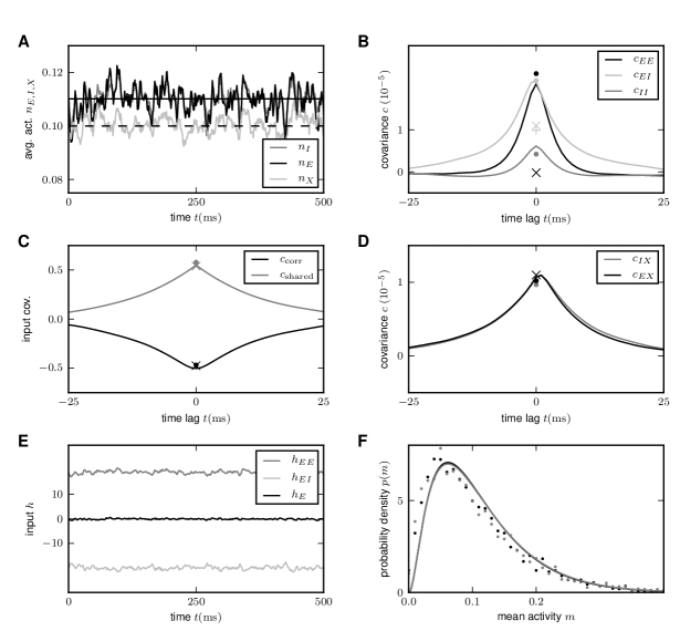
Figure 6: Activity in a network of $3N=3\times 8192$ binary neurons as described in [49], with $J_{EE}=5/\sqrt{N}$, $J_{EI}=-10/\sqrt{N}$, $J_{IE}=5/\sqrt{N}$, $J_{II}=-9/\sqrt{N}$, $J_{EX}=5/\sqrt{N}$, $J_{IX}=4/\sqrt{N}$. Number $K$ of synaptic inputs binomially distributed as $K\sim B(N,p)$, with connection probability $p=0.2$. A Population averaged activity (black $E$, gray $I$, light gray $X$). Analytical prediction (5) for the mean activities $m_{E}=m_{I}$ (dashed horizontal line) and numerical solution of mean field equation (7) (solid horizontal line). B Cross correlation between excitatory neurons (black curve), between inhibitory neurons (gray curve), and between excitatory and inhibitory neurons (light gray curve) obtained from simulation. St. Andrew’s Crosses show the theoretical prediction from [49, suppl. eqs. 38,39] (prediction yields $c_{EE}\simeq c_{II}\simeq-2\,10^{-7}$, so only one cross is visible). Dots show the theoretical prediction (50). The plus symbol shows the prediction for the correlation $c_{EI}$ when terms proportional to $a_{E}$ and $a_{I}$ are set to zero. C Correlation between the input currents to a pair of excitatory neurons. Contribution due to pairwise correlations $c{}_{\mathrm{corr},E}$ (black curve) and due to shared input $c_{\mathrm{shared},E}$ (gray curve). Symbols show the theoretical predictions based on [49] (crosses) and based on (50) (dots). D Similar to B, but showing the correlations between external neurons and neurons in the excitatory and inhibitory population. E Fluctuating input $h_{E}$ averaged over the excitatory population (black), separated into contributions from excitatory synapses $h_{EE}$ (gray) and from inhibitory synapses $h_{EI}$ (light gray). F Distribution of time averaged activity obtained by direct simulation (symbols) and analytical prediction (36) using the numerically evaluated self-consistent solution for the first $m_{E}\simeq m_{I}\simeq 0.11$ and second moments $q_{E}\simeq 0.019$, $q_{I}\simeq 0.018$ (38). Duration of simulation $T=100\mathrm{\,s}$, mean activity $m_{X}=0.1$, other parameters as in Figure 3.

It is easy to see that the cancellation condition (Cancellation of input correlations) does not uniquely determine the structure of correlations in an $E-I$ network. Figure 6 shows the same measures of activity as Figure 4, but for the network connectivity used in [49, their Fig. 2]. Except for $J_{II}$ and $J_{IX}$ the parameters are the same as in Figure 4. Moreover, we distributed the number of incoming connections $K$ per neuron according to a binomial distribution as in the original publication. As before, the cancellation of fluctuations on the input side is evident from Figure 6E, which is here realized by a different structure of covariances $c_{EE}\simeq c_{EI}>c_{II}$, shown in Figure 6B. The structure of correlations in a finite network is not uniquely determined by $\langle\delta h\rangle=0$, as seen in Figure 6B. As an example consider the correlation structure predicted in the limit of infinite network size [49, Supplementary material, eqs. 38-39], which also fulfills $\langle\delta h\rangle=0$, but does not coincide with the results obtained by direct simulation of the finite network. By construction and by virtue of (Cancellation of input correlations) this correlation structure, however, still fulfills the cancellation condition on the input side, as visualized in Figure 6C. We show in “Limit of infinite network size” below that this is due to the theory being valid only in the limit of infinite network size, neglecting the contribution of fluctuations of the local populations ($E$,$I$), as they appear in (50). Formally this is apparent from [49, eq. (2)], stating that fluctuations are predominantly caused by the external input, reflected in the expression $c_{EI}\propto a_{X}$. This can be demonstrated explicitly by setting $a_{E}=0$ and $a_{I}=0$ in (50), resulting in a similar prediction for $c_{EI}$, as shown in Figure 6B (plus symbol). The remaining deviation between the theories is due to the different susceptibilities $S$ used by the two approaches. Note that the full theory (50) predicts the structure of correlations with high accuracy. In summary, the cancellation condition imposes a constraint on the structure of correlations but is not sufficient as a unique determinant.

The distribution of the in-degree is an additional source of variability. It causes a distribution of the mean activity of the neurons in the network, as shown in Figure 6F. The shape of the distribution can be assessed analytically by self-consistently solving a system of equations for the first $m_{\alpha}$ (37) and second moment $q_{\alpha}$ (38) of the rate distribution [63], as described in “Influence of inhomogeneity of in-degrees”. The resulting second moments $q_{E}\simeq 0.0185$ ($0.0175$ by simulation) and $q_{I}\simeq 0.0184$ ($0.0180$ by simulation) are small compared to the mean activity $m_{E}\simeq m_{I}\simeq 0.11\ll 1$. For the prediction of the covariances shown in Figure 6B-D we employed the semi-analytical self-consistent solution to determine the variances $a_{\alpha}=m_{\alpha}-q_{\alpha}$. The difference to the approximate value $a_{\alpha}\simeq m_{\alpha}(1-m_{\alpha})<m_{\alpha}-[m_{\alpha}^{2}]$ is, however, small for low mean activity.

Limit of infinite network size

To relate the finite-size correlations presented in the previous sections to earlier studies of the dominant contribution to the correlations in the limit of infinitely large networks [49], we here take the limit $N\to\infty$. For non-homogeneous connectivity, we recover the earlier result [49] in “Inhomogeneous connectivity”. In “Homogeneous connectivity” we show that the correlations converge to a different limit than what would be expected from the idea of fast tracking.

Starting from (10) we follow [49, Supplementary] and introduce the covariances between population-averaged activities as $r_{\alpha\beta}=c_{\alpha\beta}+\delta_{\alpha\beta}\frac{a_{\alpha}}{N_{\alpha}}$, which leads to

$$2(r_{\alpha\beta}-\delta_{\alpha\beta}\frac{a_{\alpha}}{N_{\alpha}}) =\sum_{\gamma\in\{E,I,X\}}\left(w_{\alpha\gamma}r_{\gamma\beta}+w_{\beta\gamma}r_{\gamma\alpha}\right)$$

$$\sum_{\gamma\in\{E,I,X\}}\left(\underbrace{(\delta_{\alpha\gamma}-w_{\alpha\gamma})}_{\equiv m_{\alpha\gamma}}r_{\gamma\beta}+\underbrace{(\delta_{\beta\gamma}-w_{\beta\gamma})}_{\equiv m_{\beta\gamma}}r_{\gamma\alpha}\right) =2\delta_{\alpha\beta}\frac{a_{\alpha}}{N_{\alpha}}$$ (69)

$$MR+(MR)^{T} =2\mathrm{diag}(\{\frac{a_{\alpha}}{N_{\alpha}}\}).$$

The general solution of the continuous Lyapunov equation stated in the last line can be obtained by projecting onto the set of left-sided eigenvectors of $M$ (see e.g. [18] eq. 6.14). Alternatively the system of linear equations (69) may be written explicitly as

$$\underbrace{\left(\begin{array}[]{ccc}2-2w_{EE}&-2w_{EI}&0\\ -w_{IE}&2-\left(w_{EE}+w_{II}\right)&-w_{EI}\\ 0&-2w_{IE}&2-2w_{II}\end{array}\right)}_{\equiv\tilde{M}}\left(\begin{array}[]{c}r_{EE}\\ r_{EI}\\ r_{II}\end{array}\right) =\left(\begin{array}[]{cc}2w_{EX}&0\\ w_{IX}&w_{EX}\\ 0&2w_{IX}\end{array}\right)\left(\begin{array}[]{c}r_{EX}\\ r_{IX}\end{array}\right)+2\left(\begin{array}[]{c}\frac{a_{E}}{N_{E}}\\ 0\\ \frac{a_{I}}{N_{I}}\end{array}\right)$$ (84)

$$\left(\begin{array}[]{cc}2-w_{EE}&-w_{EI}\\ w_{IE}&2-w_{II}\end{array}\right)\left(\begin{array}[]{c}r_{EX}\\ r_{IX}\end{array}\right) =\left(\begin{array}[]{c}w_{EX}\\ w_{IX}\end{array}\right)\frac{a_{X}}{N_{X}}.$$ (91)

The solution of the latter equation is given by (31), so $r_{\alpha X}\propto\frac{a_{X}}{N_{X}}$. We observe that the right hand side of the first line in (84) contains again two source terms, those corresponding to fluctuations caused by the external drive (proportional to $r_{\alpha X}\propto\frac{a_{X}}{N_{X}}$) and those due to fluctuations generated within the network (proportional to $a_{E}$ or $a_{I}$). This motivates our definition of the two contributions $r_{\alpha\beta}^{\mathrm{ext.}}$ and $r_{\alpha\beta}^{\mathrm{int.}}$ as

$$\tilde{M\,}\left(\begin{array}[]{c}r_{EE}^{\mathrm{ext.}}\\ r_{EI}^{\mathrm{ext.}}\\ r_{II}^{\mathrm{ext.}}\end{array}\right) =\left(\begin{array}[]{cc}2w_{EX}&0\\ w_{IX}&w_{EX}\\ 0&2w_{IX}\end{array}\right)\left(\begin{array}[]{c}r_{EX}\\ r_{IX}\end{array}\right)$$ (100)

$$\tilde{M}\,\left(\begin{array}[]{c}r_{EE}^{\mathrm{int.}}\\ r_{EI}^{\mathrm{int.}}\\ r_{II}^{\mathrm{int.}}\end{array}\right) =2\left(\begin{array}[]{c}\frac{a_{E}}{N_{E}}\\ 0\\ \frac{a_{I}}{N_{I}}\end{array}\right),$$ (107)

which allows us to write the full solution of (84) as $r_{\alpha\beta}=r_{\alpha\beta}^{\mathrm{ext.}}+r_{\alpha\beta}^{\mathrm{int.}}$. We use the superscripts $\mathrm{ext.}$ and $\mathrm{int.}$ to indicate the driving sources of the fluctuations coming from outside the network ($\mathrm{ext.}$ driven by $a_{X}$) and coming from within the network ($\mathrm{int.}$ driven by $a_{E}$ and $a_{I}$).

Inhomogeneous connectivity

In the following we assume inhomogeneous connectivity, meaning that the synaptic amplitudes not only depend on the type of the sending neuron but also on the receiving neuron, such that the matrix $\{J_{\alpha\beta}\}$ is invertible. In the limit of large networks with $|w_{\alpha\beta}|\gg 1$ the solution (31) can be approximated as

$$\left(\begin{array}[]{c}c_{EX}\\ c_{IX}\end{array}\right)=\left(\begin{array}[]{c}r_{EX}\\ r_{IX}\end{array}\right) \simeq \left(\begin{array}[]{cc}w_{EE}&w_{EI}\\ w_{IE}&w_{II}\end{array}\right)^{-1}\left(\begin{array}[]{c}w_{EX}\\ w_{IX}\end{array}\right)\frac{a_{X}}{N_{X}}\equiv\left(\begin{array}[]{c}A_{E}\\ A_{I}\end{array}\right)\frac{a_{x}}{N_{x}},$$

where the definitions of $A_{E}$ and $A_{I}$ correspond to the ones of [49] if the susceptibility $S$ is the same for all populations. Solving the first system of equations (100) leads to

$$r_{\alpha\beta}^{\mathrm{ext.}} \simeq A_{\alpha}A_{\beta}\frac{a_{X}}{N_{X}},$$

where we again assumed that $|w_{\alpha\beta}|\gg 1$ and therefore neglected the term $2$ in the sums on the diagonal of the matrix $\tilde{M}$ (84). Hence the covariance due to $r_{\alpha\beta}^{\mathrm{ext.}}$ is

$$c_{\alpha\beta}^{\mathrm{ext.}} =r_{\gamma\beta}^{\mathrm{ext.}}-\delta_{\alpha\beta}\frac{a_{\alpha}}{N_{\alpha}}$$ (109)

$$\simeq A_{\alpha}A_{\beta}\frac{a_{X}}{N_{X}}-\delta_{\alpha\beta}\frac{a_{\alpha}}{N_{\alpha}}\propto N^{-1}.$$

The latter equation is the solution given in [49, Supplementary, eqs. (38)-(39) ]. The form of the equation shows that this contribution is due to fluctuations of the population activity driven by the external input, exhibited by the factor $a_{X}$ driving $r_{\alpha\beta}^{\mathrm{ext.}}$, where the intrinsic contribution of the single cell autocorrelations is subtracted. The quantities $A_{E}$ and $A_{I}$ contain the effect of the recurrence on these externally applied fluctuations and are independent of network size, so $c^{\mathrm{ext.}}$ decays with $N^{-1}$ as shown in Figure 7A (dashed curve).

The second contribution $r^{\mathrm{int.}}$ given by the solution of (107) is driven by the intrinsically generated fluctuations. As the network tends to infinity, this contribution vanishes faster than $r^{\mathrm{ext.}}$, because the coupling matrix grows as $\tilde{M}\propto w\propto\sqrt{N}$. So the term $r^{\mathrm{int.}}$ is a correction to (109) of the order $N^{-\frac{3}{2}}$. This faster decay can be observed at large network sizes in Figure 7A (dotted curve). For finite networks of natural size, however, this term determines the structure of the correlations. For the parameters chosen in [49] in particular, the contribution $r^{\mathrm{int.}}$ dominates in networks up to about $10^{7}$ neurons (Figure 7A).

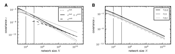
Figure 7: Scaling the network size to infinity. Comparison of the solution of (50) (solid) to the contribution of the leading order in $1/N$ (dashed). Gray coded are the different pairs of covariances, black ($c_{EE}$), mid gray ($c_{II}$), light gray ($c_{EI}$). A Network as in [49] with non-homogeneous synaptic coupling as in Figure 6. The dashed curve is given by the leading order term $c_{\alpha\beta}^{\mathrm{ext.}}=r_{\alpha\beta}^{\mathrm{ext.}}-\delta_{\alpha\beta}\frac{a_{\alpha}}{N_{\alpha}}\propto N^{-1}$ (109) and [49, eqs. (38)-(39)] driven by external fluctuations, the dotted curve is the next order term $r^{\mathrm{intr.}}\propto N^{-\frac{3}{2}}$ (107), driven by intrinsic fluctuations generated by the excitatory and inhibitory population. The dashed curve is not shown for networks smaller than $\sim 10^{6}$ neurons as it assumes negative values. Relative error of the theory with respect to simulation at $100,000$ neurons is $73$ percent. The solid curve is the full solution of (50) $c_{\alpha\beta}=r_{\alpha\beta}^{\mathrm{ext.}}+r_{\alpha\beta}^{\mathrm{intr.}}-\delta_{\alpha\beta}\frac{a_{\alpha}}{N_{\alpha}}$. The relative error at $100,000$ neurons is $16$ percent. Symbols show direct simulations. B Network with homogeneous connectivity, as in Figure 4. Same symbol code as in A. Both contributions $c_{\alpha\beta}^{\mathrm{ext.}}\propto N^{-1}$ (100) and $r^{\mathrm{intr.}}\propto N^{-1}$ (107) show the same scaling (136). Note that for the parameters here $c_{\alpha\alpha}^{\mathrm{ext.}}\simeq 0$, so the only dashed curve shown is $c_{EI}^{\mathrm{ext.}}$. Symbols indicate the results of direct simulations; vertical lines are included to guide the eye.

Homogeneous connectivity

In the previous section we showed that in agreement with [49] the leading order term $\propto N^{-1}$ dominates the limit of infinitely large networks and yields practically useful results for random networks of about $N\geq 10^{8}$ neurons. Here we will extend the theory to homogeneous connectivity, where the synaptic weights only depend on the type of the sending neuron, i.e. all $J_{\alpha E}=J_{\alpha X}=J$ and $J_{\alpha I}=-gJ$ are the same for all $\alpha$. The matrix

$$J\left(\begin{array}[]{cc}1&-g\\ 1&-g\end{array}\right)$$ (112)

is hence not invertible and the theory in “Inhomogeneous connectivity” not directly applicable. Note that assuming fast tracking here, which for inhomogeneous connectivity is a consequence of the correlation structure in the $N\to\infty$ limit [49, eq. (2)], due to the degenerate rows of the connectivity here yields

$$m_{E}(t)=m_{I}(t) =A\,m_{X}(t)$$

$$A =\frac{1}{g-1}.$$ (113)

Here such an assumption will lead to a wrong result, if $A$ is naively inserted into equation (109) or equivalently into [49, Supplementary, eqs. (38)-(39)]. In particular, for the given parameters $g-1=1$ and with the homogeneous activity (and $a_{x}=a_{E}=a_{I}$) the cross covariances $c_{\alpha\alpha}$ are predicted to approximately vanish $c_{\alpha\alpha}\simeq 0$. This failure could have been anticipated based on the observation that the tracking does not hold in this case, as observed in Figure 4A. We therefore need to extend the theory for infinite-sized networks with homogeneous connectivity.

To this end we write (50) explicitly for the homogeneous network using $a_{E}=a_{I}=a=(1-m)\,m$. We see from (50) that $c_{EX}=c_{IX}$ and $c_{EI}=c_{IE}=\frac{1}{2}(c_{EE}+c_{II})$ and introduce $w_{\alpha E}=w$, $w_{\alpha I}=-gw$, $N_{E}=N_{I}=N$ to obtain

$$\left(2-w(1-g)\right)c_{EX} = w\,\frac{a_{X}}{N_{X}}$$ (114)

$$c_{EX} = \frac{1}{2+w(g-1)}\,w\,\frac{a_{X}}{N_{X}}$$

$$\left[\mathbf{2}-w\left(\begin{array}[]{cc}2-g&-g\\ 1&1-2g\end{array}\right)\right]\left(\begin{array}[]{c}c_{EE}\\ c_{II}\end{array}\right) = 2\frac{w}{N}\,a\,\left(\begin{array}[]{c}1\\ -g\end{array}\right)+2w\,c_{EX}\left(\begin{array}[]{c}1\\ 1\end{array}\right)$$ (123)

$$w = K\,J\,S(\mu,\sigma).$$

For sufficiently large networks, we can neglect the $2\ll w$ on the left hand side of (114) to obtain

$$c_{EX}=c_{IX} =\frac{1}{g-1}\,\frac{a_{X}}{N_{X}}$$

and hence the second equation, again neglecting the $\mathbf{2}\ll w$ on the left hand side, leads to

$$\left(\begin{array}[]{c}c_{EE}\\ c_{II}\end{array}\right) =\left(\begin{array}[]{c}c_{EE}^{\mathrm{0}}\\ c_{II}^{0}\end{array}\right)+\left(\begin{array}[]{c}c_{EE}^{1}\\ c_{II}^{\mathrm{1}}\end{array}\right)$$ (130)

$$c_{EE}^{0}=c_{II}^{0} \simeq\frac{1}{g-1}\,\frac{a_{X}}{N_{X}}$$

$$\left(\begin{array}[]{c}c_{EE}^{\mathrm{1}}\\ c_{II}^{\mathrm{1}}\end{array}\right) \simeq\frac{1}{(g-1)^{2}}\,\left(\begin{array}[]{c}-1+2g+g^{2}\\ 1+2g-g^{2}\end{array}\right)\,\frac{a}{N}.$$ (135)

This result shows explicitly the two contributions to the correlations due to external fluctuations ($c^{0}$) and due to intrinsic fluctuations ($c^{1}$), respectively. In contrast to the case of inhomogeneous connectivity, both contributions decay as $N^{-1}$, so the external drive does not provide the leading contribution even in the limit $N\to\infty$. Note also that we may write this result in a similar form as for the inhomogeneous connectivity, as

$$c_{\alpha\beta}^{\mathrm{ext.}} \simeq c_{\alpha\beta}^{0}-\delta_{\alpha\beta}\frac{a_{\alpha}}{N_{\alpha}}$$

$$=A\frac{a_{X}}{N_{X}}-\delta_{\alpha\beta}\frac{a_{\alpha}}{N_{\alpha}}$$ (136)

$$r_{\alpha\beta}^{\mathrm{int.}} \simeq c_{\alpha\beta}^{1}+\delta_{\alpha\beta}\frac{a_{\alpha}}{N_{\alpha}}$$

$$\left(\begin{array}[]{c}r_{EE}^{\mathrm{int.}}\\ r_{II}^{\mathrm{int.}}\end{array}\right) =\frac{2}{(g-1)^{2}}\,\left(\begin{array}[]{c}g^{2}\\ 1\end{array}\right)\,\frac{a}{N},$$ (141)

with $A$ given by (113). Here, $c^{\mathrm{ext.}}\propto N^{-1}$ has the same form as the solution [49, eqs. (38)-(39)] originating from external fluctuations, but $r^{\mathrm{int.}}\propto N^{-1}$ is still a contribution of same order of magnitude. The susceptibility $S$ has been eliminated from these expressions and hence only structural parameters remain, analogous to the solution [49, eqs. (38)-(39)]. The two contributions $c^{\mathrm{ext.}}=r^{\mathrm{ext.}}-\delta_{\alpha\beta}\frac{a_{\alpha}}{N_{\alpha}}$ and $r^{\mathrm{int.}}$ given by the non-approximate solution of (100) and (107), respectively, are shown together with their sum and with results from direct simulations in Figure 7B. For the given network parameters, the contribution of intrinsic correlations dominates across all network sizes, because $c_{\alpha\alpha}^{\mathrm{ext.}}\simeq 0$, as $A=1$, and all $N_{\alpha}$ and $a_{\alpha}$ are approximately identical for $\alpha\in\{E,I,X\}$. The splitting between the covariances of different types scales proportional to the absolute value $\propto N^{-1}$, so even at infinite network size the differences between the covariances stays relatively the same.

The underlying reason for the qualitatively different scaling of the intrinsically generated correlations $c^{\mathrm{int.}}\propto N^{-1}$ for homogeneous connectivity compared to $c^{\mathrm{int.}}\propto N^{-\frac{3}{2}}$ for inhomogeneous connectivity is related to the one vanishing eigenvalue of the effective connectivity matrix (112). The zero eigenvalue belongs to the eigenvector $(g,1)^{T}$, meaning excitation and inhibition may in this eigendirection fluctuate freely without sensing any negative feedback through the connectivity, reflected in the last line in (136). These fluctuations are driven by the intrinsically generated noise of the stochastic update process and hence contribute notably to the correlations in the network.

In summary, the two examples “Inhomogeneous connectivity” and “Homogeneous connectivity” are both inhibition-dominated ($g>1$) networks that show small correlations on the order $\frac{a}{N}$ at finite size $N$. Only in the limit of infinitely large networks with inhomogeneous connectivity is $c^{\mathrm{ext.}}$ the dominant contribution that can be related to fast and perfect tracking of the external drive. At finite network sizes, the contribution $c^{\mathrm{int.}}$ is generally not negligible and may be dominant. Therefore fast tracking cannot be the explanation for small correlations in these networks. Note that there is a difference in the line of argument used in the main text of [49] and its mathematical supplement: While the main text advocates fast tracking as the underlying mechanism explaining small correlations, in the mathematical supplement fast tracking is found as a consequence of the theory of correlations in the limit of infinite-sized networks and under the stated prerequisites, in line with the calculation presented above.

Influence of connectivity on the correlation structure

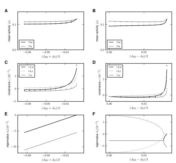
Figure 8: Connectivity structure determines correlation structure. In the left column (A,C,E) $c_{1}=(J_{EE}+J_{II})/2$ is the independent variable, in the right column (B,D,F) $c_{2}=(J_{EE}-J_{II})/2$. A,B Mean activity in the network as a function of the structural parameters $c_{1}$ and $c_{2}$, respectively. C,D Correlations averaged over pairs of neurons. Dots obtained from direct simulation, solid curves given by theory (50) E,F Eigenvalues (142) of the population-averaged connectivity matrix; solid curves show the real part, dashed curves the imaginary part.

Comparing Figure 4B and Figure 6B, the structure of correlations is obviously different. In Figure 4B, the structure is $c_{EE}>c_{EI}>c_{II}$, whereas in Figure 6B the relation is $c_{EI}\simeq c_{EE}>c_{II}$. The only difference between these two networks are the coupling strengths $J_{II}$ and $J_{IX}$. In the following we derive a more complete picture of the determinants of the correlation structure. In order to identify the parameters that influence the fluctuations in these networks, it is instructive to study the mean-field equation for the population-averaged activities. Linearizing (39) for small deviations $\delta n_{\alpha}=n_{\alpha}-m_{\alpha}$ of the population-averaged activity $n_{\alpha}$ from the fixed point $m_{\alpha}$, for large networks with $N>K_{\alpha\beta}\gg 1$ the dominant term is proportional to the change of the mean $\delta\mu_{\alpha}=\sum_{\beta}(JK)_{\alpha\beta}\delta n_{\beta}$, because the standard deviation $\delta\sigma_{\alpha}$ is only proportional to $\sqrt{K_{\alpha\beta}}$. To linear order we hence have a coupled set of two differential equations (66). The dynamics of this coupled set of linear differential equations is determined by the two eigenvalues of the effective connectivity

$$\lambda_{1,2} = \mathrm{eig}\left(\{w_{\alpha\beta}\}\right)$$ (142)

$$= \frac{w_{EE}+w_{II}}{2}\pm\sqrt{\left(\frac{w_{EE}-w_{II}}{2}\right)^{2}+w_{EI}w_{IE}}.$$

Due to the presence of the leak term on the left hand side of (66), the fixed point rate is stable only if the real parts of the eigenvalues $\lambda_{1,2}$ are both smaller than $1$. In the network with identical input statistics for all neurons the fluctuating input is characterized by the same mean and variance $(\mu,\sigma^{2})$ for each neuron. For homogeneous neuron parameters the susceptibility $S_{\alpha}=S$ is hence the same for both populations $\alpha\in\{E,I\}$. If further the number of synaptic afferents is the same $K_{\alpha\beta}=K$ for all populations, the eigenvalues can be expressed by those of the original connectivity matrix as

$$\frac{\lambda_{1,2}}{S(\mu,\sigma)K} = \frac{J_{EE}+J_{II}}{2}\pm\sqrt{\left(\frac{J_{EE}-J_{II}}{2}\right)^{2}+J_{EI}J_{IE}}$$

$$= c_{1}\pm\sqrt{c_{2}^{2}+J_{EI}J_{IE}},$$

where we defined the two parameters $c_{1}$ and $c_{2}$ which control the location of the eigenvalues. In the left column of Figure 8 we keep $J_{EI}$, $J_{IE}$, and $c_{2}$ constant and vary $c_{1}\in[-c_{2},-\sqrt{c_{2}^{2}+J_{EI}J_{IE}}]$, where we choose the maximum value by the condition $\lambda_{1}<0$ and the minimum value by the condition that $J_{EE}\geq 0$ and $J_{II}\leq 0$, leading to $c_{1}+c_{2}\geq 0$ and $c_{1}-c_{2}\leq 0$, both fulfilled if $-c_{2}\leq c_{1}\leq c_{2}$. Varying $c_{2}$ in the right column of Figure 8, the bounds are given by the same condition that $J_{EE}\geq 0$ and $J_{II}\leq 0$, so $c_{2}\geq 0$, and the condition for the larger eigenvalue to stay below or equal $0$, so $c_{2}\in[0,\sqrt{c_{1}^{2}-J_{EI}J_{IE}}]$. In order for the network to maintain similar mean activity, we choose the threshold of the neurons such that the cancellation condition $0=\sum_{\beta\in\{E,I,X\}}(KJ)_{\alpha\beta}m_{\beta}-\theta$ is fulfilled for $m_{\beta}=0.1$. The resulting average activity is close to this desired value of $0.1$ and agrees well to the analytical prediction (39), as shown in Figure 8A, B.

The right-most point in both columns of Figure 8 where one eigenvalue vanishes $\lambda_{1}=0$, results in the same connectivity structure. This is the case for the connectivity with the symmetry $J_{EE}=J_{IE}=J$ and $J_{II}=J_{EI}=-gJ$ (cf. Figure 4), because in this case the population averaged connectivity matrix has two linearly dependent rows, hence a vanishing determinant and thus an eigenvalue $0$. As observed in Figure 8C,D at this point the absolute magnitude of correlations is largest. This is intuitively clear as the network has a degree of freedom in the direction of the eigenvector $v_{1}=(g,1)^{T}$ belonging to the vanishing eigenvalue $\lambda_{1}=0$. In this direction the system effectively does not feel any negative feedback, so the evolution is as if the connectivity would be absent. Fluctuations in this direction hence become large and are only damped by the exponential relaxation of the neuronal dynamics, given by the left hand side of (66). The time constant of these fluctuations is then solely determined by the time constant of the single neurons, as seen in Figure 4B. From the coefficients of the eigenvector we can further conclude that the fluctuations of the excitatory population are stronger by a factor $g$ than those of the inhibitory population, explaining why $c_{EE}>c_{II}$, and that both populations fluctuate in-phase, so $c_{EI}>0$, (Figure 8C,D, right most point). Moving away from this point, Figure 8C,D both show that the magnitude of correlations decreases. Comparing the temporal structures of Figure 4B and Figure 6B shows that also the time scale of fluctuations decreases. The two structural parameters $c_{1}$ and $c_{2}$ affect the eigenvalues of the connectivity in a distinct manner. Changing $c_{1}$ merely shifts the real part of both eigenvalues, but leaves their relative distance constant, as seen in Figure 8E. For smaller values of $c_{1}$ the coupling among excitatory neurons becomes weaker, so their correlations are reduced. At the left most point in Figure 8C the coupling within the excitatory population vanishes, $J_{EE}=0$. Changing the parameter $c_{2}$ has a qualitatively different effect on the eigenvalues, as seen in Figure 8F. At $c_{2}=\sqrt{|J_{EI}J_{IE}|}$, the two real eigenvalues merge and for smaller $c_{2}$ they turn into a conjugate complex pair. At the left-most point $J_{EE}-J_{II}=0$, so both couplings within the populations vanish $J_{EE}=J_{II}=0$. The system then only has coupling from $E$ to $I$ and vice versa. The conjugate complex eigenvalues show that the population activity of the system has oscillatory solutions. This is also called the PING (pyramidal - inhibitory - gamma) mechanism of oscillations in the gamma-range [10]. Figure 8C,D show that for most connectivity structures the correlation structure is $c_{EI}>c_{EE}>c_{II}$, in contrast to our previous finding [58], where we studied the symmetric case (the right-most point), at which the correlation structure is $c_{EE}>c_{EI}>c_{II}$. The comparison of the direct simulation to the theoretical prediction (50) in Figure 8C,D shows that the theory yields an accurate prediction of the correlation structure for all connectivity structures considered here.

Discussion

The present work explains the observed pairwise correlations in a homogeneous random network of excitatory and inhibitory binary model neurons driven by an external population of finite size.

On the methodological side the work is similar to the approach taken in the work of Renart et al. [49], that starts from the microscopic Glauber dynamics of binary networks with dense and strong synaptic coupling $J\propto N^{-\frac{1}{2}}$ and derives a set of self-consistent equations for the second moment of the fluctuations in the network. As in the earlier work [49], we take into account the fluctuations due to the balanced synaptic noise in the linearization of the neuronal response [49, 19] rather than relying on noise intrinsic to each neuron, as in the work by Ginzburg and Sompolinsky [18]. Although the theory by Ginzburg and Sompolinsky [18] was explicitly derived for binary networks that are densely, but weakly coupled, i.e. the number of synapses per neuron is $\propto N$ and synaptic amplitudes scale as $J\propto N^{-1}$, identical equations result for the case of strong coupling, where the synaptic amplitudes decay slower than $N^{-1}$ [49]. The reason for both weakly and strongly coupled networks to be describable by the same theory lies in the self-regulating property of binary neurons: Their susceptibility (called $S$ in the present work) inversely scales with the fluctuations in the input, $S\propto\sigma^{-1}\propto J^{-1}$, such that $JS$ and hence correlations are independent of synaptic amplitude $J$ [19]. A difference between the work of Ginzburg and Sompolinsky [18] and the work of Renart et al. [49] is, however, that the first authors assume all correlations to be equally small $\propto N^{-1}$, whereas the latter show that the distribution of correlations is wider than their mean due to the variability in the connectivity, in particular the varying number of common inputs. The theory yields the dominant contribution to the mean value of this distribution scaling as $N^{-1}$ in the limit of infinite network size. Although the asynchronous state of densely coupled networks has been described earlier [62, 63] by a mean-field theory neglecting correlations, the main achievement of the work by Renart et al. [49] must be seen as demonstrating that the formal structure of the theory of correlations indeed admits a solution with low correlations of order $N^{-1}$ and that such a solution is accompanied by the cancellation of correlations between the inputs to pairs of neurons. The latter authors employed an elegant scaling argument, taking the network size and hence the coupling to infinity, to obtain their results. In contrast, here we study these networks at finite size and obtain a theoretical prediction in good agreement with direct simulations in a large range of biologically relevant networks sizes. We further extend the framework of correlations in binary networks by an iterative procedure taking into account the finite-size fluctuations in the mean-field solution to determine the working point (mean activity) of the network. We find that the iteration converges to predictions for the covariance with higher accuracy than the previous method.

Equipped with these methods we investigate a network driven by correlated input due to shared afferents supplied by an external population. The analytical expressions for the covariances averaged over pairs of neurons show that correlations have two components that linearly superimpose, one caused by intrinsic fluctuations generated within the local network and one caused by fluctuations due to the external population. The size $N_{X}$ of the external population controls the strength of the correlations in the external input. We find that this external input causes an offset of all pairwise correlations, which decreases with increasing external population size in proportion to the strength of the external correlations ($\propto 1/N_{X}$). The structure of correlations within the local network, i.e. the differences between correlations for pairs of neurons of different types, is mostly determined by the intrinsically generated fluctuations. These are proportional to the population-averaged variances $a_{E}$ and $a_{I}$ of the activity of the neurons in the local network. As a result, the structure of correlations is mostly independent of the external drive, even for the limiting case of an infinitely large external population $N_{X}\rightarrow\infty$ or if the external drive is replaced by a DC signal with the same mean. For the other extreme, when the size of the external population equals the number of external afferents, $N_{X}=K$, all neurons receive an exactly identical external signal. We show that the mechanism of decorrelation [49, 58] still holds for these strongly correlated external signals. The resulting correlation within the network is much smaller than expected given the amount of common input. In contrast to an earlier explanation [49], which invokes the network’s fast tracking of the external drive [62, 63] as the cause of small correlations, we here show that the cancellation of correlations between the inputs to pairs of neurons is equivalent to a suppression of fluctuations of the population-averaged input due to negative feedback. This argument is in line with the earlier explanation that correlations are suppressed by negative feedback on the population level [58]. Such dominant negative feedback is a fundamental requirement for the network to stabilize its activity in the balanced state [62]. We further show that the cancellation of input correlations does not uniquely determine the structure of correlations; different structures of correlations lead to the same cancellation of correlations between the summed inputs. The cancellation of input correlations therefore only constitutes a constraint for the pairwise correlations in the network. This constraint is trivially fulfilled if the network shows perfect tracking of external input, which is equivalent to completely vanishing input fluctuations [49]. The correlation structure in finite-sized networks is in general different from this limit, but fulfills the constraint imposed by the cancellation of input correlations.

Performing the limit $N\to\infty$ we distinguish two cases. For an invertible connectivity matrix, we recover the result by [49], that in the limit of infinite network size correlations are dominated by tracking of the external signal and intrinsically generated fluctuations can be neglected; the resulting expressions for the correlations within the network [49, Supplementary, eqs. 38,39] are lacking the locally generated fluctuations as additional sources. However, note that the intermediate result [49, Supplementary, eqs. 31,33] is identical to [18, eq. 6.8] and to (9) and contains both contributions.

The convergence of the correlation structure to the limiting theory appears to be slow. For the parameters given in [49], quantitative agreement is achieved at around $10^{8}$ neurons, which is beyond the scale up to which random networks are good models for cortical networks. For the range of biologically relevant network sizes the correlation structure is dominated by intrinsic fluctuations. One should note that the lines of argument used in the main text of [49] and in its mathematical supplement are different. The main text starts at the observation that for an invertible connectivity matrix and in the inhibition-dominated regime the network activity exhibits fast-tracking. The authors then argue that hence positive correlations between excitatory and inhibitory synaptic currents are responsible for the decorrelation of network activity. The mathematical supplement, however, first derives the leading term for the pairwise correlations in the network in the limit of infinite-sized networks [49, Supplementary, eqs. 38,39] and then shows that fast tracking and the cancellation of input correlations are both consequences. For a singular matrix, as for example resulting from statistically identical inputs to excitatory and inhibitory neurons, the contributions of external and intrinsic fluctuations both scale as $N^{-1}$. Hence the intrinsic contribution cannot be neglected even in the limit $N\to\infty$. At finite network size the observed structure of correlations generally contains contributions from both intrinsic and external fluctuations, still present in the intermediate result [49, Supplementary, eqs. 31,33] and in [18, eq. 6.8] and (9). In particular, the external contribution dominating in infinite networks with invertible connectivity may be negligible at finite network size. We therefore conclude that the mechanism determining the correlation structure in finite networks cannot be deduced from the limit $N\to\infty$ and is not given by fast tracking of the external signal. Fast tracking is rather a consequence of negative feedback.

For a common but special choice of network connectivity where the synaptic weights depend only on the type of the source but not the target neuron, i.e. $J_{EE}=J_{IE}$ and $J_{EI}=J_{II}$ [7], we show that the locally generated fluctuations and correlations are elevated and that the activity only loosely tracks the external input. The resulting correlation structure is $c_{EE}>c_{EI}>c_{II}$. To systematically investigate the dependence of the correlation structure on the network connectivity, it proves useful to parameterize the structure of the network by two measures differentially controlling the location of the eigenvalues of the connectivity matrix. We find that for a wide parameter regime the correlations change quantitatively, but the correlation structure $c_{EI}>c_{EE}>c_{II}$ remains invariant. The qualitative comparison with experimental observations of [14] hence only constrains the connectivity to be within the one or the other parameter regime.

The networks we study here are balanced networks in the original sense as introduced in [62], that is to say they are inhibition-dominated and the balance of excitatory and inhibitory currents on the input side to a neuron arises as a dynamic phenomenon due to dominance of negative feedback that stabilizes the mean activity. A network with a balance of excitation and inhibition built into the connectivity of the network on the other hand would correspond in our notation to setting $J_{\alpha E}=-J_{\alpha I}$ for both receiving populations $\alpha\in\{E,I\}$, assuming identical sizes for the excitatory and the inhibitory population. The network activity is then no longer stabilized by negative feedback, because the mean activities $m_{E}$ and $m_{I}$ can freely co-fluctuate, $m_{E}=m_{E}^{0}+\delta m$ and $m_{I}=m_{I}^{0}+\delta m$, without affecting the input to other cells: $J_{\alpha E}m_{E}+J_{\alpha I}m_{I}$ is independent of $\delta m$. Mathematically this amounts to a two-fold degenerate vanishing eigenvalue of the effective connectivity matrix. The resulting strong fluctuations would have to be treated with different methods than presented here and would lead to strong correlations. The current work assumes that fluctuations are sufficiently small so that their effect can be treated in linear response theory, restricting the expressions to sufficiently asynchronous and irregular network states. This limitation arises from the linearization procedure, which approximates the summed synaptic input by a Gaussian random variable. The deviations of the theory from direct simulations are stronger at lower mean activity, when the synaptic input fluctuates in the non-linear part of the effective transfer function. The best agreement of theory and simulation is hence obtained for a mean population activity close to $\frac{1}{2}$, where $1$ means all neurons are active.

For simplicity in most parts of this work we consider networks where neurons have a fixed in-degree. In large homogeneous random networks this is often a good approximation, because the mean number of connections is $pN\propto N$, and its standard deviation $\sqrt{Np(1-p)}\propto\sqrt{N}$ declines relative to the mean. Taking into account distributed synapse numbers and the resulting distribution of the mean activity in Figure 6 and Figure 7A shows that the results are only marginally affected for low mean activity. The impact of the activity distribution on the correlation structure is more pronounced at higher mean activity, where the second moment of the activity distribution has a notable effect on the population-averaged variance.

The presented work is closely related to our previous work on the correlation structure in spiking neuronal networks [58] and indeed was triggered by the review process of the latter. In [58], we exclusively studied the symmetric connectivity structure, where excitatory and inhibitory neurons receive the same input on average. The results are qualitatively the same as those shown in Figure 4. A difference though is, that the external input in [58] is uncorrelated, whereas here it originates from a common finite population. The cancellation condition for input correlations, also observed in vivo [40], holds for spiking networks as well as for the binary networks studied here. For both models, negative feedback constitutes the essential mechanism underlying the suppression of fluctuations at the population level. This can be explained by a formal relationship between both models (see [20]).

Our theory presents a step towards an understanding of how correlated neuronal activity in local cortical circuits is shaped by recurrence and inputs from other cortical and thalamic areas. The correlation between membrane potentials of pairs of neurons in somatosensory cortex of behaving mice is dominated by low-frequency oscillations during quiet wakefulness. If the animal starts whisking, these correlations significantly decrease, even if the sensory nerve fibers are cut, suggesting an internal change of brain state [48]. Our work suggests that such a dynamic reduction of correlation could come about by modulating the effective negative feedback in the network. A possible neural implementation is the increase of tonic drive to inhibitory interneurons. This hypothesis is in line with the observed faster fluctuations in the whisking state [48]. Further work is needed to verify if such a mechanism yields a quantitative explanation of the experimental observations.

The network where the number of incoming external connections per neuron equals the size of the external population, cf. Figure 3 $N_{x}=K$, can be regarded as a setting where all neurons receive an identical incoming stimulus. The correlations between this signal and the responses of neurons in the local network (Figure 3C) are smaller than in an unconnected population without local negative feedback. This can formally be seen from (66), because negative eigenvalues of the recurrent coupling dampen the population response of the system. This suppression of correlations between stimulus and local activity hence implies weaker responses of single neurons to the driving signal. Recent experiments have shown that only a sparse subset of around 10 percent of the neurons in S1 of behaving mice responds to a sensory stimulus evoked by the active touch of a whisker with an object [11]. The subset of responding cells is determined by those neurons in which the cell specific combination of activated excitatory and inhibitory conductances drives the membrane potential above threshold. Our work suggests that negative feedback mediated among the layer 2/3 pyramidal cells, e.g. through local interneurons, should effectively reduce their correlated firing. In a biological network the negative feedback arrives with a synaptic delay and effectively reduces the low-frequency content [58]. The response of the local activity is therefore expected to depend on the spectral properties of the stimulus. Intuitively one expects responses to better lock to the stimulus for fast and narrow transients with high-frequency content. Further work is required to investigate this issue in more detail.

A large number of previous studies on the dynamics of local cortical networks focuses on the effect of the local connectivity, but ignores the spatio-temporal structure of external inputs by assuming that neurons in the local network are independently driven by external (often Poissonian) sources. Our study shows that the input correlations of pairs of neurons in the local network are only weakly affected by additional correlations caused by shared external afferents: Even for the extreme case where all neurons in the network receive exactly identical external input ($N_{x}=K$), the input correlations are small and only slightly larger than those obtained for the case where neurons receive uncorrelated external input ($N_{x}=2N$; black curve in Figure 8C). One may therefore conclude that the approximation of uncorrelated external input is justified. In general, this may however be a hasty conclusion. Tiny changes in synaptic-input correlations have drastic effects, for example, on the power and reach of extracellular potentials [34]. For the modeling of extracellular potentials, knowledge of the spatio-temporal structure of inputs from remote areas is crucial.

The theory of correlations in presence of externally impinging signals is a required building block to study correlation-sensitive synaptic plasticity [39] in recurrent networks. Understanding the emerging structure of correlations imposed by an external signal is the first step in predicting the connectivity patterns resulting from ongoing synaptic plasticity sensitive to those correlations.

References

- 1. Abeles M (1982) Local Cortical Circuits: An Electrophysiological Study. Studies of Brain Function. Berlin, Heidelberg, New York: Springer-Verlag.
- 2. Amit DJ, Brunel N (1997) Model of global spontaneous activity and local structured activity during delay periods in the cerebral cortex. Cereb Cortex 7:237–252.
- 3. Bernacchia A, Wang XJ (2013) Decorrelation by recurrent inhibition in heterogeneous neural circuits. Neural Comput 25:1732–1767.
- 4. Bi G, Poo M (1998) Synaptic modifications in cultured hippocampal neurons: Dependence on spike timing, synaptic strength, and postsynaptic cell type. J Neurosci 18:10464–10472.
- 5. Bienenstock E (1995) A model of neocortex. Network: Comput Neural Systems 6:179–224.
- 6. Binzegger T, Douglas RJ, Martin KAC (2004) A quantitative map of the circuit of cat primary visual cortex. J Neurosci 39:8441–8453.
- 7. Brunel N (2000) Dynamics of sparsely connected networks of excitatory and inhibitory spiking neurons. J Comput Neurosci 8:183–208.
- 8. Brunel N, Hakim V (1999) Fast global oscillations in networks of integrate-and-fire neurons with low firing rates. Neural Comput 11:1621–1671.
- 9. Buice MA, Cowan JD, Chow CC (2009) Systematic fluctuation expansion for neural network activity equations. Neural Comput 22:377–426.
- 10. Buzsáki G, Wang XJ (2012) Mechanisms of gamma oscillations. Annu Rev Neurosci 35:203–225.
- 11. Crochet S, Poulet JF, Kremer Y, Petersen CC (2011) Synaptic mechanisms underlying sparse coding of active touch. Neuron 69:1160–1175.
- 12. De la Rocha J, Doiron B, Shea-Brown E, Kresimir J, Reyes A (2007) Correlation between neural spike trains increases with firing rate. Nature 448:802–807.
- 13. Diesmann M, Gewaltig MO, Aertsen A (1999) Stable propagation of synchronous spiking in cortical neural networks. Nature 402:529–533.
- 14. Gentet L, Avermann M, Matyas F, Staiger JF, Petersen CC (2010) Membrane potential dynamics of GABAergic neurons in the barrel cortex of behaving mice. Neuron 65:422–435.
- 15. Gewaltig MO, Diesmann M (2007) NEST (NEural Simulation Tool). Scholarpedia 2:1430.
- 16. Gilbert CD, Wiesel TN (1983) Clustered intrinsic connections in cat visual cortex. J Neurosci 5:1116–33.
- 17. Gilson M, Burkitt AN, Grayden DB, Thomas DA, van Hemmen JL (2009) Emergence of network structure due to spike-timing-dependent plasticity in recurrent neuronal networks. I. Input selectivity - strengthening correlated input pathways. Biol Cybern 101:81–102.
- 18. Ginzburg I, Sompolinsky H (1994) Theory of correlations in stochastic neural networks. Phys Rev E 50:3171–3191.
- 19. Grytskyy D, Tetzlaff T, Diesmann M, Helias M (2013) Invariance of covariances arises out of noise. AIP Conf Proc 1510:258–262. doi:10.1063/1.4776531.
- 20. Grytskyy D, Tetzlaff T, Diesmann M, Helias M (2013) A unified view on weakly correlated recurrent networks. arXiv :1304.7945 [q–bio.NC].
- 21. Hanuschkin A, Kunkel S, Helias M, Morrison A, Diesmann M (2010) A general and efficient method for incorporating precise spike times in globally time-driven simulations. Front Neuroinform 4:113.
- 22. Hebb DO (1949) The organization of behavior: A neuropsychological theory. New York: John Wiley & Sons.
- 23. Helias M, Tetzlaff T, Diesmann M (2013) Echoes in correlated neural systems. New J Phys 15:023002.
- 24. Hertz J (2010) Cross-correlations in high-conductance states of a model cortical network. Neural Comput 22:427–447.
- 25. Hertz J, Krogh A, Palmer RG (1991) Introduction to the Theory of Neural Computation. Perseus Books.
- 26. Hopfield JJ (1982) Neural networks and physical systems with emergent collective computational abilities. Proc Natl Acad Sci USA 79:2554–2558.
- 27. Hu Y, Trousdale J, Josić K, Shea-Brown E (2013) Motif statistics and spike correlations in neuronal networks. J Stat Mech :P03012doi:10.1088/1742-5468/2013/03/P03012.
- 28. Ito J, Maldonado P, Singer W, Grün S (2011) Saccade-related modulations of neuronal excitability support synchrony of visually elicited spikes. Cereb Cortex 21:2482–2497.
- 29. Izhikevich EM (2006) Polychronization: Computation with spikes. Neural Comput 18:245–282.
- 30. Jones E, Oliphant T, Peterson P, et al. (2001). SciPy: Open source scientific tools for Python. Http://www.scipy.org/.
- 31. Kelly F (1979) Stochastic processes and reversibility. Wiley, Cambridge University Press.
- 32. Kilavik BE, Roux S, Ponce-Alvarez A, Confais J, Gruen S, et al. (2009) Long-term modifications in motor cortical dynamics induced by intensive practice. J Neurosci 29:12653–12663.
- 33. Kriener B, Tetzlaff T, Aertsen A, Diesmann M, Rotter S (2008) Correlations and population dynamics in cortical networks. Neural Comput 20:2185–2226.
- 34. Lindén H, Tetzlaff T, Potjans TC, Pettersen KH, Grün S, et al. (2011) Modeling the spatial reach of the LFP. Neuron 72:859–872.
- 35. Lindner B, Doiron B, Longtin A (2005) Theory of oscillatory firing induced by spatially correlated noise and delayed inhibitory feedback. Phys Rev E 72:061919.
- 36. Litwin-Kumar A, Chacron MJ, Doiron B (2012) The spatial structure of stimuli shapes the timescale of correlations in population spiking activity. PLoS Comput Biol 8:e1002667.
- 37. Maldonado P, Babul C, Singer W, Rodriguez E, Berger D, et al. (2008) Synchronization of neuronal responses in primary visual cortex of monkeys viewing natural images. J Neurophysiol 100:1523–1532.
- 38. Meyer C, van Vreeswijk C (2002) Temporal correlations in stochastic networks of spiking neurons. Neural Comput 14:369–404.
- 39. Morrison A, Diesmann M, Gerstner W (2008) Phenomenological models of synaptic plasticity based on spike-timing. Biol Cybern 98:459–478.
- 40. Okun M, Lampl I (2008) Instantaneous correlation of excitation and inhibition during sensory-evoked activities. Nat Neurosci 11:535–537.
- 41. Ostojic S, Brunel N, Hakim V (2009) How connectivity, background activity, and synaptic properties shape the cross-correlation between spike trains. J Neurosci 29:10234–10253.
- 42. Padmanabhan K, Urban NN (2010) Intrinsic biophysical diversity decorrelates neuronal firing while increasing information content. Nat Neurosci 13:1276–1282.
- 43. Palmer EM (1985) Graphical Evolution. Wiley.
- 44. Parga N (2013) Towards a self-consistent description of irregular and asynchronous cortical activity. J Stat Mech: Theory and Exp :P03010doi:10.1088/1742-5468/2013/03/P03010.
- 45. Pernice V, Staude B, Cardanobile S, Rotter S (2011) How structure determines correlations in neuronal networks. PLoS Comput Biol 7:e1002059.
- 46. Pernice V, Staude B, Cardanobile S, Rotter S (2012) Recurrent interactions in spiking networks with arbitrary topology. Phys Rev E 85:031916.
- 47. Potjans TC, Diesmann M (2012) The cell-type specific cortical microcircuit: Relating structure and activity in a full-scale spiking network model. Cerebral Cortex doi:doi:10.1093/cercor/bhs358. In press.
- 48. Poulet J, Petersen C (2008) Internal brain state regulates membrane potential synchrony in barrel cortex of behaving mice. Nature 454:881–885.
- 49. Renart A, De La Rocha J, Bartho P, Hollender L, Parga N, et al. (2010) The asynchronous state in cortical cicuits. Science 327:587–590.
- 50. Rosenbaum R, Josic K (2011) Mechanisms that modulate the transfer of spiking correlations. Neural Comput 23:1261–1305.
- 51. Rosenbaum R, Rubin JE, Doiron B (2013) Short-term synaptic depression and stochastic vesicle dynamics reduce and shape neuronal correlations. J Neurophysiol 109:475–484.
- 52. Rumelhart DE, McClelland JL, the PDP Research Group (1986) Parallel Distributed Processing, Explorations in the Microstructure of Cognition: Foundations, volume 1. Cambridge, Massachusetts: MIT Press.
- 53. Salinas E, Sejnowski TJ (2001) Correlated neuronal activity and the flow of neural information. Nat Rev Neurosci 2:539–550.
- 54. Shadlen MN, Newsome WT (1998) The variable discharge of cortical neurons: Implications for connectivity, computation, and information coding. J Neurosci 18:3870–3896.
- 55. Singer W, Gray C (1995) Visual feature integration and the temporal correlation hypothesis. Annu Rev Neurosci 18:555–586.
- 56. Stepanyants A, Martinez LM, Ferecskó AS, Kisvárday ZF (2009) The fractions of short- and long-range connections in the visual cortex. Proc Nat Acad Sci USA 106:3555–3560.
- 57. Sterne P (2012) Information recall using relative spike timing in a spiking neural network. Neural Comput 24:2053–2077.
- 58. Tetzlaff T, Helias M, Einevoll G, Diesmann M (2012) Decorrelation of neural-network activity by inhibitory feedback. PLoS Comput Biol 8:e1002596.
- 59. Tetzlaff T, Rotter S, Stark E, Abeles M, Aertsen A, et al. (2008) Dependence of neuronal correlations on filter characteristics and marginal spike-train statistics. Neural Comput 20:2133–2184.
- 60. Tripp B, Eliasmith C (2007) Neural populations can induce reliable postsynaptic currents without observable spike rate changes or precise spike timing. Cereb Cortex 17:1830–1840.
- 61. Trousdale J, Hu Y, Shea-Brown E, Josic K (2012) Impact of network structure and cellular response on spike time correlations. PLoS Comput Biol 8:e1002408.
- 62. van Vreeswijk C, Sompolinsky H (1996) Chaos in neuronal networks with balanced excitatory and inhibitory activity. Science 274:1724–1726.
- 63. Van Vreeswijk C, Sompolinsky H (1998) Chaotic balanced state in a model of cortical circuits. Neural Comput 10:1321–1371.
- 64. Voges N, Schüz A, Aertsen A, Rotter S (2010) A modeler’s view on the spatial structure of intrinsic horizontal connectivity in the neocortex. Progress in Neurobiology 92:277–292.
- 65. von der Malsburg C (1981) The correlation theory of brain function. Internal report 81-2, Department of Neurobiology, Max-Planck-Institute for Biophysical Chemistry, Göttingen, Germany.
- 66. Zohary E, Shadlen MN, Newsome WT (1994) Correlated neuronal discharge rate and its implications for psychophysical performance. Nature 370:140–143.