On one dimensional inverse problems arising from polarimetric measurements of nematic liquid crystals
Abstract.
We revisit the problem of determining dielectric parameters in layered nematic liquid crystals from polarimetric measurements originally introduced by Lionheart & Newton. After a detailed analysis of the model, of the scales involved, and of natural obstacles to the reconstruction of more than one dielectric parameters, we produce two simple one-dimensional inverse problems which can be studied without any expertise in liquid crystals. We then confirm that very little can be recovered about the internal configuration of smooth dielectric parameters from these measurements, and give a uniqueness result for one of the two problem, when the unknown parameter satisfies a monotonicity property. In that case, the available data can be expressed in terms of Laplace and Hankel transforms.
1. Introduction
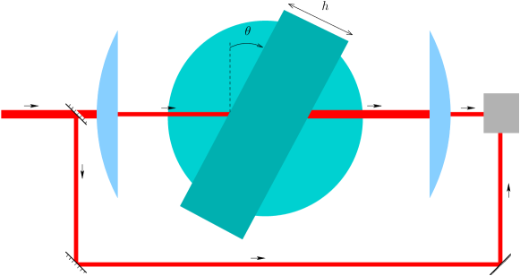
Consider the experiment sketched in Figure 1. A polarized focused laser beam is split in two beams. One beam propagates in an homogeneous medium (in light blue), and travels through a slab containing the liquid crystal (LC) cell. The transmitted beam exits on the opposite side of the slab, and enters an analyser, where it is compared to the other part of the split beam, which did not pass through the slab. The analyser delivers four real numbers, called the Stokes parameters. The LC cell is placed on a cylindrical mount, to allow variations of the incident angle of the laser in the slab. The Stokes parameters, appropriately normalized, are collected for a large range of incident angles. The purpose of this article is to study the dependence of the data on the dielectric tensor of the liquid crystal, and discuss its possible reconstruction.
The liquid crystal contained in the slab has a layered structure: the dielectric permittivity is constant and anisotropic in each layer. The magnetic permeability is a constant number. The liquid crystal is coated with thin films (polyimide, indium tin oxide…) but these thin films will not be taken into account in our study. This experiment was performed at Hewlett-Packard Laboratories, Bristol and was analysed by Lionheart & Newton [1] using a singular value decomposition approach.
To model this problem we adopt the approximation introduced in Berreman [2], following Lionheart & Newton [1]. The incident polarized laser beam in the isotropic medium in front of the liquid crystal is modelled by monochromatic plane waves incident obliquely in the (–) plane (the plane in which the experiment is sketched), with direction . The corresponding electric field has two components,
which is parallel to , and
along . To take into account possible phase differences, the amplitudes of and are complex numbers. When the incident field is polarized linearly, and are of the form and , with and .
When the incident field has a circular polarization, . The central frequency of the laser is denoted by , is the speed of light, and is the index of the isotropic medium around the slab on the wave path. We assume that within the slab, the propagating electric and magnetic fields and stay alike plane waves along the direction, and do not depend on . Thus and are modelled by the following ansatz
| (1) |
and satisfy the time-harmonic Maxwell’s equations
| (2) |
Where is the relative dielectric tensor, with constant entries outside the slab and varying as a function of within the LC cell, and and are universal constants. See Lionheart & Newton [1], Tsering-Xiao [3] and references therein for more details and discussions on this model, and Lavrentovich [4] for further insight on optical measurements of liquid crystals. Substituting (1) into (2), Maxwell’s system becomes a system of ordinary differential equations in where the unknown is the vector which satisfies
| (3) |
The Berreman vector is the tangential part of the electromagnetic fields and represents the optical field. The Berreman matrix depends on the dielectric tensor . In the outer isotropic medium, the Berreman matrix has a block diagonal structure, corresponding to the two possible polarizations of the electric field, along and . The Berreman matrix has four eigenvectors . The vectors and correspond to the incoming electric and magnetic fields, whereas the vectors and correspond to the outgoing electric and magnetic fields, see Section 2.1. The direct problem is formulated in Lionheart & Newton [1] as a transmission problem. The incident field and the transmitted field are represented by the input vector and the output vector . The reflected field is a combination of the outgoing eigenvectors and . If is the thickness of the slab, and is the transmission matrix coming from (3), the transmission problem takes the form
| (4) |
The Stokes parameters (the measured data) are
| (5) |
The questions investigated numerically in Lionheart & Newton [1] are
-
(1)
Can the dielectric tensor through the LC cell be deduced from the data?
-
(2)
How is the solution affected by the range of incident angles and input polarisations used?
-
(3)
Given the limited accuracy of the polarimeter how much information can be deduced from the data?
The goal of this paper is to address these questions analytically. In section 2 we reformulate the problem in an equivalent, non-dimensional form, taking into account the scale of the various parameters of the problem. In section 2.1 we detail the derivation of the Berreman model (3), given in a non-dimensional form by (7).
We consider two types of LC cells, orthorhombic and nematic uniaxial. In section 2.2 we investigate the case of an orthorhombic medium with principle axes aligned with the coordinate axes, that is, we assume that is a diagonal matrix-valued function. This first model was also discussed in Lionheart & Newton [1], with a different approach. Orthorhombic crystals are one of the typical anisotropic materials. Within the class of liquid crystals, orthorhombic symmetry was considered as a convenient theoretical possibility in early developments, see e.g. Freiser [5]. Since then, it has been observed for specific bi-axial liquid crystals by Hegmann et al. [6, 7], but it is deemed to be very rare see e.g. Karahaliou et al. [8]. In section 2.3, we turn to the case of a nematic uniaxial LC cell. This is a very common model for LC cells. In that case, can be expressed in terms of a director profile, that is
| (6) |
where, for each , is a unit vector, the so-called director vector of the LC cell. The two constant eigenvalues of are usually written and . The numbers and are known as the refractive indices of ordinary and extraordinary waves. The subscripts and refer to field directions respectively parallel and perpendicular to the director vector n. Formula (6) implies that the electric field energy propagates separately along the ordinary and extraordinary direction. The derivation of this model and further background can be found in Virga [9], de Gennes & Prost [10] and Chandrasekhar [11].
For both models, we highlight intrinsic obstacles to the determination of the dielectric parameters: non-uniqueness is endemic, regardless of practical limitations such as the range and precision of the measurements involved. In section 2.4, we express the scales of the various coefficients involved in the experiment described in Lionheart & Newton [1] in terms of a non-dimensional parameter.
We conclude this section by producing three one dimensional inverse problems coming from both the orthorhombic LC cell and nematic uniaxial LC cell model, Problem A given by (29), Problem B given by (30) and Problem C given by (31). Problem A and Problem B concern the reconstruction of one coefficient from the amplitude of the transmission data. This coefficient would be for the orthorhombic LC cell example, and one component of director profile n a priori assumed to lie in the (–) incident plane. Problem C presents the independent phase data available from the nematic uniaxial LC cell model, which is just one numerical value.
Section 3 is devoted to Problem A. Under a smoothness assumption of the coefficient to be reconstructed, we describe what can be extracted from the data corresponding to moderate angles of incidence. We then explain how Problem B connects to Problem A, as a first order approximation, when the full range of angles of incidence are considered.
Section 4 is devoted to Problem B. For this model problem, we can describe the class of equivalent parameters, and give a uniqueness result with a monotonicity assumption. We show that this problem can be reformulated in terms of the classical Laplace and Hankel transforms.
Section 5 contains the proofs of various technical intermediate results given in the previous sections. We summarize our findings and discuss possible extensions in section 6. We use some facts concerning systems of ordinary differential equations in this paper, they are given in appendix for the reader’s convenience.
2. Modelling and scaling assumptions
2.1. An alternative equivalent formulation
In this section, we prove the following proposition.
Proposition 1.
The transmission problem (3)–(4) can be written in a non-dimensional form as follows. Given and in , find and in such that there exists a continuous solution of
| (7) | |||||
where is a matrix-valued piecewise continuous function of given by
| (8) |
with
| (9) |
The length is the thickness of the LC slab, is the angle of incidence, and is the index of the homogeneous isotropic medium surrounding the slab.
The Stokes parameter data given by (5) is equivalent to
| (10) |
where the real function is unknown, and may depend on and .
Problem (7) has only partial conditions on the solution at the start point and partial conditions at the end point. It is therefore not a standard initial eigenvalue problem for system of ordinary differential equations (14). It is nevertheless well-posed, as the following proposition shows, proved in A for completeness.
Proposition 2.
Given and , there exist a unique pair of reflection parameters and , a unique pair of transmission parameters and , and a unique solution of (7).
Proof of proposition 1.
We rescale the space variable by . Problem 3 becomes
| (11) |
and is given by
| (12) |
In the outer isotropic medium, the matrix simplifies to
which has a block diagonal structure, corresponding to the independence of two possible polarisations of the electric field. The matrix has four eigenvectors, two corresponding to the incoming electric and magnetic fields, and two corresponding to the outgoing electric and magnetic fields. Ordering them in agreement with the block structure, these are
corresponding to the eigenvalues . We note that
The transmission problem takes a simpler form if the matrix is written in the eigenbasis of , that is,
| (13) |
The transmission problem (3)–(4) then becomes
Given an initial condition , find and such that the solution of
(14) satisfies
The stokes parameter are then given by
A computation shows that the available data is equivalent to the knowledge of the vector given by (10). Finally, the structure of the matrix , is simpler after a block a rotation. We define
where
and the entries of are given by (8). After these simplifications, problem (14) transforms into problem (7). ∎
2.2. Orthorhombic LC cell model
The following proposition summarizes our findings concerning the orthorhombic model.
Proposition 3.
If is a diagonal matrix with three independent piecewise continuous functions as diagonal entries, not all three can be determined from the Stokes parameters: and cannot be determined independently from each other. On the other hand, the transmission coefficient is independent of , whereas is uniquely determined by the system
| (15) | |||||
If and are unknown, the available data to determine is , where denotes the complex modulus. If the phase of is known, and this is the case when both and are known, the available data is .
Proof.
If we assume that is a diagonal matrix-valued function with for and is a positive constant, the Berreman matrix becomes block diagonal:
By inspection we note that the unknowns only depend on , and the unknowns only depend on : the two transmission modes are decoupled. By linearity, we can thus set . The transmission problem relating and becomes (15).
To write the transmission problem relating and in a similar form, we write , and introduce the change of variable , and write the inverse change of variable . The first block of (7) then becomes
| (16) | |||||
It is clear that problem (16) contains too many unknown functions and parameters for each of them to be uniquely determined by the map . Furthermore, formula (10) given in proposition 1 shows that for each the pair is only known up to an arbitrary phase shift. Since and depend on different unknown functions, in general only and are available. ∎
Proposition 4.
The transmission coefficient is unchanged if is replaced by .
We check this classical reversibility property in B.
2.3. Uniaxial nematic LC cell model
Let us now consider the nematic uniaxial model (6). The index of the surrounding homogeneous medium is given by
| (17) |
We parametrize the director vector by
| (18) |
The tilt angle and the azimuthal angle parametrize a half-sphere only, since is unchanged if n is changed into . Uniaxial configurations are a priori less complex than the orthorhombic ones, since two functions instead of three are to be determined. We simplify the problem even further, and impose that : the director vector n lies in the incident plane. This is still not sufficient for uniqueness, as shown by the following proposition.
Proposition 5.
If is the dielectric permittivity matrix of a nematic uniaxial LC cell modelled by (6), the Stokes parameter data are not sufficient to determine uniquely the tilt angle and the azimuthal angle of the director vector defined in (18). When the director vector stays in the incident plane, that is , the available data are
where
| (19) |
The parameters with , and are defined in (9), whereas is given by
| (20) |
The map is defined by
| (21) | |||||
where for all , with
The map is not uniquely determined by the available data.
Proof.
When , the Berreman matrix is block diagonal, with
and
The second transmission parameter, , can be computed explicitly independently of the tilt angle . Thus, using formula (10) we see that the available data to determine is , and not just its modulus. Performing the change of unknown
we see that is given by or with determined by
| (22) | |||||
Since both positive and negative incident angles are measured, but only depends on , the data is both and .
The coefficient depends on , through : positive and negative tilt angles are not distinguishable. The phase difference between and or depends on via the number
In Figure 2 we show the graph of two tilt angle functions which would have identical transmission parameter for all . To construct these examples, we chose to repeat a given compactly supported pattern five times. In two instances out of five, the pattern is flipped with respect to the axis. There are ten possibilities: we chose two different ones arbitrarily. The parameter is equal for both graphs, as it is invariant under arbitrary changes of the tilt angle sign. The constant sums the contribution of the five patterns, three with a plus sign and two with a minus sign. The way these patterns are ordered does not change this integral. This non-uniqueness comes in addition to the one already highlighted in proposition 4, namely that is unchanged if is replaced by , see B. ∎

2.4. Scaling assumptions
In this section, we discuss the scales of the various quantities involved. The numerical values of the physical parameters used in this section are taken from Lionheart & Newton [1].
Frequency. For a He-Ne laser of wavelength m and a slab of thickness m, we find . In what follows, we will therefore assume that
| (23) |
Dielectric parameters. In the case of a orthorhombic (diagonal) dielectric tensor, we will assume that
| (24) |
A similar assumption for the nematic uniaxial LC cell to give a simple form to (19) is
| (25) |
For problem (21) to match the orthorhombic assumption (24), we can choose
| (26) |
For the nematic uniaxial LC cell the values are , . The scaling (25) yields whereas (26) leads to , both values are indeed close to one.
Incident angle. We write the range of the incident angle as follows:
| (27) |
In the experiment considered, varies between from to about : for larger angles the measurements become unreliable. The extremal value corresponds to .
Measurement error. We will assume that the measured data is accurate up to errors of order
| (28) |
Where for any , , where is a constant independent of . In the experimental case considered, this corresponds to a precision of the order of for a normal incidence, and of the order of for the most slanted incidence. This assumption models the fact that the measurements become less accurate as slant of the slab increases.
Sampling rate. We suppose that is measured with a fine sampling rate, e.g. . Experimentally, 200 incident angles between and are used, corresponding to sampling rate .
2.5. Model Problems
To summarize the discussion of the previous section, we now write down three traceable reconstruction problems pertaining to the orthorhombic LC cell model and the nematic uniaxial LC cell model.
Problem A. Let be a constant, a parameter close to , and a small parameter. Let be a piecewise continuous function. For every , let and be the solutions of
(29) What can be determined about from ?
Remark 6.
We note that the lower bound on , coming from experimental considerations, has a natural analytic interpretation. When , Problem (29) corresponds to a wave propagation problem, slightly perturbed by . We are therefore in an ’optical’ regime: the transmitted wave is very similar to the incident wave. When and are of the same order: the parameter is no longer a perturbation but a leading order term. Problem (29) becomes diffusive, and one can therefore expect the polarimetric measurements to become unreliable.
Problem A is directly inspired by proposition 3 for the orthorhombic LC cell model. We argued that when the dielectric tensor is diagonal, with principle axes aligned with the coordinate axes, we cannot hope to reconstruct all three diagonal coefficients. In particular, the entries and cannot be determined independently. According to proposition 3 the second diagonal entry determines uniquely , independently of and . The scaling assumption were discussed in section 2.4.
Problem A is also relevant for the in-plane nematic uniaxial LC cell model, that is when . In that case . More precisely, proposition 5 shows that is measurable, and determined by Problem A using the scaling assumption discussed in section 2.4 with instead of and
with and related by (26), and given by proposition 5. At first order, is the identity and . Problem (26) is therefore a close variant of Problem (29).
We already know from of the various non-uniqueness examples presented in section 2.2 and 2.3 that little can be determined about the interior values of from Problem A. We discuss it further, assuming is smooth in section 3. We will see in section 4 that we can give a more precise answer to the related problem
Problem B. Let be constants, a small dimensionless parameter, and a piecewise continuous function such that . For every , let be given by
(30) What are sufficient conditions so that implies ?
Finally, let us consider the phase information available from the nematic uniaxial LC cell data.
Problem C. Let be given by
(31) where is a small parameter. Assuming that changes sign once, at and is known, find possible values for .
As both and are measured, is available. This data is measured precisely for close to normal incident angles, that is, small, we can extract from (19) the constant depending on , which is . This problem is naturally very simple to solve: we highlight it here to point out how this information can be extracted from the data. On the other hand, not much more can be obtained from this problem, since the data in this case is just one value.
Define
Since , G is non decreasing, and strictly increasing if does not equal or on a set of positive measure. There are two possibilities, depending on whether is positive and then negative, or negative and then positive.
If is small enough so that both and always exists, are unique if G is strictly increasing.
3. On Problem A under a smoothness assumption.
mIn this section, we show that if smooth, namely , moderate angles of incidence provide information about the endpoint values of only. The internal configuration of is not decidable as it is stable under suitable re-arrangements. We then explain how Problem A leads to Problem B.
Our strategy is to find an explicit approximate formula for
| (32) |
Notation.
In this section, given and , means , where is a constant depending on , given by (27) and only.
Proposition 7.
Assume that . There exist such that for all and , Problem A given by (29) is equivalent to the reconstruction of from
| (33) |
where and are given by
with
| (34) |
We have
Remark 8.
This is an approximation of WKB-type. The uniform pointwise error estimate involves second order derivatives of and and requires .
We will prove this proposition in section 5. Note that because up to error terms, depends only on via the value of at and and on , only a large class of equivalent can be determined in Problem A, at best.
Corollary 9.
The usable data contains only some information of the first three derivatives of at and , and on
| (35) |
where is an explicit algebraic function, independent of . Since (35) is stable under sufficiently smooth rearrangements of (see e.g. Example 10) the determination of from the data is not possible without additional a priori information on the variations of .
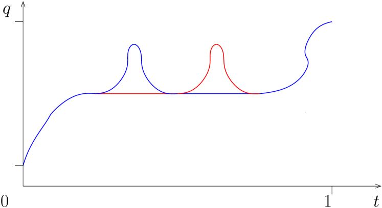
Example 10.
Let be a positive function which is constant on the interval with . Let be positive function with compact support in . Consider the family of functions given by
where is a parameter in . Then for all such , has the same end-point values, and for any smoooth functional ,
Figure 3 represents such a construction for two different values of . Note that the order of accuracy is not the issue when is smooth, as the WKB-type ansatz can be continued to obtain any order of accuracy, for a suitable . Counter examples to uniqueness such as the one depicted in Figure 3 would still hold.
The main result in this section is devoted to the extraction of a few properties of at and from moderate angles of incidence, for a sufficiently smooth .
Proposition 11.
Suppose that , and that is close to one. Using the data available for , in Problem A given by (29), the parameters given by
can be determined.
The proof of this proposition is given in section 5.
Remark 12.
This first order data respects the invariance by mirror symmetry discussed in Proposition 4. If the LC cell is flipped, its index becomes , and the parameters are unchanged. The fact that only a handful of moments can be recovered from moderate incidence is known for related more general problems, see Sharafutdinov [12].
To investigate the problem further, let us assume that the map defined in (34) is known at the endpoints and up to the order of approximation. The usable data takes the form
where , and are known parameters. Since the data is sampled in at a fine rate, the leading order dependent data is
| (36) |
which, at leading order, is given by (30). Note that this problem also arises naturally if , and not simply its amplitude, was considered in Problem A, as (36) is precisely the rate of change of the phase of .
4. On Problem B : uniqueness under a monotonicity assumption
We now turn to the reconstruction of from .
Theorem 13.
Consider for all as defined in Problem B given by (30).
-
•
The map is invariant under level-set preserving rearrangements of . That is, given two functions and defined on such that which satisfy
we have .
-
•
If is strictly increasing, , and , then determines uniquely. The reconstruction problem can be formulated in terms of classical transforms in this case. There holds
(37) where is the Laplace transform, , and is the first Hankel transform, , where is the Bessel function of the first kind of order , and is given by
Remark 14.
The Hankel Transform is self-invertible, and stable. Inverting the Laplace transform is well known to be an exponentially ill-posed task see e.g. Epstein & Schotland [13]. Even more so when, as it is the case here, the Laplace data is limited to an interval located away from zero. The data can be written as a linear integral operator acting on in the form
It is clear that is a compact operator : its inverse is therefore unbounded. Including grazing angles measures, corresponding to would still lead to an unstable problem.
To prove this result, we note that the available data takes a much simpler form after an integral transformation.
Lemma 15.
Given a function such that defined on such that , we can define as the complex valued holomorphic extension of on the annulus .
Let represent the holomorphic extension of
to the same annulus.
Let be given by
Then, for any and , we have
The correspondence between and is one to one.
We prove this result in section 5. This in turn shows that determines uniquely within the class of smooth monotone functions, albeit in a very unstable manner.
Proof of theorem 13.
The first statement is a straightforward consequence of the coarea formula applied to the map . The second statement follows from the change of variable formula as follows
Thus is the Fourier transform of on the range of . Applying the inverse Fourier transform we therefore recover the values of , and , and therefore . We do not claim that the requirement is sharp.
Let us now turn to the equation satisfied by . We write,
Using the same change of variable as above, it follows that
as announced. ∎
5. Proofs for Proposition 7, Proposition 11 and Lemma 15
We start by expressing the available data in terms of the fundamental solutions of the ordinary differential system (29). Let and be the two solution of
| (38) | |||||
We have the following identity
Proposition 16.
This is a simple calculation performed in B.
Proof of Proposition 7.
We introduce a perturbed problem closely related to the original problem when is smooth. We note given by (34) is well defined and bounded provided is small enough, namely when is bounded below by a positive constant. Assume that , with chosen so that is bounded. A tedious but straightforward computation shows that and are solutions of
| (39) | |||||
with
| (40) |
where depends on . Introducing the function given by
we find, comparing (38) and (39) and using Duhamel’s Formula, that for and there holds
And from the bound (40) we deduce that
Proposition 16 then shows that
and since , this approximation also gives an approximation for of the same order, which is the precision up to which is known. This in turn leads to the formula for announced in Proposition 7. ∎
To prove proposition 11, we focus on what can be recovered from around the normal incidence.
Proposition 17.
Suppose that , and is close to one. Then, the parameters given by
can be extracted from the data in this moderate range of incidences.
Proof.
A Taylor expansion of given (33) around , using the fact that shows that
where
Using the formula for given by (34) we find that for , for a given , we have
Without changing the order of approximation, since and are known parameters, the available data thus becomes
The conclusion follows, as we have data points available for . We could recover these five parameters either by a least square fit, or by deriving explicit formulas. ∎
Finally, we prove lemma 15.
Proof of lemma 15.
Since for every , we can write using the binomial formula
Introducing the holomorphic function of the complex variable on the annulus given by
we observe that this quantity is well defined, as the series is absolutely convergent for . As varies in , determines on a non-empty real interval and therefore also on the full annulus. We may therefore define as the holomorphic extension of .
We compute, using the residue formula on the ring of radius , that for any ,
This in turn shows, using the fact that all sums are well behaved, that
where
It turns out that has a closed form expression on the positive real line, in terms of the Error Function. For any ,
The converse transformation, using the same steps backwards, gives in terms of . ∎
6. Conclusion
We have analyzed the polarimetric measurement with variable incident angle experiment described in Lionheart & Newton [1]. After a detailed inspection of the various scales involved in the problem, we produced two related one-dimensional reconstruction problems, Problem A given by (29) and Problem B given by (30). We argued that these problems are relevant for the two Liquid Crystal Cell configurations we considered, orthorhombic and nematic uniaxial. Both problems have a simple formulation, and can be studied by applied analysts with no prior exposure to Liquid Crystals.
We partially addressed Problem A, under a smoothness assumption. Further investigation of this problem would be of practical and theoretical interest. In the smooth case, it would be interesting to see how the boundary data can be recovered in an optimal manner numerically. The non-smooth case is left open. While we do not believe that much more can be done with very general parameters, it is very possible the ill-posedness of this problem is dramatically reduced when additional constraints are imposed, e.g. when the medium is piecewise linear.
We addressed Problem B, by characterising a class of equivalent parameters, and by providing a uniqueness result when the coefficient is strictly increasing and . In that case, we show that the reconstruction amounts to of the inversion of the Laplace Transform of the Hankel Transform of a target function. We have not attempted to address the numerical resolution of such a notoriously ill-posed problem: it is very possible that it is manageable when restricted to a particular class of functions.
Acknowledgements
The authors were supported by EPSRC Science and Innovation award to the Oxford Centre for Nonlinear PDE (EP/E035027/1). The second author was also supported by EPSRC Grant EP/E010288/1 and by NSFC grant 11261054.
References
- [1] W.R.B Lionheart and C.J.P Newton. Analysis of the inverse problem for determining nematic liquid crystal director profiles from optical measurements using singular value decomposition. New Journal of Physics, 9:63, 2007.
- [2] D.W. Berreman. Optics in stratified and anisotropic media: 44-matrix formulation. JOSA, 62(4):502–510, 1972.
- [3] B. Tsering Xiao. Electromagnetic inverse problems for nematic liquid crystals. PhD thesis, 2011.
- [4] Oleg D. Lavrentovich. Looking at the world through liquid crystal glasses. In Multi-scale and high-contrast PDE: from modelling, to mathematical analysis, to inversion, volume 577 of Contemp. Math., pages 25–46. Amer. Math. Soc., Providence, RI, 2012.
- [5] M. J. Freiser. Ordered states of a nematic liquid. Phys. Rev. Lett., 24:1041–1043, 1970.
- [6] T. Hegmann, J. Kain, S. Diele, G. Pelzl, and C. Tschierske. Evidence for the existence of the mcmillan phase in a binary system of a metallomesogen and 2,4,7-trinitrofluorenone. Angew. Chem., Int. Ed., 40(5):887–890, 2001.
- [7] K. Kaznacheev and T. Hegmann. Molecular ordering in a biaxial smectic-a phase studied by scanning transmission x-ray microscopy (stxm). Phys. Chem. Chem. Phys., 9:1705–1712, 2007.
- [8] P.K. Karahaliou, A.G. Vanakaras, and D.J. Photinos. Symmetries and alignment of biaxial nematic liquid crystals. J. Chem. Phys., 131:124516, 2009.
- [9] E.G. Virga. Variational theories for liquid crystals. Chapman Hall/CRC, 1994.
- [10] P.G. de Gennes and J. Prost. The physics of liquid crystals. Oxford University Press, 1995.
- [11] S. Chandrasekhar. Liquid Crystals second edition. Cambridge University Press, UK, 1992.
- [12] V. A. Sharafutdinov. Linearized inverse problems of determining the parameters of transversally isotropic elastic media from measurements of refracted waves. J. Inverse Ill-Posed Probl., 4(3):245–266, 1996.
- [13] Charles L. Epstein and John Schotland. The bad truth about Laplace’s transform. SIAM Rev., 50(3):504–520, 2008.
- [14] Alexei D. Kiselev. Singularities in polarization resolved angular patterns: transmittance of nematic liquid crystal cells. J. Phys.: Condens. Matter, 19(24), JUN 20 2007.
- [15] Vladimir I. Arnold. Ordinary differential equations. Springer Textbook. Springer-Verlag, Berlin, 1992. Translated from the third Russian edition by Roger Cooke.
Appendix A Proof of Proposition 2
Proof.
We compute that
and since , we obtain that does not depend on . ∎
We now prove Proposition 2.
Proof of Proposition 2.
Since the entries of the matrix is are piecewise continuous functions, global existence and uniqueness of the fundamental solution of the system is well-known see e.g. [15]. Now we prove the existence and uniqueness of solutions to the transmission problem via the fundamental solution. Let us define the fundamental solution of equation (7) as follows
where
, with
We have therefore
| (41) |
where
and
To establish the announced existence and uniqueness property, let us now show that for any , . Let and be given by and .
Then the determinant of satisfies
Set and . We compute that
From the identity , we deduce that , Since and are two solutions of (7), Proposition 18 shows that this implies for all . Expressing this identity in terms of the components of and , we obtain
and in turn
| (42) |
Cauchy-Schwarz inequality thus shows that
with and . Similarly, starting from the identity and we obtain and . Therefore
∎
Appendix B Proof of Proposition 16 and Proposition 4
Problem 29 can be formulated slightly more generally as follows. Given an initial condition
find , such that , when and satisfy
with and two positive functions, bounded above and below by positive constants. This applies to system (15) with , , , and . Note is a solution of the real valued elliptic equations
| (44) |
The general uniqueness results for ordinary differential equations show that is a linear combination of the two fundamental solutions and , of (44) corresponding to the initial conditions and .
Note that the Wronskian of the problem is constant:
Using the initial and final conditions, we obtain
which leads to the following formulae for and ,
where for . Using the Wronskian identity, we note that is always well defined, as a simple calculation shows that
One can check that , therefore the amplitude of the reflected field, if it was available, would be redundant.
To prove that is unchanged if and are replaced by and , note the solution corresponding to and can be written as linear combination of and . The associated reflection and transmission coefficients and satisfy
which shows that and .