Robust price bounds for the forward starting straddle

Abstract

In this article we consider the problem of giving a robust, model-independent, lower bound on the price of a forward starting straddle with payoff $|F_{T_{1}}-F_{T_{0}}|$ where $0<T_{0}<T_{1}$. Rather than assuming a model for the underlying forward price $(F_{t})_{t\geq 0}$, we assume that call prices for maturities $T_{0}<T_{1}$ are given and hence that the marginal laws of the underlying are known. The primal problem is to find the model which is consistent with the observed call prices, and for which the price of the forward starting straddle is minimised. The dual problem is to find the cheapest semi-static subhedge.

Under an assumption on the supports of the marginal laws, but no assumption that the laws are atom-free or in any other way regular, we derive explicit expressions for the coupling which minimises the price of the option, and the form of the semi-static subhedge.

1 Introduction

We consider the problem of constructing martingales with two given marginals which minimise the expected value of the modulus of the increment. This problem has a direct correspondence to the problem in mathematical finance of giving a no-arbitrage lower bound on the price of an at-the-money forward starting straddle, given today’s vanilla call prices at the two relevant maturities. There is also a related dual problem, which is to construct the most expensive semi-static hedging strategy which sub-replicates the payoff of the forward starting straddle for any realised path of the underlying forward price process. Under a certain assumption on the distributions we solve the primal and dual problem and demonstrate that there is no duality gap.

The results of this article complement previous results by Hobson and Neuberger [20]. In that article, the authors solved the analogous problem of constructing no-arbitrage upper price bounds and semi-static super-replicating hedging strategies for the forward starting straddle. Hobson and Neuberger [20] give some examples, but the main contribution is an existence result, and a proof that the primal and dual problems yield equal values.

Returning to the lower bound case, it follows from results of Beiglböck et al [2] that there exists a solution to the primal problem and that there is no duality gap. However, Beiglböck et al [2] give an example to show that the dual supremum may not be attained. Our contribution is to show that, under a critical but natural condition on the starting and terminal law, there is an explicit construction of all the quantities of interest. (A parallel construction gives an explicit form for the optimal martingale in the upper bound setting, but in that case the condition on the measures is less natural.)

There has been a recent resurgence of interest in problems of this type, in part motivated by the connection with finance, see the survey article by Hobson [17], and in part motivated by the connections with the optimal transport problem, see [2, 3, 15]. A first strand of the mathematical finance literature is concerned with robust pricing of particular exotic derivatives, for example lookback options [16, 14], barrier options [5, 6, 9], Asian options [12], basket options [19, 10] and volatility swaps [7, 21, 18]. This strand of the literature often makes use of connections with the Skorokhod embedding problem, but in some senses the problem here is simpler in that the option payoff only depends on the joint law of $(F_{T_{0}},F_{T_{1}})$ and is otherwise path-independent. For this reason the full machinery of the Skorokhod embedding problem is not needed, although it can still help with the intuition. A second strand of the mathematical finance literature on robust pricing [8, 11, 1, 13] considers consistency between options and no-arbitrage conditions.

The optimal transport literature (see Villani [25]) is concerned with the cheapest way to transport ‘sand’ distributed according to a source measure $\mu$ to a destination measure $\nu$. Such problems are also motivated by economic questions and the transport of mass becomes an issue of the optimal allocation of economic goods. Unsurprisingly, questions of this type were of particular importance to mathematicians working on questions of efficiency in planned economies, see for instance Kantorovich [22]. The Kantorovich relaxation of Monge’s original problem goes back to his use of linear programming methods and as such, the Lagrangian approach taken in this paper is most natural. With respect to the classical optimal transport literature, the novelty of the current problem, as elucidated in Beiglböck et al [2] and developed in Beiglböck and Juillet [3] and Henry-Labordère and Touzi [15] is to add a martingale requirement to the transport plan, which is motivated by the idea that no-arbitrage considerations equate to a condition that forward prices are martingales under a pricing measure. Both [3] and [15] consider the problem of minimising the martingale transport cost for a class of cost functionals , but the payoff $|y-x|$ is not a member of this class. In contrast, here we focus exclusively on the payoff $|y-x|$. This functional encapsulates the payoff of a forward starting straddle, which is an important and simple financial product which fits into the general framework, and it is the original Monge cost function in the classical set-up. For these two reasons this cost functional is of significant interest.

2 Motivation and preliminaries

Let $X,Y$ be real-valued random variables and suppose $X\sim\mu$ and $Y\sim\nu$. We say that the bivariate law $\rho$ is a martingale coupling (equivalently a martingale transference plan) of $X$ and $Y$, and write $\rho\in{{\mathcal{M}}}(\mu,\nu)$, if $\rho$ has marginals $\mu$ and $\nu$ and is such that $\int_{y}(y-x)\rho(dx,dy)=0$ for each $x$. For a univariate measure $\zeta$ define $C_{\zeta}$ via $C_{\zeta}(x)=\int(y-x)^{+}\zeta(dy)$. It is well known (see, for instance, Strassen[24]) that ${{\mathcal{M}}}(\mu,\nu)$ is non-empty if and only if $\mu$ is less than or equal to $\nu$ in convex order, or equivalently $\mu$ and $\nu$ have equal means and $C_{\mu}(x)\leq C_{\nu}(x)$ for all $x\in{\mathbb{R}}$. Then, under the assumption that ${{\mathcal{M}}}(\mu,\nu)$ is non-empty, our goal is to find

$${{\mathcal{P}}}(\mu,\nu):=\inf_{\rho\in{{\mathcal{M}}}(\mu,\nu)}\mathop{\mathbb{E}}\nolimits[|Y-X|]\equiv\inf_{\rho\in{{\mathcal{M}}}(\mu,\nu)}\int|y-x|\rho(dx,dy).$$ (2.1)

The financial significance of this result is as follows. Let $F=(F_{t})_{t\geq 0}$ denote the forward price process of a financial asset. Let $T_{0}$ and $T_{1}$ be two future times with $0<T_{0}<T_{1}$. A well known argument due to Breeden and Litzenberger [4], shows that knowledge of a continuum of call prices for a fixed expiry is equivalent to knowledge of the marginal law at that time. Suppose then that a continuum in strike of call prices are available from a financial market and hence that it is possible to infer the marginal laws of $F$ at time $T_{0}$ and time $T_{1}$. Suppose these laws are given by $\mu$ and $\nu$. The problem is to minimise $\mathop{\mathbb{E}}\nolimits[|F_{T_{1}}-F_{T_{0}}|]$ over all martingale models for $F$ with the given marginals, i.e. to find (2.1). We will call this problem the primal problem.

Conversely, suppose we can construct a trio of functions $(\psi_{0},\psi_{1},\delta)$ such that

$$|y-x|\geq\psi_{1}(y)-\psi_{0}(x)+\delta(x)(x-y)\hskip 28.45274pt\forall x,y\in{\mathbb{R}}.$$ (2.2)

Then $\mathop{\mathbb{E}}\nolimits[|Y-X|]\geq\mathop{\mathbb{E}}\nolimits[\psi_{1}(Y)]-\mathop{\mathbb{E}}\nolimits[\psi_{0}(X)]=\int\psi_{1}(y)\nu(dy)-\int\psi_{0}(x)\mu(dx)$. It follows from (2.2) that if $\tilde{{\mathcal{S}}}$ is the set of trios of functions $(\psi_{0},\psi_{1},\delta)$ such that (2.2) holds then

$$\mathop{\mathbb{E}}\nolimits[|Y-X|]\geq\sup_{(\psi_{0},\psi_{1},\delta)\in\tilde{{\mathcal{S}}}}\left\{\int\psi_{1}(y)\nu(dy)-\int\psi_{0}(x)\mu(dx)\right\}=:{\tilde{{\mathcal{D}}}}(\mu,\nu).$$ (2.3)

We will call the problem of finding the right-hand-side of (2.3) the dual problem.

Again there is a direct financial interpretation of (2.3). Under our assumption that a continuum of calls is traded, the European contingent claims $\psi_{1}(F_{T_{1}})$ and $\psi_{0}(F_{T_{0}})$ can be replicated with portfolios of call options bought and sold at time zero. Moreover, if the agent sells forward $\delta(F_{T_{0}})$ units over $[T_{0},T_{1}]$ then the gains are $\delta(F_{T_{0}})(F_{T_{0}}-F_{T_{1}})$. Combining the two-elements of the semi-static strategy ([17, Section 2.6]) consisting of calls and a simple forward position yields

$$\psi_{1}(F_{T_{1}})-\psi_{0}(F_{T_{0}})+\delta(F_{T_{0}})(F_{T_{0}}-F_{T_{1}})$$

which corresponds to the right-hand-side of (2.2). If (2.2) holds then the semi-static strategy is a subhedge for the payoff $|F_{T_{1}}-F_{T_{0}}|$.

It is clear that if (2.2) holds then we must have $\psi_{1}(x)\leq\psi_{0}(x)$ and that if we want to find $\psi_{i}$ to maximise the right-hand-side of (2.3) then we want $\psi_{0}$ as small as possible. As a result a natural candidate for optimality is to take $\psi_{0}=\psi_{1}$ and the problem of finding a trio $(\psi_{0},\psi_{1},\delta)$ reduces to finding a pair $(\psi,\delta)$. We let ${\mathcal{S}}$ be the set of pairs $(\psi,\delta)$ such that $|y-x|\geq\psi(y)-\psi(x)+\delta(x)(y-x)$ for all $x,y$. Define

$${\mathcal{D}}(\mu,\nu)=\sup_{\psi,\delta\in{\mathcal{S}}}\left\{\int\psi(y)\nu(dy)-\int\psi(x)\mu(dx)\right\}.$$ (2.4)

Weak duality gives that ${\mathcal{P}}(\mu,\nu)\geq{\tilde{{\mathcal{D}}}}(\mu,\nu)\geq{\mathcal{D}}(\mu,\nu)$. Note that there can be no uniqueness of the dual optimiser: if $(\psi,\delta)\in{\mathcal{S}}$ then so is $(\psi+ax+b,\delta-a)$. Hence we may choose any convenient normalisation such as $\psi(x_{0})=0=\delta(x_{0})$ for some $x_{0}\in{\mathbb{R}}$.

In this article, in addition to requiring that $\mu$ and $\nu$ are increasing in convex order we will make the following additional assumption.

Dispersion Assumption 2.1.

The marginal distributions $\mu$ and $\nu$ are such that the support of $\eta:=(\mu-\nu)^{+}$ is contained in an interval $E$ and the support of $\gamma:=(\nu-\mu)^{+}$ is contained in $E^{c}$.

Weak duality gives that ${\mathcal{P}}(\mu,\nu)\geq{\tilde{{\mathcal{D}}}}(\mu,\nu)\geq{\mathcal{D}}(\mu,\nu)$. Our goal in this article is to show that ${\mathcal{P}}(\mu,\nu)={\mathcal{D}}(\mu,\nu)$ and to give explict expressions for the optimisers $\rho$, $\psi$ and $\delta$.

Remark 2.2.

Note that we make no other regularity assumptions on the measures $\mu$ and $\nu$. For example we do not require that $\mu$ and $\nu$ have densities. In contrast, Henry-Labordère and Touzi [15] assume that $\mu$ has no atoms. This is also a simplifying assumption in part of Beiglböck and Juillet [3]. Conversely, the example in Beiglböck et al [2] which shows that the dual optimiser may not exist makes essential use of the fact that $\mu$ has atoms. In our case, under Assumption 2.1 we show that a dual maximiser exists whether or not $\mu$ has atoms.

Note that if $\mu$ is less than or equal to $\nu$ in convex order and Assumption 2.1 holds then $E$ must be a finite interval. $E$ may be closed, or open, or half-open. The rationale for Assumption 2.1 will become apparent in the development of the results below. Let us, however, briefly point out that the assumption is natural in contexts most commonly encountered in mathematical finance. For instance, if the two distributions are increasing in convex order and log-normal, then Assumption 2.1 is trivially satisfied.

Example 2.3.

Let $Z$ be a random variable which is symmetric about zero and which has density $f_{Z}$ such that $zf_{Z}(z)$ is unimodal on ${\mathbb{R}}_{+}$. For $s<t$ let $X\equiv sZ$ and $Y\equiv tZ$. Let $\mu$ and $\nu$ be the laws of $X$ and $Y$. Then Assumption 2.1 holds.

2.1 Heuristics and motivation for the structure of the solution

Let $B=(B_{t})_{t\geq 0}$ be a standard Brownian motion and consider the problem of maximising or minimising $\mathop{\mathbb{E}}\nolimits[|B_{\tau}|]$ over all stopping times $\tau$, subject to the constraint that $\mathop{\mathbb{E}}\nolimits[B_{\tau}^{2}]=\mathop{\mathbb{E}}\nolimits[\tau]=1$. For the maximum, the solution is a two point distribution at $\pm 1$. This is consistent with the solution derived in Hobson and Neuberger [20] for the forward starting straddle, where in the atom-free case the solution to the problem of maximising $\mathop{\mathbb{E}}\nolimits[|Y-X|]$ subject to $X\sim\mu$, $Y\sim\nu$ and $\mathop{\mathbb{E}}\nolimits[Y|X]=X$ is characterised by a pair of increasing functions $f,g$ with $f(x)<x<g(x)$, such that, conditional on the initial value of the martingale being $x_{0}$, the terminal value of the martingale lies in $\{f(x_{0}),g(x_{0})\}$. Unfortunately, the condition that $f$ and $g$ are increasing is not sufficient to guarantee optimality and a further ‘global consistency condition’ ([20, p42]) is required.

A solution to the problem of minimising $\mathop{\mathbb{E}}\nolimits[|B_{\tau}|]$ over stopping times such that $\mathop{\mathbb{E}}\nolimits[B_{\tau}^{2}]=1$ does not exist. However, $\mathop{\mathbb{E}}\nolimits[|B_{\tau}|]$ can be made small by placing some mass at $\pm n$ and a majority of the mast at $0$. For instance, placing an atom of size $\frac{1}{2n^{2}}$ at $\pm n$ and the remaining mass $1-1/2n^{2}$ at $0$, we have $\mathop{\mathbb{E}}\nolimits[|B_{\tau}|]=1/n$. The intuition which carries over into the minimisation problem for the forward starting straddle is therefore to move as little mass as possible. In other words, we expect that subject to the same constraints as above, $\mathop{\mathbb{E}}\nolimits[|Y-X|]$ is minimised if $Y\in\{p(X),X,q(X)\}$ for functions $p,q$ with $p(x)\leq x\leq q(x)$.

2.2 Intuition for the dual problem: the Lagrangian formulation

As in [20] we take a Lagrangian approach. The problem is to minimise $\int\int|y-x|\rho(dx,dy),$ subject to the martingale and marginal conditions $\int_{x}\rho(dx,dy)=\nu(dy)$, $\int_{y}\rho(dx,dy)=\mu(dx)$, and $\int_{y}(x-y)\rho(dx,dy)=0$.

Letting $\alpha(y)$, $\beta(x)$ and $\theta(x)$ denote the multipliers for these constraints, define the Lagrangian objective function $L(x,y)=|y-x|-\alpha(y)-\beta(x)-\theta(x)(x-y)$. Then the Lagrangian formulation of the primal problem is to minimise over all measures $\rho$ on ${\mathbb{R}}^{2}$,

$$\int\int\rho(dx,dy)L(x,y)+\int\alpha(y)\nu(dy)+\int\beta(x)\nu(dx).$$ (2.5)

For a finite optimum we require $L(x,y)\geq 0$ and we expect that $L(x,y)=0$ for $y\in\{p(x),x,q(x)\}$, for a pair of functions $(p,q)$, to be determined, see Figure 1. In particular, since $L(x,x)=0$, we expect that $\beta=-\alpha$. In this case we write $L=L^{\alpha,\theta}$ where

$$L^{\alpha,\theta}(x,y)=|y-x|-\alpha(y)+\alpha(x)-\theta(x)(x-y)$$ (2.6)

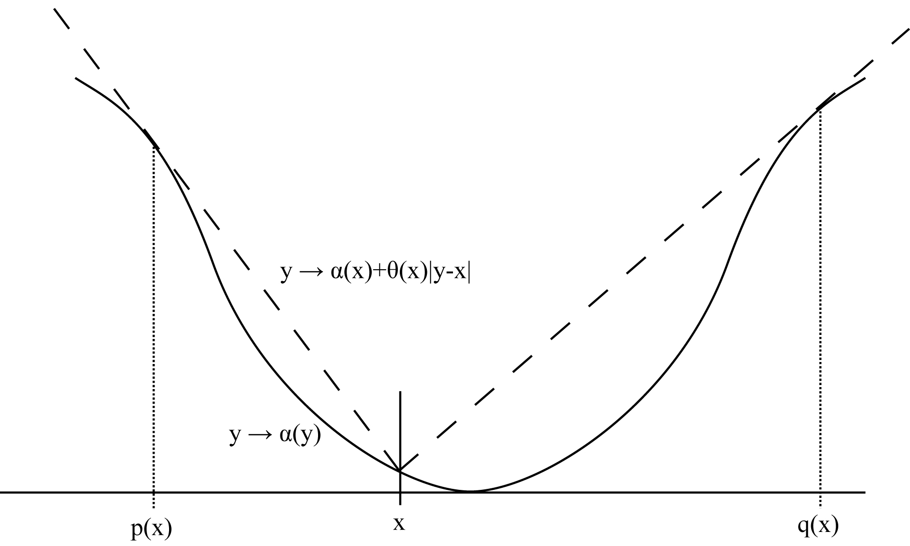
Figure 1: We have that $\alpha(x)+\theta(x)|y-x|\geq\alpha(y)$ with equality for $y\in\{p(x),x,q(x)\}$.

Assuming that $\alpha$, $\theta$, $p$ and $q$ are suitably differentiable we can derive expressions for $\alpha$ and $\theta$. The conditions $L(x,p(x))=0$, $L_{y}(x,p(x))=0$, $L(x,q(x))=0$ and $L_{y}(x,q(x))=0$ lead directly to the following equations for $x\in E$:

$$x-p(x)+\alpha(x)-\alpha(p(x))-\theta(x)(x-p(x)) = 0$$ (2.7)

$$-1-\alpha^{\prime}(p(x))+\theta(x) = 0$$ (2.8)

$$q(x)-x+\alpha(x)-\alpha(q(x))-\theta(x)(x-q(x)) = 0$$ (2.9)

$$1-\alpha^{\prime}(q(x))+\theta(x) = 0$$ (2.10)

Differentiating (2.7) and using (2.8), we obtain

$$1+\alpha^{\prime}(x)-\theta(x)-\theta^{\prime}(x)(x-p(x))=0.$$ (2.11)

Similarly, using (2.9) and (2.10), we obtain

$$-1+\alpha^{\prime}(x)-\theta(x)-\theta^{\prime}(x)(x-q(x))=0.$$ (2.12)

Subtracting the second of these two equations from the first, it follows that $\theta^{\prime}(x)=\frac{2}{q(x)-p(x)}$. Hence $\theta$ is increasing and for some $x_{0}\in E$,

$$\theta(x)=\theta(x_{0})+\int_{x_{0}}^{x}\frac{2}{q(z)-p(z)}dz.$$

Now by adding (2.11) and (2.12) we have $\alpha^{\prime}(x)=\theta(x)+\frac{\theta^{\prime}(x)}{2}(2x-p(x)-q(x))$. Then

$$\alpha(x)=x\theta(x)-\int_{x_{0}}^{x}\frac{q(z)+p(z)}{q(z)-p(z)}dz+\alpha(x_{0})-x_{0}\theta(x_{0}).$$

Moreover, from the fact that $q(x)$ is a local minimum in $y$ of $L(x,y)$ we expect $0\leq L_{yy}(x,q(x))=-\alpha^{\prime\prime}(q(x))$. Hence $\alpha$ is concave at points $y=q(x)$.

Fix $x^{\prime}<x^{\prime\prime}$. We must have that for $y\geq x^{\prime}$, $\alpha(y)\leq\alpha(x^{\prime})+(y-x^{\prime})(1+\theta(x^{\prime}))$, with equality at $y=q(x^{\prime})$. We also know that for $y\geq x^{\prime\prime}$, $\alpha(y)\leq\alpha(x^{\prime\prime})+(y-x^{\prime\prime})(1+\theta(x^{\prime\prime}))$, with equality at $y=q(x^{\prime\prime})$. Suppose that $x^{\prime\prime}\leq q(x^{\prime})$. Then

$$\alpha(x^{\prime})+(q(x^{\prime})-x^{\prime})(1+\theta(x^{\prime}))=\alpha(q(x^{\prime}))\leq\alpha(x^{\prime\prime})+(q(x^{\prime})-x^{\prime\prime})(1+\theta(x^{\prime\prime})).$$

Similarly, since $x^{\prime}<x^{\prime\prime}\leq q(x^{\prime\prime})$, we have

$$\alpha(x^{\prime\prime})+(q(x^{\prime\prime})-x^{\prime\prime})(1+\theta(x^{\prime\prime}))=\alpha(q(x^{\prime\prime}))\leq\alpha(x^{\prime})+(q(x^{\prime\prime})-x^{\prime})(1+\theta(x^{\prime})).$$

Then adding and simplifying we find $(q(x^{\prime})-q(x^{\prime\prime}))(\theta(x^{\prime\prime})-\theta(x^{\prime}))\geq 0$. But $\theta$ is increasing and thus $q(x^{\prime})\geq q(x^{\prime\prime})$. Hence $q$ is locally decreasing, in the sense that if $x^{\prime}<x^{\prime\prime}$ then either $q(x^{\prime})<x^{\prime\prime}$ or $q(x^{\prime})\geq q(x^{\prime\prime})$.

Now suppose we add Assumption 2.1. The pair $(x,q(x))$ must be such that $x\in E,q(x)\in E^{c}$. Then, if $x^{\prime}\leq x^{\prime\prime}\in E$, we cannot have $q(x^{\prime})\leq x^{\prime\prime}$. Thus $q(x^{\prime})\geq q(x^{\prime\prime})$ and $q$ is necessarily globally decreasing. Similarly $p$ is globally decreasing.

3 Determining $(p,q)$

3.1 A differential equation for $p$ and $q$.

Suppose that Assumption 2.1 is in force. Suppose that $E$ has end-points $\{a,b\}$, either of which may or may not belong to $E$. Then $p:E\mapsto(-\infty,a]$ and $q:E\mapsto[b,-\infty)$ are decreasing functions.

Recall the definitions $\eta:=(\mu-\nu)^{+}$ and $\gamma:=(\nu-\mu)^{+}$. Our martingale transport of $\mu$ to $\nu$ involves leaving common mass $(\mu\wedge\nu)$ unchanged, and otherwise mapping $\eta$ to $\gamma$.

Suppose that $\eta$ and $\gamma$ have densities $f_{\eta}$ and $f_{\gamma}$. Then we expect that $p$ and $q$ are strictly decreasing. Then $(X\neq Y,X\leq z)=(p(z)<Y\leq a)\cup(q(z)<Y)$. It follows that for $z\in E$ we have both

$$\int_{a}^{z}f_{\eta}(u)du=\int_{q(z)}^{\infty}f_{\gamma}(u)du+\int_{p(z)}^{a}f_{\gamma}(u)du,$$ (3.1)

and, from the martingale property,

$$\int_{a}^{z}uf_{\eta}(u)du=\int_{q(z)}^{\infty}uf_{\gamma}(u)du+\int_{p(z)}^{a}uf_{\gamma}(u)du.$$ (3.2)

Then by differentiating equations (3.1) and (3.2) we can derive a coupled pair of differential equations for the pair $(p,q)$:

$$p^{\prime}(x) = -\frac{q(x)-x}{q(x)-p(x)}\frac{f_{\eta}(x)}{f_{\gamma}(p(x))}\equiv\frac{q(x)-x}{q(x)-p(x)}\frac{f_{\mu}(x)-f_{\nu}(x)}{f_{\mu}(p(x))-f_{\nu}(p(x))},$$ (3.3)

$$q^{\prime}(x) = -\frac{x-p(x)}{q(x)-p(x)}\frac{f_{\eta}(x)}{f_{\gamma}(q(x))}\equiv\frac{x-p(x)}{q(x)-p(x)}\frac{f_{\mu}(x)-f_{\nu}(x)}{f_{\mu}(q(x))-f_{\nu}(q(x))}.$$ (3.4)

where $f_{\mu}$ and $f_{\nu}$ are the densities of $\mu$ and $\nu$ which we also assume to exist. Moreover we expect the boundary conditions $p(a)=\sup\{x:F_{\eta}(x)<F_{\eta}(a)\}$ and $q(a)=\sup\{x:F_{\eta}(x)<1\}$ (and similarly $p(b)=\inf\{x:F_{\eta}(x)>0\}$ and $q(b)=\inf\{x:F_{\eta}(x)>F_{\eta}(a)\}$).

Example 3.1.

Suppose $\mu\sim U[-1,1]$ and $\nu\sim U[-2,2]$. We obtain $p^{\prime}(x)=\frac{x-q(x)}{q(x)-p(x)}$ and $q^{\prime}(x)=\frac{p(x)-x}{q(x)-p(x)}$. Let $h(x)=q(x)-p(x)$ and $j(x)=q(x)+p(x)$. Note that $j^{\prime}(x)=q^{\prime}(x)+q^{\prime}(-x)=\frac{p(x)-x}{h(x)}+\frac{x-q(x)}{h(x)}=-1$. By symmetry we expect that $p(x)=-q(-x)$ and then $j(0)=0$ so that $j(x)=-x$. To derive $h$, note that $q^{\prime}(x)h(x)=p(x)-x$ and so $(h^{\prime}(x)+j^{\prime}(x))h(x)=j(x)-h(x)-2x$. Then $h^{\prime}(x)h(x)=j(x)-2x=-3x$ so that $h(x)^{2}=A-3x^{2}$ for some constant $A>0$. It follows that $q(x)=(h(x)+j(x))/2=\sqrt{q(0)^{2}-\frac{3}{4}x^{2}}-x/2$. The boundary condition $q(-1)=2$ then gives $q(0)=\sqrt{3}$ and thus $q(x)=\frac{\sqrt{12-3x^{2}}-x}{2}$. Then also a second boundary $q(1)=1$ is satisfied. Further, $p(x)=\frac{-\sqrt{12-3x^{2}}-x}{2}$.

Example 3.2.

Consider a slight modification of the above such that $\mu\sim U[-1,1]$ and $\nu\sim\frac{5}{8}U[-2,-1]+\frac{3}{8}U[1,4]$. Then, for $x\in(-1,1)$, $p^{\prime}(x)=-\frac{4}{5}\left(\frac{q(x)-x}{q(x)-p(x)}\right)$ and $q^{\prime}(x)=-4\left(\frac{x-p(x)}{q(x)-p(x)}\right)$, with boundary conditions $p(-1)=-1$ and $q(-1)=4$. This pair of coupled equations looks hard to solve. Nonetheless we will show using the methods of subsequent sections that

$$p(x)=-\frac{1}{6}\left(5+4x+\sqrt{25-8x-8x^{2}}\right);\hskip 28.45274ptq(x)=-\frac{1}{6}\left(5+4x-5\sqrt{25-8x-8x^{2}}\right).$$ (3.5)

Except when it is possible to find special simplifications it appears difficult to solve the coupled differential equations for $p$ and $q$. Indeed when the support of $\nu$ is unbounded, some care may be needed over the behaviour of $p$ and $q$ at the boundaries of $E$. More generally, if $\mu$ and $\nu$ have atoms then we cannot expect $p$ and $q$ to be differentiable, or even continuous. Instead we will take an alternative approach via the potentials of $\mu$ and $\nu$, which leads to a unique characterisation of $(p,q)$.

4 Deriving the subhedge

Motivated by the intuition of the previous section let ${\mathcal{Q}}$ be the set of pairs of decreasing functions ($p:E\mapsto(-\infty,a],q:E\mapsto[b,\infty))$. Using the monotonicity of $p$ and $q$ we can extend the domains of $p$ and $q$ to $[a,b]$. Note that we do not assume that $p$ and $q$ are differentiable or even continuous, or that they are strictly monotonic. Thus, in general $p^{-1}$ and $q^{-1}$ are set valued. Nonetheless we can define ${p_{R}^{-1}}$ and ${q_{L}^{-1}}$ to be the right-continuous and left-continuous inverses of $p$ and $q$ respectively. Then ${p_{R}^{-1}}(y)=\inf\{x\in E;p(x)\leq y\}$ with the convention that ${p_{R}^{-1}}(y)=b$ if this set is empty. Similarly ${q_{L}^{-1}}(y)=\sup\{x\in E;q(x)\geq y\}$ and ${q_{L}^{-1}}(y)=a$ if $q(a)<y$.

Definition 4.1.

Fix $x_{0}\in[a,b]$. For $(p,q)\in{\mathcal{Q}}$ define $\theta=\theta_{p,q}:[a,b]\rightarrow{\mathbb{R}}$ and $\alpha=\alpha_{p,q}:[a,b]\rightarrow{\mathbb{R}}$ via

$$\theta(x) = \int_{x_{0}}^{x}\frac{2dz}{q(z)-p(z)},$$

$$\alpha(x) = \int_{x_{0}}^{x}\frac{2x-q(z)-p(z)}{q(z)-p(z)}dz=x\theta(x)-\int_{x_{0}}^{x}\frac{q(z)+p(z)}{q(z)-p(z)}dz.$$

Extend these definitions to ${\mathbb{R}}$ by defining $\delta=\delta_{p,q}:{\mathbb{R}}\rightarrow{\mathbb{R}}$ and $\psi=\psi_{p,q}:[a,b]\rightarrow{\mathbb{R}}$ via

$$\delta(x) = \left\{\begin{array}[]{ll}\delta({p_{R}^{-1}}(x))&\;x<a,\\ \theta(x)&\;x\in[a,b],\\ \delta({p_{R}^{-1}}(x))&\;x>b.\end{array}\right.$$ (4.4)

$$\psi(x) = \left\{\begin{array}[]{ll}\alpha({p_{R}^{-1}}(x))+({p_{R}^{-1}}(x)-x)(1-\theta({p_{R}^{-1}}(x)))&\;x<a,\\ \alpha(x)&\;x\in[a,b],\\ \alpha({q_{L}^{-1}}(x))+({q_{L}^{-1}}(x)-x)(-1-\theta({q_{L}^{-1}}(x)))&\;x>b.\end{array}\right.$$ (4.8)

Lemma 4.2.

For $x>b$ (respectively $x<a$) the value of $\psi(x)$ does not depend on the choice ${q_{L}^{-1}}\in q^{-1}(x)$ (respectively ${p_{R}^{-1}}\in p^{-1}(x)$).

Proof.

Let $(z_{i})_{i=1,2}$ satisfy $q(z_{i})=x$. Then

$$\alpha(z_{2})+(z_{2}-x)(-1-\theta(z_{2}))-\{\alpha(z_{1})+(z_{1}-x)(-1-\theta(z_{1}))\}=\int_{z_{1}}^{z_{2}}\frac{2(x-q(z))}{q(z)-p(z)}dz.$$

But this expression is zero since $q(z)=x$ on $[z_{1},z_{2}]$. ∎

Example 4.3.

We calculate $\theta$ and $\alpha$ in the uniform case for which we have found $p$ and $q$ in Example 3.1. Setting $x_{0}=0$, we have

$$\theta(x)=\int_{0}^{x}\frac{2}{\sqrt{12-3u^{2}}}du=\frac{1}{\sqrt{3}}\int_{0}^{x}\frac{du}{\sqrt{1-u^{2}/4}}=\frac{2}{\sqrt{3}}\sin^{-1}\left(\frac{x}{2}\right)$$

and

$$\alpha(x)=x\theta(x)+\int_{0}^{x}\frac{udu}{\sqrt{12-3u^{2}}}=\frac{2x}{\sqrt{3}}\sin^{-1}\left(\frac{x}{2}\right)+\frac{2-\sqrt{4-x^{2}}}{\sqrt{3}}.$$

Recall the definition in (2.6) of the Lagrangian, now extended to functions $\psi$ and $\delta$ defined on ${\mathbb{R}}$,

$$L^{\psi,\delta}(x,y)=|y-x|+\psi(x)-\psi(y)+\delta(x)(y-x).$$ (4.9)

In Theorem 4.5 below we show that the Lagrangian based on (4.9) is non-negative in general and zero for $x\in\{p(x),x,q(x)\}$. It follows that the pair $(\psi,\delta)$ is a semi-static subhedge for the forward starting straddle, and hence that for any pair of random variables with $\mathop{\mathbb{E}}\nolimits[Y|X]=X$ and $X\sim\mu$, $Y\sim\nu$,

$$\mathop{\mathbb{E}}\nolimits[|Y-X|]\geq\int\psi(y)\nu(dy)-\int\psi(x)\mu(dx).$$ (4.10)

Further, given a pair of strictly monotonic functions $p:E\mapsto(-\infty,a]$ and $q:E\mapsto[b,\infty)$, a probability measure $\mu$ with density $f_{\mu}$ and a sub-probability measure $\eta\leq\mu$ with support contained in $E$ and density $f_{\eta}$, we can construct a pair $(X,\tilde{Y}=Y_{p,q,\eta,\mu})$ via $\mathop{\mathbb{P}}\nolimits(X\in dx,\tilde{Y}\in dy)=\rho^{*}(x,y)dxdy$ where

$$\rho^{*}(x,y)=\left\{\begin{array}[]{ll}f_{\eta}(x)\frac{q(x)-x}{q(x)-p(x)}I_{\{y=p(x)\}}&y<x,\\ f_{\mu}(x)-f_{\eta}(x)&y=x,\\ f_{\eta}(x)\frac{x-p(x)}{q(x)-p(x)}I_{\{y=q(x)\}}&y>x.\end{array}\right.$$

Certainly $X\sim\mu$. Let $\tilde{\nu}\equiv{\nu}_{p,q,\eta,\mu}\sim{\mathcal{L}}(\tilde{Y})$. Then $\rho^{*}(x,y)dxdy\in{\mathcal{M}}(\mu,\tilde{\nu})$ and

$$\int\int\rho^{*}(x,y)|y-x|dydx=\mathop{\mathbb{E}}\nolimits[|\tilde{Y}-X|]\geq{\mathcal{P}}(\mu,\tilde{\nu})\geq{\mathcal{D}}(\mu,\tilde{\nu})\geq\int\psi_{p,q}(y)\tilde{\nu}(dy)-\int\psi_{p,q}(x)\mu(dx)$$

and there is equality throughout, since $\rho^{*}$ is only positive when $L^{\psi_{p,q},\delta_{p,q}}=0$. In particular, ${\mathcal{P}}(\mu,\tilde{\nu})={\mathcal{D}}(\mu,\tilde{\nu})$ and there is no duality gap.

Suppose $\mu$ and $\eta$ are fixed, and consider varying $p$ and $q$. Provided it is possible to choose ${p}$ and ${q}$ such that $\tilde{\nu}\equiv{\nu}_{{p},{q},\eta,\mu}\sim\nu$ then we have

$${\mathcal{P}}(\mu,\nu)\leq\int\int\rho^{*}(x,y)|y-x|dydx=\mathop{\mathbb{E}}\nolimits[|Y-X|]=\int\psi_{{p},{q}}(y){\nu}(dy)-\int\psi_{{p},{q}}(x)\mu(dx)\leq{\mathcal{D}}(\mu,\nu).$$

Weak duality gives ${\mathcal{P}}(\mu,\nu)\geq{\mathcal{D}}(\mu,\nu)$, and hence the solutions to the primal and dual problems are the same.

Remark 4.4.

We have that for any $({p},{q})\in{\mathcal{Q}}$

$$\inf_{\rho\in{\mathcal{M}}(\mu,\nu)}\mathop{\mathbb{E}}\nolimits[|Y-X|]\geq\int\psi_{{p},{q}}(y){\nu}(dy)-\int\psi_{{p},{q}}(x)\mu(dx)$$

In financial terms this means that any $(p,q)\in{\mathcal{Q}}$ can be used to generate a semi-static subhedge $(\psi_{p,q},\delta_{p,q})$ and hence a lower bound on the price of the derivative. This bound is tight if, given $T_{0}$-call prices are consistent with $F_{T_{0}}\sim\mu$, and $T_{1}$-call prices are consistent with $F_{T_{1}}\sim\nu$, then $\nu\sim{\nu}_{p,q,\eta,\mu}$.

In the case where Assumption 2.1 holds we show in the next section how to choose functions $p$ and $q$ such that ${\nu}_{p,q,\eta,\mu}\sim\nu$ using a geometric argument. In fact, in cases where $\mu$ has atoms, generically there is no pair of functions $(p,q)$ such that $\nu_{p,q,\eta,\mu}\sim\nu$ and we have to work with multi-valued functions, or rather to re-parameterise the problem and use some independent randomisation. For the rest of this section we concentrate on showing that the choice of multipliers in Definition 4.1 leads to a non-negative Lagrangian.

Theorem 4.5.

For all $x,y\in{\mathbb{R}}$,

$$L^{\psi,\delta}=|y-x|+\psi(x)-\psi(y)-\delta(x)(x-y)\geq 0,$$

with equality for $x\in E$ and $y\in\{p(x),x,q(x)\}$.

Proof.

Suppose first that $x\in[a,b]$. If $x\leq y\leq b$, then

$$L^{\psi,\delta}(x,y) = (y-x)+x\theta(x)-\int_{x_{0}}^{x}\frac{p(z)+q(z)}{q(z)-p(z)}dz-y\theta(y)+\int_{x_{0}}^{y}\frac{p(z)+q(z)}{q(z)-p(z)}dz+\theta(x)(y-x)$$

$$= y-x+y(\theta(x)-\theta(y))+\int_{x}^{y}\frac{p(z)+q(z)}{q(z)-p(z)}dz$$

$$= \int_{x}^{y}dz\left(1-\frac{2y}{q(z)-p(z)}+\frac{p(z)+q(z)}{q(z)-p(z)}\right)$$

$$= \int_{x}^{y}dz\left(\frac{2(q(z)-y)}{q(z)-p(z)}\right)\geq 0,$$

since $q(z)\geq b\geq y$. Now for $a\leq y<x$,

$$L^{\psi,\delta}(x,y) = x-y+y(\theta(x)-\theta(y))+\int_{x}^{y}\frac{p(z)+q(z)}{q(z)-p(z)}dz$$

$$= \int_{y}^{x}dz\left(-1+\frac{2y}{q(z)-p(z)}-\frac{p(z)+q(z)}{q(z)-p(z)}\right)$$

$$= \int_{y}^{x}dz\frac{2(y-p(z))}{q(z)-p(z)}\geq 0,$$

since $p(z)\leq a\leq y$.

Next, suppose $y>b$. Let $\gamma={q_{L}^{-1}}(y)$. Then $\psi(y)=(y-\gamma)+\psi(\gamma)+\delta(\gamma)(y-\gamma)$ and $L^{\psi,\delta}(\gamma,y)=0$ by construction. It follows that

$$L^{\psi,\delta}(x,y) = (y-x)+\psi(x)-\psi(\gamma)-(y-\gamma)-\delta(\gamma)(y-\gamma)+\delta(x)(y-x)$$

$$= \alpha(x)-x\theta(x)-\alpha(\gamma)+\gamma\theta(\gamma)+\gamma-x+y(\theta(x)-\theta(\gamma))$$

$$= -\int_{x_{0}}^{x}\frac{p(z)+q(z)}{q(z)-p(z)}dz+\int_{x_{0}}^{\gamma}\frac{p(z)+q(z)}{q(z)-p(z)}dz+\int_{x}^{\gamma}dz-\int_{x}^{\gamma}\frac{2y}{q(z)-p(z)}dz$$

$$= \int_{x}^{\gamma}\frac{dz}{q(z)-p(z)}2(q(z)-y).$$

Now either $q(x)<y$ or $q(x)>y$ or $q(x)=y$. In the first case, since $q$ is decreasing, $x\geq{q_{L}^{-1}}(y)=\gamma$. Since for $z\in(\gamma,x)$, $q(z)\leq y$ we have $L^{\psi,\delta}(x,y)\geq 0$. On the other hand if $q(x)>y$ then $x\leq{q_{L}^{-1}}(y)=\gamma$ and for $z\in(x,\gamma)$, $q(z)\geq y$ and again $L^{\psi,\delta}(x,y)\geq 0$. Finally if $q(x)=y$ then $x\in q^{-1}(y)$ and $q(z)=y$ on $(x,\gamma)$ so that $L^{\psi,\delta}=0$. Similar arguments apply when $y<a$.

Finally suppose $x\notin[a,b]$. We cover the case $x<a$, the case $x>b$ being similar. For $y<{p_{R}^{-1}}(x)$,

$$0\leq L^{\psi,\delta}({p_{R}^{-1}}(x),y)=\psi({p_{R}^{-1}}(x))-\psi(y)+{p_{R}^{-1}}(x)-y+\theta({p_{R}^{-1}}(x))(y-{p_{R}^{-1}}(x)).$$

But also $L^{\psi,\delta}({p_{R}^{-1}}(x),x)=0$, and thus

$$\psi(x)=\psi({p_{R}^{-1}}(x))+{p_{R}^{-1}}(x)-x+\theta({p_{R}^{-1}}(x))(x-{p_{R}^{-1}}(x)).$$

Hence

$$0\leq L^{\psi,\delta}({p_{R}^{-1}}(x),y) = x-y+\psi(x)-\psi(y)-\theta({p_{R}^{-1}}(x))(x-y)$$

$$\leq |x-y|+\psi(x)-\psi(y)-\theta({p_{R}^{-1}}(x))(x-y)=L^{\psi,\delta}(x,y).$$

For $y\geq{p_{R}^{-1}}(x)$,

$$L^{\psi,\delta}(x,y)-L^{\psi,\delta}({p_{R}^{-1}}(x),y)=2({p_{R}^{-1}}(x)-x)>0,$$

and hence $L^{\psi,\delta}(x,y)>0$. ∎

Corollary 4.6.

$L^{\psi,\delta}(x,y)=0$ for all pairs $x\in(a,b)$ and $y\in[\lim_{z\downarrow x}q(z),\lim_{z\uparrow x}q(z)]$. Similarly $L^{\psi,\delta}(x,y)=0$ for $y\in[\lim_{z\downarrow x}p(z),\lim_{z\uparrow x}p(z)]$.

Proof.

Suppose that $q$ has a jump at $\hat{x}\in E$ and that $\hat{y}\in[\lim_{z\downarrow\hat{x}}q(z),\lim_{z\uparrow\hat{x}}q(z)]$. If $\hat{y}$ is such that $\hat{y}\neq q(\hat{x})$ then we can modify $q$ by defining $\hat{q}(\hat{x})=\hat{y}$ and $\hat{q}(x)=q(x)$ otherwise.

Write $\hat{\psi}=\psi_{p,\hat{q}}$ and $\hat{\delta}=\delta_{p,\hat{q}}$. Clearly, changing the definition of $q$ at the single point $\hat{x}$ makes no difference to the definitions of $\psi$ or $\delta$. Then,

$$L^{\psi,\delta}(\hat{x},\hat{y})=L^{\hat{\psi},\hat{\delta}}(\hat{x},\hat{y})=L^{\hat{\psi},\hat{\delta}}(\hat{x},q(\hat{x}))=0,$$

the last equality following from Theorem 4.5.

∎

5 The general case

The goal in this section is to show how to construct a martingale coupling, in the case where Assumption 2.1 holds. The aim is to construct appropriate generalised versions of $p$ and $q$, allowing for atoms, in such a way that if $X\sim\mu$, $Y\in\{p(X),X,q(X)\}$ and $\mathop{\mathbb{E}}\nolimits[Y|X]=X$ then $Y\sim\nu$.

Define $D(x)=C_{\nu}(x)-C_{\mu}(x)$. Then $D$ is a non-negative function such that $\lim_{|x|\rightarrow\infty}D(x)=0$ and, because of Assumption 2.1, $D$ is locally convex on $E^{c}$ and locally concave on $E$.

5.1 Case 1: $\mu\wedge\nu=0$

Suppose first that $\mu\wedge\nu=0$ so that $\eta=\mu$ and $\gamma=\nu$ are probability measures.

Note that not both $\eta$ and $\gamma$ can have atoms at $a$. Let $\gamma_{a}=\gamma((-\infty,a])\in(0,1)$. Then $\gamma_{a}=\max\{D^{\prime}(a-),D^{\prime}(a+)\}$.

Let $F_{\eta}^{-1}:[0,1]\mapsto[a,b]$ be the left continuous inverse of $\eta((-\infty,x])=\eta([a,x])$. For $u\in(0,1)$ define ${\mathcal{E}}_{u}(x)=D(F_{\eta}^{-1}(u))+(x-F_{\eta}^{-1}(u))(\gamma_{a}-u)-D(x)$ and

$$\phi(u)=\sup_{p<F_{\eta}^{-1}(u)<q}\frac{{\mathcal{E}}_{u}(q)-D(p)}{q-p}.$$

In regular cases, $\phi$ is the slope of the line of which is tangent to both $D$ on $(\infty,a]$ and ${\mathcal{E}}_{u}$ on $[b,\infty)$. Let $P(u),Q(u)$ be numbers such that $P(u)\leq a$, $Q(u)\geq b$ and

$$\phi(u)=\frac{{\mathcal{E}}_{u}(Q(u))-D(P(u))}{Q(u)-P(u)}.$$

It is clear from the construction, see also Figure 2, that $\phi$, $P$ and $Q$ are decreasing functions.

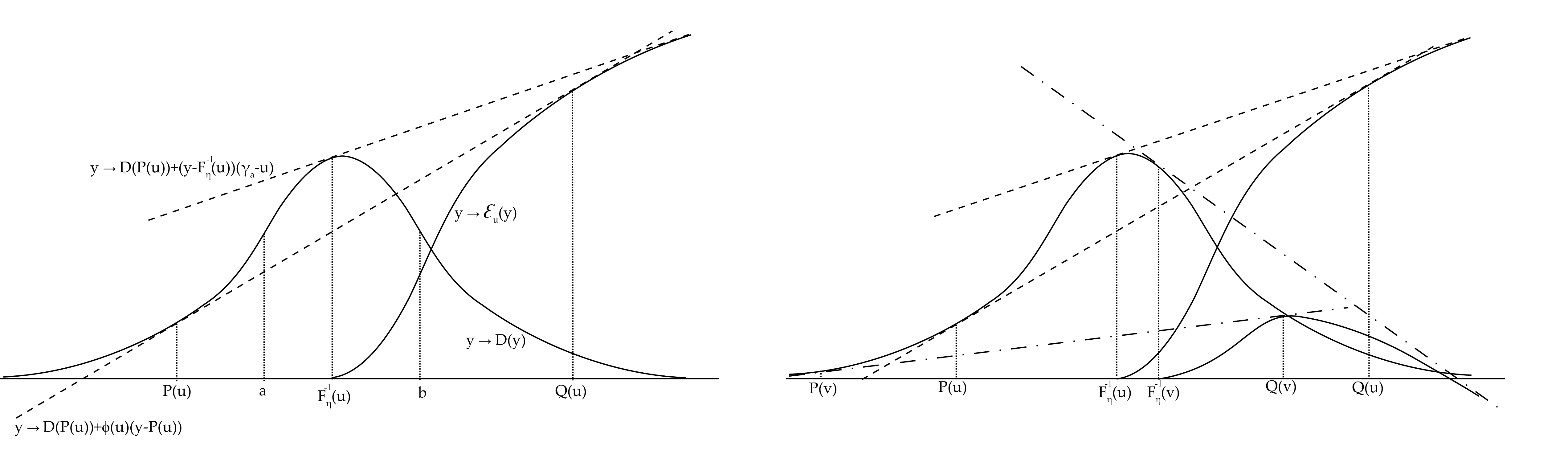
Figure 2: The left figure shows, for a single value of $u$, how $\phi(u)$ is the slope of the line which is tangent to $D(\cdot)$ at $P(u)$ and ${\mathcal{E}}_{u}(\cdot)$ at $Q(u)$. The right figure shows how as $u$ increases ${\mathcal{E}}_{u}(\cdot)$ decreases and then $P$, $Q$ and $\phi$ also all decrease.

Define

$$\zeta(u)=\inf_{p<F_{\eta}^{-1}(u)<q}\frac{D(q)-{\mathcal{E}}_{u}(p)}{q-p}\gamma_{a}-u-\phi(u).$$ (5.1)

Then $\zeta$ is the slope of the line which is tangent to both ${{\mathcal{E}}}_{u}(x)=D(F_{\eta}^{-1}(u))+(x-F_{\eta}^{-1}(u))(\gamma_{a}-u)-D(x)$, defined over $x\leq a$ and $D(x)$ defined over $x\geq b$.

Note that if $P(u)$ is unique and $D^{\prime}$ is continuous at $P(u)$ then $D^{\prime}(P(u))=\phi(u)$. Similarly, if $Q(u)$ is unique and $D^{\prime}$ is continuous at $Q(u)$ then ${\mathcal{E}}^{\prime}_{u}(Q(u))=\phi(u)$ which is equivalent to $\zeta(u)=D^{\prime}(Q(u))$. Since $\phi$ and $\zeta$ are decreasing functions and $D^{\prime}(P(u))+D^{\prime}(Q(u))=\gamma_{a}-u$, it follows that $\phi$ is Lipschitz with unit Lipschitz constant. The following lemma shows that this holds in general.

Lemma 5.1.

$\phi$ is a decreasing Lipschitz function and for $0\leq u<\hat{u}<1$, $\phi(u)\geq\phi(\hat{u})\geq\phi(u)+(u-\hat{u})$.

Proof.

It is clear that ${\mathcal{E}}_{u}(y)$ is decreasing in $u$. Then, for $\hat{u}>u$,

$$\phi(u)\geq\frac{{\mathcal{E}}_{u}(Q(\hat{u}))-D(P(\hat{u}))}{Q(\hat{u})-P(\hat{u})}>\frac{{\mathcal{E}}_{\hat{u}}(Q(\hat{u}))-D(P(\hat{u}))}{Q(\hat{u})-P(\hat{u})}=\phi(\hat{u}),$$

and hence $\phi$ is decreasing. Moreover,

$$\phi(\hat{u})\! \geq \!\frac{{\mathcal{E}}_{\hat{u}}(Q(u))-D(P(u))}{Q(u)-P(u)}$$

$$= \!\phi(u)+(u-\hat{u})\frac{Q(u)-F_{\eta}^{-1}(u)}{Q(u)-P(u)}+\frac{D(F_{\eta}^{-1}(\hat{u}))-D(F_{\eta}^{-1}(u))+(F_{\eta}^{-1}(u)-F_{\eta}^{-1})(\hat{u})(\gamma_{a}-\hat{u})}{Q(u)-P(u)}.$$

By construction the fraction in the middle term lies in $(0,1)$. Further, since $D$ is concave on $(a,b)$, $D$ lies below its tangents and the numerator in the final term is positive. Hence $\phi(\hat{u})\geq\phi(u)+u-\hat{u}$. ∎

Since $\phi$ is Lipschitz it is also absolutely continuous and we can write $\phi(u)=\gamma_{a}+\int_{0}^{u}\phi^{\prime}(w)dw$ for some function $\phi^{\prime}$.

Lemma 5.2.

We have $D(P(u))-P(u)\phi(u)=\int_{u}^{1}P(v)\phi^{\prime}(v)dv$, $D(Q(u))-Q(u)\zeta(u)=\int_{u}^{1}Q(v)\zeta^{\prime}(v)dv$ and $D(F_{\eta}^{-1}(u))-F_{\eta}^{-1}(u)(\gamma_{a}-u)=-\int_{u}^{1}F_{\eta}^{-1}(v)dv$.

Proof.

We prove the first statement, the other two being similar. Given $\{D(x);x\leq a\}$, for $\theta\in(\gamma_{a}-1,\gamma_{a})$ define the conjugate function $D_{c}(\theta)=\inf_{x\leq a}\{D(x)-\theta x\}$. Then $D_{c}(0)=0$ and $D_{c}$ is concave so that $D_{c}(\theta)=\int_{0}^{\theta}D_{c}^{\prime}(\chi)d\chi$. Note that $\phi(u)$ is an element of the subdifferential of $D$ at $P(u)$ and hence

$$D(P(u))-P(u)\phi(u)=D_{c}(\phi(u))=\int_{0}^{\phi(u)}D_{c}^{\prime}(\chi)d\chi=-\int^{1}_{u}\phi^{\prime}(v)D_{c}^{\prime}(\phi(v))dv.$$

Finally note that $D_{c}^{\prime}(\phi(v))=-(D^{\prime})^{-1}(\phi(v))=-P(v)$, almost everywhere. ∎

Note that $\phi$ has been constructed to solve

$$\phi(u)(Q(u)-P(u))=D(F_{\eta}^{-1}(u))+(Q(u)-F_{\eta}^{-1}(u))(\gamma_{a}-u)-D(Q(u))-D(P(u)).$$

Using $\phi(u)+\zeta(u)=\gamma_{a}-u$ we obtain

$$D(P(u))-P(u)\phi(u)+D(Q(u))-Q(u)\zeta(u)=D(F_{\eta}^{-1}(u))-F_{\eta}^{-1}(u)(\gamma_{a}-u)$$ (5.2)

and hence

$$\int_{u}^{1}P(v)\phi^{\prime}(v)dv+\int_{u}^{1}Q(v)\zeta^{\prime}(v)dv=-\int_{u}^{1}F_{\eta}^{-1}(v)dv.$$

Then we have both $\phi^{\prime}(u)+\zeta^{\prime}(u)=-1$ and $P(u)\phi^{\prime}(u)+Q(u)\zeta^{\prime}(u)=-F_{\eta}^{-1}(v)$ Lebesgue almost everywhere on $(0,1)$. Hence

$$\phi^{\prime}(u)=-\frac{Q(u)-F_{\eta}^{-1}(u)}{Q(u)-P(u)}\hskip 28.45274pt\mbox{almost everywhere.}$$

Theorem 5.3.

Let $U$ and $V$ be independent uniform random variables. Let $X=F_{\eta}^{-1}(U)$ and $Y=P(U)I_{A_{(U,V)}}+Q(U)I_{A^{C}_{(U,V)}}$ where

$$A_{(u,v)}=\left\{v\leq\frac{Q(u)-F_{\eta}^{-1}(u)}{(Q(u)-P(u))}\right\}.$$

Then $X$ has law $\eta$ and $Y$ has law $\gamma$.

Proof.

It is immediate that $X\sim\eta$. For $y\leq a$ let $P_{R}^{-1}=\inf\{u\in(0,1):P(u)\leq y\}$. Then

$$\mathop{\mathbb{P}}\nolimits(Y\leq y) = \int_{P_{R}^{-1}(y)}^{1}\frac{Q(u)-F_{\eta}^{-1}(u)}{Q(u)-P(u)}du$$

$$= -\int_{P_{R}^{-1}(y)}^{1}\phi^{\prime}(u)du=\phi(P_{R}^{-1}(y))=D^{\prime}(y+)=\gamma((-\infty,y]).$$

A similar argument for $y>b$ gives that $Y\sim\gamma$. ∎

5.2 Case 2: $\mu\wedge\nu\neq 0$

If $(\mu\wedge\nu)({\mathbb{R}})=1$ then we must have $Y=X$ and $\mathop{\mathbb{E}}\nolimits|Y-X|=0$. Otherwise, let $(\mu\wedge\nu)({\mathbb{R}})=\kappa\in(0,1)$. Then $\eta({\mathbb{R}})=\eta(E)=1-\kappa=\gamma(E^{c})=\gamma({\mathbb{R}})$. Define probability measures $\overline{\mu\wedge\nu}$, $\overline{\eta}$ and $\overline{\gamma}$ by $\overline{\mu\wedge\nu}(A)=(\mu\wedge\nu)(A)/\kappa$, $\overline{\eta}(A)=\eta(A)/(1-\kappa)$ and $\overline{\gamma}(A)=\gamma(A)/(1-\kappa)$.

The following result follows immediately from Theorem 5.3.

Theorem 5.4.

Let $U$ and $V$ be independent uniform random variables. and let $Z$ be a Bernoulli random variable with parameter $\kappa$. Conditional on $Z=1$, then set $Y=X\sim\overline{\mu\wedge\nu}$. Otherwise, conditional $Z=0$, let $X=F_{\overline{\eta}}^{-1}(U)$ and $Y=P(U)I_{A_{(U,V)}}+Q(U)I_{A^{C}_{(U,V)}}$ where

$$A_{(u,v)}=\left\{v\leq\frac{Q(u)-F_{\overline{eta}}^{-1}(u)}{(Q(u)-P(u))}\right\},$$

where $P$ and $Q$ are defined as in Section 5.1 for the disjoint measures $\overline{\eta}$ and $\overline{\gamma}$.

Then $X$ has law $\mu$ and $Y$ has law $\nu$.

5.3 Strong duality

Theorem 5.5.

Suppose $\mu\leq\nu$ in convex order and Assumption 2.1 holds. Then ${\mathcal{P}}(\mu,\nu)=\tilde{{\mathcal{D}}}(\mu,\nu)={\mathcal{D}}(\mu,\nu)$. Moreover, the optimal coupling is given by the construction in Theorem 5.4 and the optimal semi-static hedging strategy is given by the expressions in (4.4) and (4.8), for $(p(x),q(x))=(P(F_{\overline{\eta}}(x)),Q(F_{\overline{\eta}}(x)))$.

Proof.

By Theorems 5.3 and 5.4, we have a candidate coupling. Moreover, by Theorem 4.5 and Corollary 4.6, it follows that $L^{\psi,\delta}=0$ wherever the candidate coupling places mass, and hence, for this choice of joint law for $(X,Y)$ and $(\psi,\delta)=(\psi_{p,q},\delta_{p,q})$ we have $\mathop{\mathbb{E}}\nolimits[|Y-X|]=\int\psi(y)\nu(dy)-\int\psi(x)\mu(dx)$. Then ${\mathcal{P}}(\mu,\nu)\leq\mathop{\mathbb{E}}\nolimits[|Y-X|]=\int\psi(y)\nu(dy)-\int\psi(x)\mu(dx)\leq{\mathcal{D}}(\mu,\nu)$ and by weak duality there is equality throughout. ∎

6 Examples

6.1 The case with densities

If $\mu$ and $\nu$ have densities then it is not necessary to introduce $P$ and $Q$ and instead we can use the functions $p(x)=P(F_{\eta}(x))$ and $q(x)=Q(F_{\eta}(x))$. Then from (5.1) and (5.2) we find that the pair $(p,q)$ are characterised by

$$D^{\prime}(x) = D^{\prime}(q(x))+D^{\prime}(p(x)),$$ (6.1)

$$D(x)-xD^{\prime}(x) = D(q(x))-q(x)D^{\prime}(q(x))+D(p(x))-p(x)D^{\prime}(p(x)),$$ (6.2)

for $x\in E$.

Example 6.1.

Recall Example 3.1 and suppose $\mu\sim U[-1,1]$ and $\nu\sim U[-2,2]$.

$$D(x)=\left\{\begin{array}[]{ll}\frac{1}{8}x^{2}+\frac{1}{2}x+\frac{1}{2}&\;-2\leq x\leq-1,\\ \frac{1}{4}-\frac{1}{8}x^{2}&\;-1<x<1,\\ \frac{1}{8}x^{2}-\frac{1}{2}x+\frac{1}{2}&\;1\leq x\leq 2.\end{array}\right.$$

By (6.1), for $-1<x<1$ we have $-x=q(x)+p(x)$. Then, by (6.2) for $x\in[-1,1]$ we have

$$D(x)-xD^{\prime}(x)=D(q(x))-q(x)D^{\prime}(q(x))+D(-x-q(x))+(x+q(x))D^{\prime}(-x-q(x)).$$

After some simplification we find $q(x)^{2}+q(x)x+x^{2}-3=0$, whence $q(x)=\frac{-x+\sqrt{12-3x^{2}}}{2}$, and $p(x)=\frac{-x-\sqrt{12-3x^{2}}}{2}$.

Example 6.2.

Recall Example 3.2 and suppose that $\mu\sim U[-1,1]$ and $\nu\sim\frac{5}{8}U[-2,-1]+\frac{3}{8}U[1,4]$. Then,

$$D(x)=\left\{\begin{array}[]{ll}\frac{5}{16}(x+2)^{2}&-2\leq x\leq-1;\\ \frac{11}{16}+\frac{1}{8}x-\frac{1}{4}x^{2}&-1<x\leq 1;\\ \frac{1}{16}(4-x)^{2}&1<x\leq 4,\end{array}\right.$$

with $D\equiv 0$ outside $[-2,4]$.

Then (6.1) and (6.2) yield

$$4x+5p+q+5=0,\hskip 28.45274pt4x^{2}+5p^{2}+q^{2}=25.$$

Eliminating $q$ and solving for $p$ gives the first expression in (3.5), from which the second follows.

6.2 The general case with atoms

The full power of the analysis is illustrated in the case where $\mu$ has atoms or $\nu$ has intervals with no mass. Then there is no hope of constructing the optimal martingales via an approach using differential equations.

Example 6.3.

Let $\mu$ be any measure supported on $E=[-1,1]$ and suppose $\nu$ has support $E^{c}$ and density $\nu(dx)=|x|^{-3}dx$ for $|x|>1$. Then for $|y|>1$, $D(y)=\frac{1}{2|y|}$, $D^{\prime}(y)=-\frac{1}{2y|y|}$ and $D(y)-yD^{\prime}(y)=\frac{1}{|y|}$. Further, $\gamma_{a}=\frac{1}{2}$.

Since $\mu$ is not yet specified we do not have an expression for $D$ on $E$. Nonetheless, for $\theta\in(-\frac{1}{2},\frac{1}{2})$ we can define the conjugate $D_{c}(\theta)=\sup_{-1<x<1}(D(x)-x\theta)$, so that $D_{c}(\frac{1}{2}-u)=D(F_{\mu}^{-1}(u))-F_{\mu}^{-1}(u)(\frac{1}{2}-u)$.

Then $P=P(u)$ and $Q=Q(u)$ solve

$$\phi(u)=D^{\prime}(P)={\mathcal{E}}^{\prime}_{u}(Q)=\frac{{\mathcal{E}}_{u}(Q)-D(P)}{Q-P}$$

and hence

$$\frac{1}{2P^{2}}=\left(\frac{1}{2}-u\right)+\frac{1}{2Q^{2}}=\frac{D_{c}(\frac{1}{2}-u)+(\frac{1}{2}-u)Q-D(Q)-D(P)}{Q-P}.$$

Then, from the first equality

$$\frac{1}{P^{2}}-\frac{1}{Q^{2}}=1-2u$$ (6.3)

and

$$Q\left(\frac{1}{2}-u+\frac{1}{2Q^{2}}\right)-P\frac{1}{2P^{2}}=D_{c}\left(\frac{1}{2}-u\right)+\left(\frac{1}{2}-u\right)Q-\frac{1}{2Q}+\frac{1}{2P},$$

which simplifies to

$$\frac{1}{|P|}+\frac{1}{Q}=D_{c}\left(\frac{1}{2}-u\right).$$ (6.4)

It is straightforward to solve (6.3) and (6.4) for $1/P$ and $1/Q$ and we find

$$P(u)=-\frac{2D_{c}(\frac{1}{2}-u)}{D_{c}(\frac{1}{2}-u)^{2}+2(\frac{1}{2}-u)}\hskip 28.45274ptQ(u)=\frac{2D_{c}(\frac{1}{2}-u)}{D_{c}(\frac{1}{2}-u)^{2}-2(\frac{1}{2}-u)}.$$

For example, suppose $\mu\sim\frac{1}{2}\delta_{-1/2}+\frac{1}{2}U[0,1]$. Then, for $x\in(-1,-\frac{1}{2}]$ $D(x)=1+x/2$; for $x\in(-\frac{1}{2},0)$, $D(x)=3/4$; and for $x\in[0,1]$, $D(x)=(3-x^{2})/4$. Further, for $0<u\leq 1/2$,

$$P(u)=-\frac{(2-u)}{2-3u+u^{2}/4}\hskip 28.45274ptQ(u)=\frac{(2-u)}{u+u^{2}/4};$$

whereas, for $1/2<u<1$,

$$P(u)=-\frac{2(1-u+u^{2})}{2-4u+3u^{2}-2u^{3}+u^{4}}\hskip 28.45274ptQ(u)=\frac{2(1-u+u^{2})}{3u^{2}-2u^{3}+u^{4}}.$$

Example 6.4.

Suppose $\mu\sim U(-1,1)$ and $\nu\sim U\{-2,-1,3\}$. Then $D$ is zero outside $(-2,3)$ and $D(x)=\frac{x+2}{3}$ for $-2<x\leq-1$, $D(x)=\frac{3}{4}+\frac{x}{6}-\frac{x^{2}}{4}$ for $-1<x\leq 1$ and $D(x)=1-\frac{x}{3}$ for $1<x<3$.

It is clear that $q(x)=3$ and $p(x)=-1$ for $x<x^{*}$ and $p(x)=-2$ for $x>x^{*}$, where $x^{*}\in(-1,1)$ is to be found.

Then, see Figure 3, $x^{*}$ is the solution to

$$\left.\left\{D(x)+(y-x)D^{\prime}(x)-D(y)\right\}\right|_{y=3}=\left.\left\{D(-1)+(y+1)D^{\prime}(-1-)\right\}\right|_{y=3}=\frac{5}{3},$$

and we find $x^{*}=3-4\sqrt{\frac{2}{3}}$.

Figure 3: The point $x^{*}$ is such that the tangent to $D(\cdot)$ at $x^{*}$ meets the line $y=(x+2)/3$ (ie the linear extension of $y\mapsto D(y)$ taken over $(-2,-1)$) at $x$-coordinate 3. For $x>x^{*}$ the line joining $(-2,D(-2)=0)$ to $(3,{\mathcal{E}}_{F(x)}(3))$ lies below $D$ on $(-\infty,-1)$ and above ${\mathcal{E}}_{F(x)}$ on $(1,\infty)$. Hence, for $(x>x^{*})$ we have $(p(x)=-2,q(x)=3)$. For $x<x^{*}$ (not shown) the line joining $(-1,D(-1)=1/3)$ to $(3,{\mathcal{E}}_{F(x)}(3))$ lies below $D$ on $(-\infty,-1)$ and above ${\mathcal{E}}_{F(x)}$ on $(1,\infty)$. Hence, for $(x>x^{*})$ we have $(p(x)=-1,q(x)=3)$.

7 Concluding remarks

7.1 Upper bound

We show below that in the special case where i) $(\mu\wedge\nu)({\mathbb{R}})=0$, ii) $\mu$ has support on an interval $E$ and iii) $\nu$ has support in $E^{c}$, a modification of the above methods yields the martingale coupling which maximises $\mathop{\mathbb{E}}\nolimits[|Y-X|]$. Moreover, the optimal transport plan and the super-hedging strategies can also be given explicitly as for the lower bound case. Recall that Hobson and Neuberger [20] give an existence proof, and show that there is no duality gap, but do not give a general method for deriving explicit forms for the optimal coupling.

If $\mu$ is a point mass at $x$, then the problem is trivial and $\mathop{\mathbb{E}}\nolimits[|Y-x|]=\int|y-x|\nu(dy)$. Otherwise, proceeding as in Section 2.2, but noting that now we expect $L\leq 0$, $\beta(x)\geq-\alpha(x)$ and, conditional on $X=x$, mass at two points only, we can find equations for monotonic increasing functions (now labelled $g$ and $h$, instead of $p$ and $q$). Then $\alpha$ is convex at points $y=g(x)\leq x$ and $y=h(x)\geq x$. We find also that $g$ and $h$ are increasing. This general structure is evident in [20].

Now we add the following assumption:

Strengthened Dispersion Assumption 7.1.

The marginal distributions $\mu$ and $\nu$ are such that $(\mu\wedge\nu)({\mathbb{R}})=0$, the support of $\mu$ is contained in an interval $E$ and the support of $\nu$ is contained in $E^{c}$.

As before, suppose $E$ has endpoints $\{a,b\}$. Then necessarily $g:E\mapsto(-\infty,a]$ and $h:E\mapsto[b,\infty)$. In the case with densities we can write down equations similar to (3.1) and (3.2):

$$\int_{a}^{z}f_{\mu}(u)du = \int_{-\infty}^{g(z)}f_{\nu}(u)du+\int_{b}^{h(z)}f_{\nu}(u)du$$ (7.1)

$$\int_{a}^{z}uf_{\mu}(u)du = \int_{-\infty}^{g(z)}uf_{\nu}(u)du+\int_{b}^{h(z)}uf_{\nu}(u)du.$$ (7.2)

The defining equations for $g$ and $h$ become $C_{\mu}^{\prime}(x)=C_{\nu}^{\prime}(f(x))+C_{\nu}^{\prime}(g(x))-C_{\nu}^{\prime}(b)$ and

$$C_{\mu}(x)-xC_{\mu}^{\prime}(x)=C_{\nu}(f(x))-f(x)C^{\prime}_{\nu}(f(x))+C_{\nu}(g(x))-g(x)C^{\prime}_{\nu}(g(x))-[C_{\nu}(b)-bC^{\prime}_{\nu}(b)].$$

This time the equations do not simplify into expressions involving $D(x)=C_{\nu}(x)-C_{\mu}(x)$ alone.

By analogy with the lower bound case, and now allowing for measures which are not absolutely continuous, introduce for $u\in(0,1)$ and $y\geq b$,

$${\mathcal{F}}_{u}(y)=C_{\mu}(F^{-1}_{\mu}(u))+(y-F^{-1}_{\mu}(u))(u-1)+C_{\nu}(b)+(y-b)C^{\prime}_{\nu}(b)-C_{\nu}(y)$$

and define

$$\varphi(u)=\sup_{g\leq a<b\leq h}\frac{{\mathcal{F}}_{u}(h)-C_{\nu}(g)}{h-g}.$$

Then the suprema is attained at $G(u)\leq a<b\leq H(u)$ and

$$\varphi(u)=\frac{{\mathcal{F}}_{u}(H(u))-C_{\nu}(G(u))}{H(u)-G(u)}=C_{\nu}^{\prime}(G(u))={\mathcal{F}}_{u}^{\prime}(H(u))$$

assuming these last two derivatives exist.

Theorem 7.2.

Suppose Assumption 7.1 is in force.

Let $U$ and $V$ be independent uniform random variables. Let $X=F_{\mu}^{-1}(U)$ and $Y=G(U)I_{\tilde{A}_{(U,V)}}+H(U)I_{\tilde{A}^{C}_{(U,V)}}$ where

$$\tilde{A}_{(u,v)}=\left\{v\leq\frac{H(u)-F_{\mu}^{-1}(u)}{(H(u)-G(u))}\right\}.$$

Then $X$ has law $\mu$ and $Y$ has law $\nu$.

Moreover $\mathop{\mathbb{E}}\nolimits[|Y-X|]=\sup_{\rho\in{\mathcal{M}}(\mu,\nu)}\int\int|y-x|\rho(dx,dy)$.

Proof.

The proof of the first part of the theorem follows the proof of Theorem 5.3. The fact that this coupling yields the maximal value of $\int\int|y-x|\rho(dx,dy)$ follows from analogues of Theorem 4.5, Corollary 4.6 and Theorem 5.5. ∎

Example 7.3.

Suppose $\mu\sim U[-1,1]$ and $\nu\sim\frac{1}{2}U[-3,-1]+\frac{1}{2}U[1,3]$. Then $C_{\mu}(x)=(1-x)^{2}/4$ for $x\in(-1,1)$ and $C_{\mu}(x)=x^{-}=(-x)\vee 0$ otherwise. Further, $C_{\nu}(x)=\frac{(x+3)^{2}}{8}-x$ for $-3<x\leq-1$, $C_{\nu}(x)=1-\frac{x}{2}$ for $-1<x\leq 1$, $C_{\nu}(x)=\frac{(3-x)^{2}}{8}$ for $1<x\leq 3$ and $C_{\mu}(x)=x^{-}$ otherwise.

In this case $g(x)=G(F_{\mu}(x))$ and $h(x)=H(F_{\mu}(x))$ are well defined. Define $\tilde{{\mathcal{F}}}_{x}(y)={\mathcal{F}}_{F_{\mu}(x)}(y)$. Then $\tilde{{\mathcal{F}}}_{x}(y)=\frac{1}{8}\left(1-2x^{2}-2y+4xy-y^{2}\right)$ and it is easy to check that the pair $(g(x)=x-2,h(x)=x+2)$ solve

$$C_{\nu}^{\prime}(g(x))=\tilde{{\mathcal{F}}}^{\prime}_{x}(h(x))=\frac{\tilde{{\mathcal{F}}}_{x}(h(x))-C_{\nu}(g(x))}{h(x)-g(x)}$$

Hence $\sup_{\rho\in{\mathcal{M}}(\mu,\nu)}\int\int|y-x|\rho(dx,dy)$ is attained by the coupling $Y=X+\Theta$ where $\Theta$ is uniform on $\{\pm 2\}$ and is independent of $X$.

For this example there is a simple proof of optimality. Jensen’s inequality gives $\mathop{\mathbb{E}}\nolimits[(Y-X)^{2}]\geq(\mathop{\mathbb{E}}\nolimits[|Y-X|])^{2}$, and the left hand side is independent of the martingale coupling and equal to $\int y^{2}\nu(dy)-\int x^{2}\mu(dx)$. Hence for our example, $\mathop{\mathbb{E}}\nolimits[|Y-X|]\leq 2$ for any martingale coupling, and $\mathop{\mathbb{E}}\nolimits[|Y-X|]$ is easily seen to be equal to 2 for the coupling of the previous paragraph.

Remark 7.4.

Unlike in the lower bound case, it is not the case that if $(\mu\wedge\nu)({\mathbb{R}})>0$ then the optimal construction is to embed the common part of the distribution by setting $Y=X$ and then to embed the remaining part by the style of construction given in Theorem 7.2. This explains why we need the strengthened dispersion assumption.

7.2 The situation when the Dispersion Assumption does not hold

Return to the lower bound and consider the case where Assumption 2.1 fails. For simplicity we assume that $\mu$ and $\nu$ have densities. Then we expect there to be functions $p(x)<x<q(x)$ such that conditional on $X=x$, $Y\in\{p(x),x,q(x)\}$.

From the analysis of Section 3.1 we expect that if $x^{\prime}<x^{\prime\prime}$ then $p(x^{\prime\prime})\notin(p(x^{\prime}),x^{\prime})$ and $q(x^{\prime})\notin(x^{\prime\prime},q(x^{\prime\prime}))$. This condition is necessary for optimality, but not sufficient and there may be several candidate martingale couplings characterised by pairs $(p,q)$ with this property. A further condition is necessary, akin to the ‘global consistency condition’ of [20].

Figure 4: A viable pair $(p,q)$, in the relatively simple case where the set with $\mu-\nu>0$ consists of two intervals.

Example 7.5.

Suppose $\mu\sim U[-1,1]$ and $\nu\sim\frac{1}{4}U[-2,-1]+\frac{1}{2}\delta_{0}+\frac{1}{4}U[1,2]$ where $\delta_{0}$ denotes a point mass at zero. Suppose the mass on $[-1,0]$ is mapped to $[c,-1]\cup\{0\}\cup[d,2]$ where $-2<c<-1$ and $1<d<2$. Then mass and mean considerations imply $\frac{1}{2}=\frac{(-1-c)}{4}+\theta+\frac{(2-d)}{4}$ and $\frac{-1}{2}\frac{1}{2}=\frac{(-1-c)}{4}\frac{(c-1)}{2}+\frac{(2-d)}{4}\frac{(d+2)}{2}$ where $\theta$ is the mass mapped from $[-1,0]$ to zero, so $0\leq\theta\leq\frac{1}{2}$. These equations simplify to $c+d=4\theta-1$ and $c^{2}+d^{2}=7$. Then $d=\frac{(4\theta-1)}{2}+\frac{\sqrt{14-(4\theta-1)^{2}}}{2}$ and $c=\frac{(4\theta-1)}{2}-\frac{\sqrt{14-(4\theta-1)^{2}}}{2}$. In particular there is a parametric family of martingale couplings for which $p$ and $q$ have the appropriate monotonicity properties.

In this example we expect by symmetry that the optimal solution has $\theta=\frac{1}{4}$, and this can indeed be shown to be the case. In general further arguments are required.

7.3 Multi-timestep version

The analysis of the lower bound extends in a straightforward fashion to multiple time-points, provided an analogue of Assumption 2.1 holds.

Let $T_{0}=0<T_{1}<\ldots T_{n}$ be an increasing sequence of times and suppose the marginal distributions $\mu_{i}$ of a martingale $M$ are known at each time $T_{i}$. Consider the problem of giving a lower bound on $S=\mathop{\mathbb{E}}\nolimits[\sum_{j=1}^{n}|M_{T_{j}}-M_{T_{j-1}}|]$.

For the problem to be well-posed we must have that the family $(\mu_{i})$ is increasing in convex order. Let $\eta_{i}=(\mu_{i-1}-\mu_{i})^{+}$ and $\gamma_{i}=(\mu_{i}-\mu_{i-1})^{+}$. Suppose further that $\eta_{i}$ has support contained in an interval $E_{i}$ and $\gamma_{i}$ has support contained in $E_{i}^{c}$. Then the methods of the paper apply, and we get a tight lower bound on $S$ of the form $S\geq\sum_{i=1}^{n}{\mathcal{P}}(\mu_{i-1},\mu_{i})$.

7.4 Model independent bounds and mass transport

There have recently been several papers, including Beiglböck et al [2], Beiglböck and Juillet [3] and Henry-Labordère and Touzi [15] which have made connections between the problem of finding optimal model-independent hedges and the Monge-Kantorovich mass transport problem, and between the support of the extremal model and Brenier’s principle.

Beiglböck and Juillet [3] introduce a left-curtain martingale transport plan. This coupling has many desirable features, and using the methods of Henry-Labordère and Touzi [15] it is possible to calculate the form of the coupling in several examples. The motivations of Beiglböck and Juillet [3] in introducing the left-curtain coupling are at least threefold: firstly it is relatively tractable; secondly they use it to develop an analogue of Brenier’s principle; and thirdly this coupling minimises $\mathop{\mathbb{E}}\nolimits[c(X,Y)]$ for any cost functional $c(x,y)=h(y-x)$ where the third derivative of $h$ is positive. (Note that this manifestly excludes the case $h(z)=|z|$ which is the topic of our study.) This optimality result was extended by Henry-Labordère and Touzi [15] to include all functions $c$ which satisfy the Spence-Mirrlees type condition $c_{xyy}>0$. (One example which is natural in finance is the payoff $c(x,y)=-(\log y-\log x)^{2}$ which arises in variance swap payoffs, see also [18].)

In addition to the clear financial motivation in terms of forward starting straddles, the payoff $|y-x|$ is a natural object of study since it is the original Monge cost function in the classical (non-martingale) setting, see Rüschendorf [23]. In that setting the non-differentiability makes this payoff a relatively difficult functional to study.

The approach in [3] is based on a notion of cyclic monotonicity in a martingale setting. This has the advantage of providing existence results in a general setting but is typically not amenable to explicit solutions. In contrast, the Lagrangian approach employed in this article leads to tractable characterisations of the optimal coupling. A further contribution of this study is that unlike both [3] and [15] who assume that $\mu$ (at least) is atom-free, we indicate how to deal with atoms in $\mu$. We find a geometric representation for the optimal coupling, which can then be applied to arbitrary distributions. It is likely that these ideas can be applied more generally.

References

- [1] B. Acciaio, M. Beiglböck, F. Penkner, and W. Schachermayer. A model-free version of the fundamental theorem of asset pricing and the super-replication theorem. arXiv preprint arXiv:1301.5568, 2013.
- [2] M. Beiglböck, P. Henry-Labordère, and F. Penkner. Model-independent bounds for option prices: A mass transport approach. arXiv preprint arXiv:1106.5929, 2011.
- [3] M. Beiglboeck and N. Juillet. On a problem of optimal transport under marginal martingale constraints. arXiv preprint arXiv:1208.1509, 2012.
- [4] D.T. Breeden and R.H. Litzenberger. Prices of state-contingent claims implicit in option prices. J. Business, 51:621–651, 1978.
- [5] H. Brown, D.G. Hobson, and L. C. G. Rogers. The maximum maximum of a martingale constrained by an intermediate law. Probab. Theory Related Fields, 119(4):558–578, 2001.
- [6] H. Brown, D.G. Hobson, and L. C. G. Rogers. Robust hedging of barrier options. Math. Finance, 11(3):285–314, 2001.
- [7] P. Carr and R. Lee. Hedging variance options on semi-martingales. Finance and Stochastics, 14(2):179–208, 2010.
- [8] L. Cousot. Conditions on options prices for absence of arbitrage and exact calibration. Journal of banking and Finance, 31(11):3377–3397, 2007.
- [9] A. Cox and J. Wang. Root’s barrier: construction, optimality and applications to variance options. annals of Applied Probability, 23(3):859–894, 2013.
- [10] A. d’Aspremont and L. El Ghaoui. Static arbitrage bounds on basket option prices. Mathematical Programming, Series A, 106(3):467–489, 2006.
- [11] M.H.A. Davis and D.G. Hobson. The range of traded option prices. Mathematical Finance, 17(1):1–14, 2007.
- [12] J. Dhaene, M. Denuit, M.J. Goovaerts, R. Kaas, and D. Vyncke. The concept of co-monotonicity in actuarial science and finance: applications. Insurance: Mathematics and Economics, 31:133–161, 2002.
- [13] Y. Dolinsky and H.M. Soner. Martingale optimal transport and robust hedging in continuous time. arXiv:1208.4922, 2013.
- [14] A. Galichon, P. Henry-Labordere, and N. Touzi. A stochastic control approach to no-arbitrage bounds with given marginals, with an application to lookback options. Annals of Applied Probability, to appear, 2013.
- [15] P. Henry-Labordere and N. Touzi. An explicit martingale version of brenier’s theorem. arXiv preprint arXiv:1302.4854, 2013.
- [16] D.G Hobson. Robust hedging of the lookback option. Finance and Stochastics, 2:329–347, 1998.
- [17] D.G. Hobson. The Skorokhod embedding problem and model independent bounds for option prices. In Paris-Princeton Lecture Notes on Mathematical Finance. Springer, 2010.
- [18] D.G. Hobson and M. Klimmek. Model-independent hedging strategies for variance swaps. Finance and Stochastics, 16(4):611–649, 2012.
- [19] D.G. Hobson, P. Laurence, and T-H. Wang. Static-arbitrage upper bounds for the prices of basket options. Quantitative Finance, 5:329–342, 2005.
- [20] D.G. Hobson and A. Neuberger. Robust bounds for forward-start options. Mathematical Finance, 22(1):31–56, 2008.
- [21] N. Kahale. Model-independent lower bound on variance swaps. Available at SSRN 1493722, 2011.
- [22] L.V Kantorovich. Lecture to the memory of Alfred Nobel: Mathematics in Economics: Achievements, difficulties, perspectives. www.nobelprize.org/nobel_prizes/economics/laureates/1975/kantorovich-lecture.html, 1975.
- [23] L. Rüschendorf. Monge-Kantorovich transportation problem and optimal couplings. Jahresbericht der DMV, 109:113–137, 2007.
- [24] V. Strassen. Almost sure behavior of sums of independent random variables and martingales. In Proc. Fifth Berkeley Sympos. Math. Statist. and Probability (Berkeley, Calif., 1965/66), pages Vol. II: Contributions to Probability Theory, Part 1, pp. 315–343. Univ. California Press, Berkeley, Calif., 1967.
- [25] C. Villani. Optimal Transport: Old and New. Springer-Verlag, 2009.