HATS-2b: A transiting extrasolar planet orbiting a K-type star showing starspot activity

We report the discovery of HATS-2b, the second transiting extrasolar planet detected by the HATSouth survey. HATS-2b is moving on a circular orbit around a $V=13.6$ mag, K-type dwarf star (GSC 6665-00236), at a separation of $0.0230\pm 0.0003$ AU and with a period of $1.3541$ days. The planetary parameters have been robustly determined using a simultaneous fit of the HATSouth, MPG/ESO 2.2 m/GROND, Faulkes Telescope South/Spectral transit photometry and MPG/ESO 2.2 m/FEROS, Euler 1.2 m/CORALIE, AAT 3.9 m/CYCLOPS radial-velocity measurements. HATS-2b has a mass of $1.37\pm 0.16$ $M_{J}$, a radius of $1.14\pm 0.03$ $R_{J}$ and an equilibrium temperature of $1567\pm 30$ K. The host star has a mass of $0.88\pm 0.04$ $M_{\astrosun}$, radius of $0.89\pm 0.02$ $R_{\astrosun}$ and shows starspot activity. We characterized the stellar activity by analysing two photometric-follow-up transit light curves taken with the GROND instrument, both obtained simultaneously in four optical bands (covering the wavelength range of $3860-9520$ Å). The two light curves contain anomalies compatible with starspots on the photosphere of the host star along the same transit chord.

1 Introduction

The first detection of a planet orbiting a main-sequence star (51 Peg; Mayor & Queloz, 1995) started a new era of astronomy and planetary sciences. In the years since, the focus on exoplanetary discovery has steadily increased, resulting in more than 850 planets being detected in 677 planetary systems. Statistical implications of the exoplanet discoveries, based on different detection methods, have also been presented (e.g. Mayor et al., 2011; Howard et al., 2012; Cassan et al., 2012; Fressin et al., 2013). Most of these planets have been detected by the transit and radial velocity (RV) techniques. The former detects the decrease in a host star’s brightness due to the transit of a planet in front of it, while the latter measures the Doppler shift of host star light due to stellar motion around the star-planet barycenter. In the case of transiting extrasolar planets, the powerful combination of both methods permits a direct estimate of mass and radius of the planetary companion and therefore of the planetary average density and surface gravity. Such information is of fundamental importance in establishing the correct theoretical framework of planet formation and evolution (e.g. Liu et al., 2011; Mordasini et al., 2012a, b).

Thanks to the effectiveness of ground- and space-based transit surveys like TrES (Alonso et al., 2004), XO (McCullough et al., 2005), HATNet (e.g. Bakos et al., 2012a; Hartman et al., 2012), HATSouth (Penev et al., 2013), WASP (e.g. Hellier et al., 2012; Smalley et al., 2012), QES (Alsubai et al., 2011; Bryan et al., 2012), KELT (Siverd et al., 2012), COROT (e.g. Rouan et al., 2012; Pätzold et al., 2013) and Kepler (Borucki et al., 2011a, b; Batalha et al., 2012), one third of the transiting exoplanets known today were detected in the past 2 years. In some cases, extensive follow-up campaigns have been necessary to determine the correct physical properties of several planetary systems (e.g. Southworth et al., 2011; Barros et al., 2011; Mancini et al., 2013a), or have been used to discover other planets by measuring transit time variations (e.g. Rabus et al., 2009b, Steffen et al., 2013). With high-quality photometric observations it is also possible to detect transit anomalies which are connected with physical phenomena, such as star spots (Pont et al., 2007; Rabus et al., 2009; Désert, 2011; Tregloan-Reed et al., 2013), gravity darkening (Barnes, 2009; Szabó et al., 2011), stellar pulsations (Collier Cameron et al., 2010), tidal distortion (Li et al., 2010; Leconte et al., 2011), and the presence of additional bodies (exomoons) (Kipping et al., 2009; Tusnski & Valio, 2011).

In this paper we report the detection of HATS-2b, the second confirmed exoplanet found by the HATSouth transit survey. HATSouth is the first global network of robotic wide-field telescopes, located at three sites in the Southern hemisphere: Las Campanas Observatory (Chile), Siding Spring Observatory (Australia) and H.E.S.S. (High Energy Stereoscopic System) site (Namibia). We refer the reader to Bakos et al. (2013), where the HATSouth instruments and operations are described in detail. HATS-2b is orbiting a K-type dwarf star and has characteristics similar to those of most hot-Jupiter detected so far. Photometric follow-up performed during two transits of this planet clearly reveals anomalies in the corresponding light curves, which are very likely related to the starspot activity of the host star.

2 Observations

2.1 Photometry

The star HATS-2 (GSC 6665-00236; $V=13.562\pm 0.016$; J2000 $\alpha=11^{\mathrm{h}}46^{\mathrm{m}}57^{\mathrm{s}}.38$, $\delta=-22^{\circ}33^{\prime}46^{\prime\prime}.77$, proper motion $\mu_{\alpha}=-45.8\pm 1.1$ mas/yr, $\mu_{\delta}=-1.3\pm 1.5$ mas/yr; UCAC4 catalogue, Zacharias et al., 2012) was identified as a potential exoplanet host based on photometry from all the instruments of the HATSouth facility (HS-1 to HS-6) between Jan 19 and Aug 10, 2010 (details are reported in Table 1). The detection light curve is shown in Figure 1. This figure shows that the discovery data is of sufficient quality that it permits fitting a Mandel & Agol (2002) limb-darkened transit model. A detailed overview of the observations, the data reduction and analysis is given in Bakos et al. (2013).

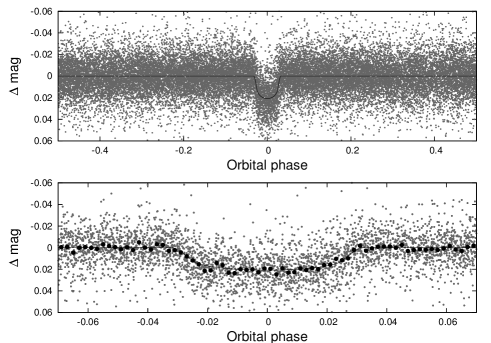
Figure 1: Top panel: Unbinned instrumental $r$-band light curve of HATS-2 folded with the period P = 1.354133 days resulting from the global fit described in Section 3. Lower panel: zoom in on the transit; the dark filled points show the light curve binned in phase using a bin size of 0.002. In both panels, the solid line shows the best-fit transit model (see Section 3.4).

HATS-2 was afterwards photometrically followed-up three times by two different instruments at two different telescopes. On UT 2011, June 25, the mid-transit and the egress were observed with the “Spectral” imaging camera, mounted at 2.0 m Faulkes Telescope South (FTS), situated at Siding Spring Observatory (SSO) and operated as part of the Las Cumbres Observatory Global Telescope (LCOGT) network. The Spectral camera hosts a 4K$\times$4K array of $0.15^{\prime\prime}$ pixels, which is readout with $2\times 2$ binning. We defocus the telescope to reduce the effect of imperfect flat-fielding and to allow for longer exposure times without saturating. We use an $i$-band filter and exposure times of 30 s, which with a 20 s readout time gives 50 s cadence photometry. The data is calibrated with the automated LCOGT reduction pipeline, which includes flat-field correction and fitting an astrometric solution. Photometry is performed on the reduced images using an automated pipeline based on aperture photometry with Source Extractor (Bertin & Arnouts, 1996). The partial transit observed is shown in Figure 2, and permitted a refinement of the transit depth and ephemeris. The latter was particularly important for the subsequent follow-up observations performed with the MPG/ESO 2.2m telescope at the La Silla Observatory (LSO). Two full transits were covered on February 28 and June 1, 2012, using GROND (Gamma-Ray Burst Optical/Near-Infrared Detector), which is an imaging camera capable of simultaneous photometric observations in four optical (identical to Sloan $g$, $r$, $i$, $z$) passbands (Greiner et al., 2008). The main characteristics of the cameras and details of the data reduction are described in Penev et al. (2013). The GROND observations were performed with the telescope defocussed and using relatively long exposure times (80-90 s, 150-200 s cadence). This way minimises noise sources (e.g. flat-fielding errors, atmospheric variation or scintillation, variation in seeing, bad tracking and Poisson noise) and delivers high-precision photometry of transit events (Alonso et al., 2008; Southworth et al., 2009). The light curves and their best-fitting models are shown in Fig. 2. Distortions in the GROND light curves are clearly visible, which we ascribe to stellar activity. These patterns are analysed in detail in Section 4. Table 1 gives an overview of all the photometric observations for HATS-2.

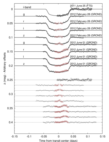
Figure 2: Phased transit light curves of HATS-2. The dates and instruments used for each event are indicated. The light curves are ordered according to the date and to the central wavelength of the filter used (Sloan $g$, $r$, $i$ and $z$). Our best fit is shown by the solid lines (see Section 3.4). Residuals from the fits are displayed at the bottom, in the same order as the top curves. The GROND datapoints affected by anomalies are marked with red empty squares and were not considered in estimating the final values of the planetary-system parameters (see Sect. 4).

Table 1: Summary of photometric observations of HATS-2

Facility	Date(s)	# of images	Cadence (s)	Filter
Discovery
HS-1 (Chile)	2010, Jan 24 - Aug 09	5913	280	Sloan $r$
HS-2 (Chile)	2010, Feb 11 - Aug 10	10195	280	Sloan $r$
HS-3 (Namibia)	2010, Feb 12 - Aug 10	1159	280	Sloan $r$
HS-4 (Namibia)	2010, Jan 26 - Aug 10	8405	280	Sloan $r$
HS-5 (Australia)	2010, Jan 19 - Aug 08	640	280	Sloan $r$
HS-6 (Australia)	2010, Aug 06	8	280	Sloan $r$
Follow-up
FTS/Spectral	2011, June 25	158	50	Sloan $i$
MPG/ESO 2.2 m / GROND	2012, February 28	69	80	Sloan $g$
MPG/ESO 2.2 m / GROND	2012, February 28	70	80	Sloan $r$
MPG/ESO 2.2 m / GROND	2012, February 28	69	80	Sloan $i$
MPG/ESO 2.2 m / GROND	2012, February 28	71	80	Sloan $z$
MPG/ESO 2.2 m / GROND	2012, June 1	99	80	Sloan $g$
MPG/ESO 2.2 m / GROND	2012, June 1	99	80	Sloan $r$
MPG/ESO 2.2 m / GROND	2012, June 1	99	80	Sloan $i$
MPG/ESO 2.2 m / GROND	2012, June 1	99	80	Sloan $z$

2.2 Spectroscopy

HATS-2 was spectroscopically followed-up between May 2011 and April 2012 by five different instruments at five individual telescopes. The follow-up observations started in May 2011 with high signal to noise (S/N) medium resolution ($\lambda/\Delta\lambda$ = 7000) reconnaissance observations performed at the ANU 2.3 m telescope located at SSO, with the image slicing integral field spectrograph WiFeS (Dopita et al., 2007). The results showed no RV variation with amplitude greater than 2 km s^-1; this excludes most false-positive scenarios involving eclipsing binaries. Furthermore, an initial determination of the stellar atmospheric parameters was possible ($T_{eff,\star}=4800\pm 300\,K$, $\log g_{\star}=4.4\pm 0.3$), indicating that HATS-2 is a dwarf star. Within the same month, high precision RV follow-up observations started with the fibre-fed echelle spectrograph CORALIE (Queloz et al., 2000b) at the Swiss Leonard Euler 1.2 m telescope at LSO, followed by further high precision RV measurements obtained with the fibre-fed optical echelle spectrograph FEROS (Kaufer & Pasquini, 1998) at the MPG/ESO 2.2 m telescope at LSO. Using the spectral synthesis code SME (‘Spectroscopy Made Easy’, Valenti & Piskunov, 1996) on the FEROS spectra, it was possible to determine more accurate values for the stellar parameters (see Sect. 3.1). Further RV measurements were obtained with the CYCLOPS fibre-based integral field unit, feeding the cross-dispersed echelle spectrograph UCLES, mounted at the 3.9 m Anglo-Australian Telescope (AAT) at SSO, and with the fibre-fed echelle spectrograph FIES at the 2.5 m telescope at the Nordic Optical Telescope in La Palma. We refer to Penev et al. (2013) for a more detailed description of the observations, the data reduction and the RV determination methods for each individual instrument that we utilized.

In total, 29 spectra were obtained, which are summarized in Table 2. Table 3 provides the high-precision RV and bisector span measurements. Figure 3 shows the combined high-precision RV measurements folded with the period of the transits. The error bars of the RV measurements include a component from astrophysical/instrumental jitter allowed to differ for the three instruments (Coralie: 74.0 ms^-1, FEROS: 44.0 ms^-1, CYCLOPS: 193.0 ms^-1, see Sec. 3.3).

Figure 3: Top panel: high-precision RV measurements for HATS-2 from CORALIE (dark filled circles), FEROS (open triangles) and CYCLOPS (filled triangles) shown as a function of orbital phase, together with our best-fit model. Zero phase corresponds to the time of mid-transit. The center-of-mass velocity has been subtracted. Second panel: velocity O-C residuals from the best fit. The error bars include a component from astrophysical/instrumental jitter allowed to differ for the three instruments (see Sec. 3.3). Third panel: bisector spans (BS), with the mean value subtracted. Note the different vertical scales of the panels.

Table 2: Summary of spectroscopic observations of HATS-2. Observing mode: HPRV = high-precision RV measurements, RECON = reconnaissance observations.

Telescope/Instrument	Date Range	# of Observations	Instrument resolution	Observing mode
ANU 2.3 m/WiFeS	2011, May 10-15	5	7000	RECON
Euler 1.2 m/Coralie	2011, May 20-21	4	60000	HPRV
ESO/MPG 2.2 m/FEROS	2011, June 09-25	9	48000	HPRV
ESO/MPG 2.2 m/FEROS	2012, January 12	1	48000	HPRV
ESO/MPG 2.2 m/FEROS	2012, March 04-06	2	48000	HPRV
ESO/MPG 2.2 m/FEROS	2012, April 14-18	3	48000	HPRV
AAT 3.9 m/CYCLOPS	2012, January 05-12	4	70000	HPRV
NOT 2.5 m/FIES	2012, March 15	1	46000	RECON

Table 3: Relative RV and bisector span (BS) measurements of HATS-2 from various instruments used for high-precision RV measurements (c.f. Table 2). 5 data points determined with FEROS are not listed here and were not used for further analysis due to high error bars caused by bad weather conditions.

BJD	Relative RV	$\sigma_{\rm{RV}}$	BS	$\sigma_{\rm{BS}}$	Phase	Exp. Time	S/N	Instrument
(-2454000)	m s-1)	(m s-1)	(m s-1)	(m s-1)		(s)
$1701.52346$	$-90.37$	$33.00$	$-63.7$	$79.5$	$0.119$	1800	9.0	Coralie
$1701.54622$	$-238.37$	$36.00$	$117.7$	$83.3$	$0.135$	1800	8.0	Coralie
$1702.52760$	$168.63$	$33.00$	$31.3$	$58.6$	$0.860$	1800	10.0	Coralie
$1702.55065$	$169.63$	$33.00$	$-30.8$	$74.2$	$0.877$	1800	9.0	Coralie
$1721.50300$	$204.15$	$71.76$	$120.4$	$93.8$	$0.873$	2400	14.0	FEROS
$1722.58300$	$371.99$	$100.77$	$-146.9$	$640.0$	$0.671$	2400	16.0	FEROS
$1723.44500$	$-330.70$	$73.66$	$-211.0$	$207.2$	$0.307$	2400	18.0	FEROS
$1736.46900$	$164.63$	$38.18$	$149.3$	$86.4$	$0.925$	2400	16.0	FEROS
$1737.53800$	$261.69$	$119.02$	$-130.9$	$287.5$	$0.715$	1044	17.0	FEROS
$1738.48600$	$-47.00$	$58.61$	$-222.1$	$146.9$	$0.415$	3000	12.0	FEROS
$1932.22448$	$-33.63$	$21.80$	$1114.3$	$43.2$	$0.487$	2400	22.7	CYCLOPS
$1933.21669$	$-40.53$	$51.20$	$3464.1$	$19.9$	$0.219$	2400	20.7	CYCLOPS
$1934.12774$	$75.57$	$65.58$	$-4516.6$	$168.1$	$0.892$	2400	17.6	CYCLOPS
$1938.81200$	$-337.82$	$139.13$	$-436.4$	$449.1$	$0.351$	2700	17.0	FEROS
$1939.16016$	$47.07$	$49.44$	$9189.5$	$1723.7$	$0.608$	2400	18.0	CYCLOPS
$1990.75600$	$294.99$	$103.71$	$46.3$	$201.6$	$0.711$	2700	15.0	FEROS
$1992.82100$	$-335.90$	$72.26$	$-251.5$	$208.5$	$0.236$	2700	19.0	FEROS
$2035.67400$	$31.55$	$77.56$	$270.6$	$223.1$	$0.882$	3600	22.0	FEROS

3 Analysis

3.1 Stellar parameters

As already mentioned in Sect. 2.2, we estimated the stellar parameters, i.e. effective temperature $T_{eff\star}$, metallicity [Fe/H], surface gravity $\log g$ and projected rotational velocity $v\sin i$, by applying SME on the high-resolution FEROS spectra. SME determines stellar and atomic parameters by fitting spectra from model atmospheres to observed spectra and estimates the parameter errors using the quality of the fit, expressed by the reduced $\chi^{2}$, as indicator. In case the S/N is not very high, or the spectrum is contaminated with telluric absorption features, cosmics or stellar emission lines, the reduced $\chi^{2}$ does not always converge to unity, which leads to small errors for the stellar parameter values. To estimate of error bars, we used SME to determine the stellar parameters of each FEROS spectrum and calculated the weighted mean and corresponding scatter (weighted by the S/N of individual spectra). The results for the spectroscopic stellar parameters including the assumed values for micro- $v_{mic}$ and macroturbulence $v_{mac}$ of the SME analysis are listed in Table 4.

By modeling the light curve alone it is possible to determine the stellar mean density, which is closely related to the normalized semimajor axis $a/R_{\star}$ (Sect. 3.4) assuming a circular orbit. Furthermore, adding RV measurements allows the determination of these parameters for elliptical orbits as well.

To obtain the light curve model, quadratic limb-darkening coefficients are needed, which were determined using Claret (2004) and the initially determined stellar spectroscopic parameters. We used the Yonsei-Yale stellar evolution models (Yi et al., 2001; hereafter YY) to determine fundamental stellar parameters such as the mass, radius, age and luminosity. The light curve based stellar mean density and spectroscopy based effective temperature and metallicity, coupled with isochrone analysis, together permit a more accurate stellar surface gravity determination. To allow uncertainties in the measured parameters to propagate into the stellar physical parameters we assign an effective temperature and metallicity, drawn from uncorrelated Gaussian distributions, to each stellar mean density in our MCMC chain, and perform the isochrone look-up for each link in the MCMC chain. The newly determined value for $\log g_{\star}=4.50\pm 0.05$ is consistent with the initial value of $\log g_{\star}=4.44\pm 0.12$ thus we refrain from re-analyzing the spectra fixing the surface gravity to the revised value.

Table 4: Stellar parameters for HATS-2

Parameter	Value	Source
Spectroscopic properties
$T_{eff\star}$ (K)	$5227\pm 95$	SME
$[Fe/H]$	$0.15\pm 0.05$	SME
$v\sin i_{\star}$ (km s-1)	$1.5\pm 0.5$	SME
$\log g_{\star}$ (cgs)	$4.44\pm 0.12$	SME
$v_{mic}$ (km s-1)a	1.5	SME
$v_{mac}$ (km s-1)a	2.0	SME
Photometric properties
$V$ (mag)	$13.562\pm 0.016$	APASS1
$B$ (mag)	$14.490\pm 0.031$	APASS
$g$ (mag)	$13.991\pm 0.012$	APASS
$r$ (mag)	$13.260\pm 0.020$	APASS
$i$ (mag)	$13.018\pm 0.021$	APASS
$J$ (mag)	$11.906\pm 0.024$	2MASS2
$H$ (mag)	$11.475\pm 0.023$	2MASS
$K$ (mag)	$11.386\pm 0.023$	2MASS
Derived properties
$M_{\star}$ ($M_{\astrosun}$)	$0.882\pm 0.037$	YY+$a/R_{\star}$+SME
$R_{\star}$ ($R_{\astrosun}$)	$0.898\pm 0.019$	YY+$a/R_{\star}$+SME
$\log g_{\star}$ (cgs)	$4.48\pm 0.02$	YY+$a/R_{\star}$+SME
$L_{\star}$ ($L_{\astrosun}$)	$0.54\pm 0.06$	YY+$a/R_{\star}$+SME
$M_{V}$ (mag)	$5.61\pm 0.13$	YY+$a/R_{\star}$+SME
$M_{K}$ (mag)	$3.64\pm 0.07$	YY+$a/R_{\star}$+SME
Age (Gyr)	$9.7\pm 2.9$	YY+$a/R_{\star}$+SME
Distance (pc)b	$360\pm 11$	YY+$a/R_{\star}$+SME
$P_{\star,\rm{rot}}$ (d)c	$30.32\pm 10.13$

The spectroscopic, photometric and derived stellar properties are listed in Table 4, whereas the adopted quadratic limb-darkening coefficients for the individual photometric filters are shown in Table 5.

To illustrate the position of HATS-2 in the H-R diagram, we plotted the normalized semi-major axis $a/R_{\star}$ versus effective temperature $T_{eff\star}$. Figure 4 shows the values for HATS-2 with their 1-$\sigma$ and 2-$\sigma$ confidence ellipsoids as well as YY-isochrones calculated for the determined metallicity of [Fe/H]$=0.15$ and interpolated to values between 1 and 14 Gyr in 1 Gyr increments from our adopted model.

Figure 4: YY-isochrones from Yi et al. (2001) for the metallicity of [Fe/H]$=0.15$. Isochrones are plotted for ages between 1 and 14 Gyr in steps of 1 Gyr (left to right). The ellipses mark the 1-$\sigma$ and 2-$\sigma$ confidence ellipsoids for the determined values of $a/R_{\star}$ and $T_{eff\star}$. The isochrones plotted here have a fixed metallicity for visualization purposes only, uncertainties on the metallicity are propagated into the uncertainties on the stellar mass and radius.

3.2 Stellar rotation

We applied the Lomb-Scargle periodogram (Lomb, 1976; Scargle, 1982) to the HATSouth light curve for HATS-2 and found a significant peak at a period of $P=12.46\pm 0.02$ d with a S/N measured in the periodogram of $87$ and a formal false alarm probability of $10^{-98}$ calculated following Press et al. (1992). Fig. 5 shows the normalized Lomb-Scargle periodogram of the HATSouth light curve. The peak-to-peak amplitude of the signal over the full 203 d spanned by the observations is 7.4 mmag. If we split the data into bins of duration 50 d, the amplitude in each bin varies from 3.6 mmag to 10.0 mmag. We interpret this signal as being due to starspots modulated by the rotation of the star. The stellar rotation period is thus $\sim 12.5$ d, or twice this value (as seen in many open clusters, an individual star often shows two minima per cycle so that the rotation period is double the value found from a periodogram analysis; also note that due to differential rotation and the unknown latitudinal distribution of spots on the star, the equatorial period may be as much as 10–20% shorter than the measured period). Both rotation periods (12.5 and 25 d) are consistent with the upper limit of $P_{\star,\rm{rot}}$ of $30.32\pm 10.13\,$d derived from the determined $v\sin i$ and $R_{\star}$ (see Tab. 4). The rotation period of $12.46$ d is comparable to that of similar-size stars in the 1 Gyr open cluster NGC 6811 (Meibom et al., 2011), which shows a tight period–color sequence. The spin-down rate for sub-solar-mass stars is poorly constrained beyond 1 Gyr, but assuming a Skumanich (1972) spin-down of $P\propto t^{0.5}$, the expected rotation period reaches $\sim 25$ d at an age of $4$ Gyr. Based on this we estimate a gyrochronology age of either $\sim 1$ Gyr, or $\sim 4$ Gyr for HATS-2, depending on the ambiguous rotation period.

Figure 5: Normalized Lomb-Scargle periodogram of the combined HATSouth light curve of HATS-2. Transits have been removed from the data before applying the periodogram. A strong signal with a period of 12.46 days is detected in the data.

3.3 Excluding blend scenarios

To rule out the possibility that HATS-2 is actually a blended stellar system mimicking a transiting planet system we conduct a detailed modeling of the light curves following the procedure described in Hartman et al. (2011). Based on this analysis we can reject hierarchical triple star systems with greater than $4.5\sigma$ confidence, and blends between a foreground star and a background eclipsing binary with $\sim 4\sigma$ confidence. Moreover, the only non-planetary blend scenarios which could plausibly fit the light curves (ones that cannot be rejected with greater than $5\sigma$ confidence) are scenarios which would have easily been rejected by the spectroscopic observations (these would be obviously double-lined systems, also yielding several km s^-1 RV and/or BS variations). We thus conclude that the observed transit is caused by a planetary companion orbiting HATS-2.

3.4 Simultaneous analysis of photometry and radial velocity

Following Bakos et al. (2010) we correct for systematic noise in the follow-up light curves by applying external parameter decorrelation and the Trend Filtering Algorithm (TFA) simultaneously with our fit. For the FTS light curve we decorrelate against the hour angle of the observations (to second order), together with three parameters describing the profile shape (to first order), and we apply TFA. For the GROND light curves we only decorrelate against the hour angle as the PSF model adopted for FTS is not applicable to GROND, and the number of neighboring stars that could be used in TFA is small. Following the procedure described in Bakos et al. (2010), the FTS and GROND photometric follow-up measurements (Table 1) were simultaneously fitted with the high-precision RV measurements (Table 3) and HATSouth photometry. The light curve parameters, RV parameters, and planetary parameters are listed in Table 5.

Table 5 also contains values for the radial velocity jitter for all three instruments used for high-precision RV measurements. They are added in quadrature to the RV results of the particular instrument. These values are determined such that $\chi^{2}$ per degree of freedom equals unity for each instrument when fitting a fiducial model. If $\chi^{2}$ per degree of freedom is smaller than unity for that instrument, then no jitter would be added. The RV jitters are empirical numbers that are added to the measurements such that the actual scatter in the RV observations sets the posterior distributions on parameters like the RV semi-amplitude.

Allowing the orbital eccentricity to vary during the simultaneous fit, we include the uncertainty for this value in the other physical parameters. We find that the observations are consistent with a circular orbit ($e=0.071\pm 0.049$) and we therefore fix the eccentricity to zero for the rest of this analysis. Table 5 shows that the derived parameters obtained by including the distorted regions of the light curves are consistent with those derived with these regions excluded, indicating that the starspots themselves are not affecting the stellar or planet parameters in a significant way.
The RMS varies from 1 to 1.6 mmag for the complete light curves and 0.8 to 1.3 mmag when then spot-affected regions are excluded, respectively. We scaled the photometric uncertainties for each of the light curves such that $\chi^{2}$ per degree of freedom equals one about the best-fit model. We adopt the parameters obtained with the light curve distortions excluded in a fixed circular orbit.

Table 5: Orbital and planetary parameters for the HATS-2 system for different fitting scenarios: including the light curve distortions with free and fixed eccentricity $e$ as well as excluding the light curve distortions with a fixed circular orbit. The last scenario was adopted for further analysis steps (parameters are highlighted in bold font).

Parameter	LC distortions included, $e\equiv 0$	LC distortions included, free $e$	LC distortions excluded, $e\equiv 0$
Light curve parameters
$P$ (days)	$1.354133\pm 0.000001$	$1.354133\pm 0.000001$	$1.354133\pm 0.000001$
$T_{c}$ (BJD)a	$2455954.58576\pm 0.00008$	$2455951.87748\pm 0.00009$	$2455954.58576\pm 0.00009$
$T_{14}$ (days)a	$0.0859\pm 0.0004$	$0.0859\pm 0.0004$	$0.0862\pm 0.0004$
$T_{12}$ = $T_{34}$ (days)a	$0.0104\pm 0.0004$	$0.0107\pm 0.0004$	$0.0109\pm 0.0005$
$a/R_{\star}$	$5.57_{-0.09}^{+0.06}$	$5.65\pm 0.32$	$5.50\pm 0.09$
$\zeta/R_{\star}$b	$26.48\pm 0.06$	$26.58\pm 0.07$	$26.52\pm 0.07$
$R_{p}/R_{\star}$	$0.1317\pm 0.0007$	$0.1326\pm 0.0008$	$0.1335\pm 0.0010$
$b\equiv a\cos i_{p}/R_{\star}$	$0.214_{-0.070}^{+0.061}$	$0.265_{-0.075}^{+0.053}$	$0.271_{-0.074}^{+0.055}$
$i_{p}$ (deg)	$87.8\pm 0.7$	$87.4\pm 0.7$	$87.2\pm 0.7$
Limb-darkening coefficientsc
$a_{g}$ (linear term)	$0.7052$	$0.7052$	$0.7052$
$b_{g}$ (quadratic term)	$0.1168$	$0.1168$	$0.1168$
$a_{r}$	$0.4756$	$0.4756$	$0.4756$
$b_{r}$	$0.2487$	$0.2487$	$0.2487$
$a_{i}$	$0.3617$	$0.3617$	$0.3617$
$b_{i}$	$0.2744$	$0.2744$	$0.2744$
$a_{z}$	$0.2861$	$0.2861$	$0.2861$
$b_{z}$	$0.2873$	$0.2873$	$0.2873$
Radial velocity parameters
$K$ (m s-1)	$272.2\pm 30.5$	$278.7\pm 33.0$	$268.9\pm 29.0$
$e\cos\omega$	$0.000$	$-0.033\pm 0.052$	$0.000$
$e\sin\omega$	$0.000$	$-0.023\pm 0.060$	$0.000$
$e$d	$0.000$	$0.071\pm 0.049$	$0.000$
$\omega$ (deg)	$0.000$	$216\pm 77$	$0.000$
RV jitter Coralie (m s-1)	$74.0$	$74.0$	$74.0$
RV jitter FEROS (m s-1)	$44.0$	$44.0$	$44.0$
RV jitter CYCLOPS (m s-1)	$193.0$	$193.0$	$193.0$
Planetary parameters
$M_{p}$ (MJ)	$1.369\pm 0.158$	$1.397\pm 0.171$	$1.345\pm 0.150$
$R_{p}$ (RJ)	$1.139\pm 0.025$	$1.131\pm 0.065$	$1.168\pm 0.030$
$C(M_{p},R_{p})$e	$0.11$	$-0.26$	$0.08$
$\rho_{p}$ (g/cm3)	$1.15\pm 0.15$	$1.20\pm 0.28$	$1.05\pm 0.14$
$\log g_{p}$ (cgs)	$3.42\pm 0.05$	$3.43\pm 0.08$	$3.39\pm 0.05$
$a$ (AU)	$0.0230\pm 0.0003$	$0.0230\pm 0.0003$	$0.0230\pm 0.0003$
$T_{eq}$ (K)	$1567\pm 30$	$1554\pm 57$	$1577\pm 31$
$\Theta$f	$0.062\pm 0.007$	$0.064\pm 0.009$	$0.060\pm 0.007$
$\langle F\rangle$ (108erg s-1 cm-2)g	$1.36\pm 0.11$	$1.32\pm 0.20$	$1.40\pm 0.11$

4 Starspot analysis

Fig. 6 shows the combined four-colour GROND light curves for the two HATS-2 transit events that were observed with this imaging instrument. The slight difference in the transit depth among the datasets is due to the different wavelength range covered by each filter. In particular, the $g$, $r$, $i$ and $z$ filters are sensitive to wavelength ranges of $3860-5340$ Å, $5380-7060$ Å, $7160-8150$ Å, and $8260-9520$ Å, respectively.

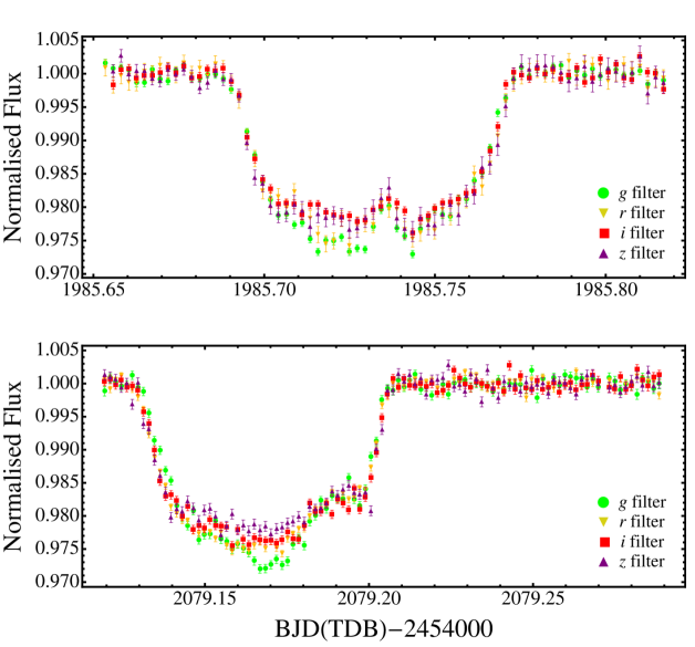
Figure 6: Combined four-colour transit light curves of HATS-2 obtained with the GROND imaging system. Green dots are for the data taken in the $g$ band, yellow upside down triangles for the $r$ band, red squares for the $i$ band, and purple triangles for the $z$ band. Top panel: transit observed on February 28, 2012. The bump observed just after the midtransit is interpreted as the covering of a “cold” starspot by the planet. Lower panel: transit observed on June 1, 2012. In addition to the bump occurred near the egress part of the light curve, a “hot” spot manifested in the $g$ band, just before the starting of the covering of the starspot.

4.1 Starspots and plages

From an inspection of Fig. 6, it is easy to note several distortions in the light curves. Such anomalies cannot be removed by choosing different comparison stars for the differential photometry, and we interpret them as the consequence of the planet crossing irregularities on the stellar photosphere, i.e. starspots. It is well known that starspots are at a lower temperature than the rest of the photosphere. The flux ratio should be therefore lower in the blue than the red. We thus expect to see stronger starspot features in the bluest bands.

The data taken on February 28, 2012, are plotted in the top panel of Fig. 6, where the bump, which is clearly present just after midtransit in all four optical bands, is explained by a starspot covered by the planet. In particular, considering the errorbars, the $g$, $r$, and $i$ points in the starspot feature look as expected, whereas the feature in $z$ is a bit peaked, especially the highest points at the peak of the bump at roughly BJD(TDB) 2455985.735. Before the starspot feature, it is also possible to note that the fluxes measured in the $g$ and $r$ bands are lower than those in the other two reddest bands, as if the planet were occulting a hotter zone of the stellar chromosphere. Actually, the most sensitive indicators of the chromospheric activity of a star in the visible spectrum are the emission lines of Ca II H$\lambda$3968, K$\lambda$3933, and H$\alpha$ $\lambda$6563, which in our case fall on the transmission wings of the $g$ and $r$ GROND passbands. The characterization of the chromospheric activity by calculating the Ca activity indicator using FEROS spectra was not possible due to high noise in the spectra.

Within the transit observed on June 1, 2012, whose data are plotted in the lower panel of Fig. 6, we detected another starspot, which occurred near the transit-egress zone of the light curve. Again, before the starspot feature, we note another “hotspot” in the $g$ band, which has its peak at roughly BJD(TDB) 2456079.681.

These hotspot distortions could be caused by differential color extinction or other time-correlated errors (i.e. red noise) of atmospheric origin. The g-band suffers most from the strength and variability of Earth-atmospheric extinction of all optical wavelengths covered by GROND, why the distortions in the g-band could have an atmospheric origin. Discrepancies in blue filters have been noted by other observers, and are often ascribed to systematic errors in ground-based photometry with these filters (e.g. Southworth et al., 2012). However, our group has observed more than 25 planetary transits with the GROND instrument to date, and in no other case have we seen similar features in the $g$-band only. We consider it unlikely that a systematic error of this form would only appear near to other spot features in the HATS-2 light curve, and therefore conclude that a more plausible scenario is that of a “plage”. A plage is a chromospheric region typically located near active starspots, and usually forming before the starspots appear, and disappearing after the starspots vanish from a particular area (e.g. Carroll & Ostlie, 1996). Accordingly, a plage occurs most often near a starspot region. As a matter of fact, in the GROND light curves, our plages are located just before each starspot. One can argue that the plage in the second transit is visible only in the $g$ band, but this can be explained by temperature fluctuations in the chromosphere, which causes a lack of ionized hydrogen, and by the fact that the Ca II lines are much stronger than the H$\alpha$ line for a K-type star like HATS-2. Another argument supporting this plage–starspot scenario is that, for these old stars, a solar-like relation between photospheric and chromospheric cycles is expected, the photospheric brightness varying in phase with that of the chromosphere (Lockwood et al., 2007).

We note, however, that if these are plages they must be rather different from solar plages, which are essentially invisible in broad-band optical filters unless they are very close to the solar limb. Detecting a plage feature through a broad-band filter near the stellar center suggests a much larger temperature contrast and/or column density of chromospheric gas than in the solar case.

4.2 Modelling transits and starspots

We modelled the GROND transit light curves of HATS-2 with the PRISM and GEMC codes (Tregloan-Reed et al., 2013). The first code models a planetary transit over a spotted star, while the latter one is an optimisation algorithm for finding the global best fit and associated uncertainties. Using these codes, one can determine, besides the ratio of the radii $R_{p}/R_{\star}$, the sum of the fractional radii, $r_{p}+r_{\star}=(R_{p}+R_{\star})/a$, the limb darkening coefficients, the transit midpoint $T_{0}$, and the orbital inclination $i_{p}$, as well as the photometric parameters of the spots, i.e. the projected longitude and the latitude of their centres ($\theta$ and $\phi$, these are equal to the physical latitude and longitude only if the rotation axis of the star is perpendicular to the line of sight), the spot size $r_{\mathrm{spot}}$ and the spot contrast $\rho_{\mathrm{spot}}$, which is basically the ratio of the surface brightness of the spot to that of the surrounding photosphere. Unfortunately, the current versions of PRISM and GEMC are set to fit only a single starspot (or hotspot), so we excluded the $g$-band dataset of the $2^{\mathrm{nd}}$ transit from the analysis, because it contains a hotspot with high contrast ratio between stellar photosphere and spot, which strongly interferes with the best-fitting model for the light curve.

Given that the codes do not allow the datasets to be fitted simultaneously, we proceeded as follows. First, we modelled the seven datasets ($1^{\mathrm{st}}$ transit: $g$, $r$, $i$, $z$; $2^{\mathrm{nd}}$ transit: $r$, $i$, $z$) of HATS-2 separately; this step allowed us to restrict the search space for each parameter. Then, we combined the four light curves of the first transit into a single dataset by taking the mean value at each point from the four bands at that point and we fitted the corresponding light curve; this second step was necessary to find a common value for $T_{0}$, $i_{p}$, $\theta$ and $\phi$. Finally, we fitted each light curve separately fixing the starspot position, the midtime of transit $T_{0}$ and the system inclination to the values found in the previous combined fit. While these parameters are the same for each band since they are physical parameters of the spot or the system and are therefore fixed during the analysis, other parameters as radius of the planet $R_{p}$, spot contrast $\rho_{spot}$ and temperature of the starspots $T_{spot}$ change according to the wavelength and hence according to the analysed band and are therefore free parameters during the fit.

The light curves and their best-fitting models are shown in Fig. 7, while the derived photometric parameters for each light curve are reported in Table 6, together with the results of the MCMC error analysis for each solution.

Table 6: Photometric parameters derived from the GEMC fitting of the GROND transit light curves.

$1^{\mathrm{st}}\,transit$
Parameter	Symbol	$g$	$r$	$i$	$z$
Radius ratio	$R_{p}/R_{\star}$	$0.1348\pm 0.0011$	$0.1324\pm 0.0011$	$0.13145\pm 0.00096$	$0.1352\pm 0.0010$
Sum of fractional radii	$r_{p}+r_{\star}$	$0.2204\pm 0.0018$	$0.2232\pm 0.0018$	$0.2149\pm 0.0016$	$0.2161\pm 0.0015$
Linear LD coefficient	$u_{1}$	$0.749\pm 0.060$	$0.593\pm 0.051$	$0.352\pm 0.057$	$0.298\pm 0.039$
Quadratic LD coefficient	$u_{2}$	$0.171\pm 0.018$	$0.296\pm 0.043$	$0.218\pm 0.028$	$0.144\pm 0.024$
Inclination (degrees) a	$i_{p}$	$85.26\pm 0.40$	$85.26\pm 0.40$	$85.26\pm 0.40$	$85.26\pm 0.40$
Longitude of spot (degrees) a,b	$\theta$	$5.78\pm 0.45$	$5.78\pm 0.45$	$5.78\pm 0.45$	$5.78\pm 0.45$
Latitude of Spot (degrees) a,c	$\phi$	$76.52\pm 1.94$	$76.52\pm 1.94$	$76.52\pm 1.94$	$76.52\pm 1.94$
Spot angular radius (degrees) d	$r_{\mathrm{spot}}$	$8.85\pm 0.61$	$10.01\pm 0.72$	$8.93\pm 0.65$	$8.72\pm 0.50$
Spot contrast e	$\rho_{\mathrm{spot}}$	$0.304\pm 0.035$	$0.546\pm 0.048$	$0.464\pm 0.052$	$0.251\pm 0.52$
$2^{\mathrm{nd}}\,transit$
Radius ratio	$R_{p}/R_{\star}$	$-$	$0.1356\pm 0.0012$	$0.13411\pm 0.00093$	$0.1307\pm 0.0011$
Sum of fractional radii	$r_{p}+r_{\star}$	$-$	$0.2108\pm 0.0019$	$0.2022\pm 0.0012$	$0.2039\pm 0.0017$
Linear LD coefficient	$u_{1}$	$-$	$0.473\pm 0.057$	$0.399\pm 0.049$	$0.252\pm 0.044$
Quadratic LD coefficient	$u_{2}$	$-$	$0.250\pm 0.038$	$0.230\pm 0.025$	$0.316\pm 0.049$
Inclination (degrees) a	$i_{p}$	$-$	$85.89\pm 0.40$	$85.89\pm 0.40$	$85.89\pm 0.40$
Longitude of spot (degrees) a,b	$\theta$	$-$	$35.26\pm 1.20$	$35.26\pm 1.20$	$35.26\pm 1.20$
Latitude of Spot (degrees) a,c	$\phi$	$-$	$80.60\pm 2.10$	$80.60\pm 2.10$	$80.60\pm 2.10$
Spot angular radius (degrees) d	$r_{\mathrm{spot}}$	$-$	$20.14\pm 1.49$	$17.79\pm 2.17$	$18.28\pm 2.31$
Spot contrast e	$\rho_{\mathrm{spot}}$	$-$	$0.753\pm 0.046$	$0.780\pm 0.054$	$0.789\pm 0.047$

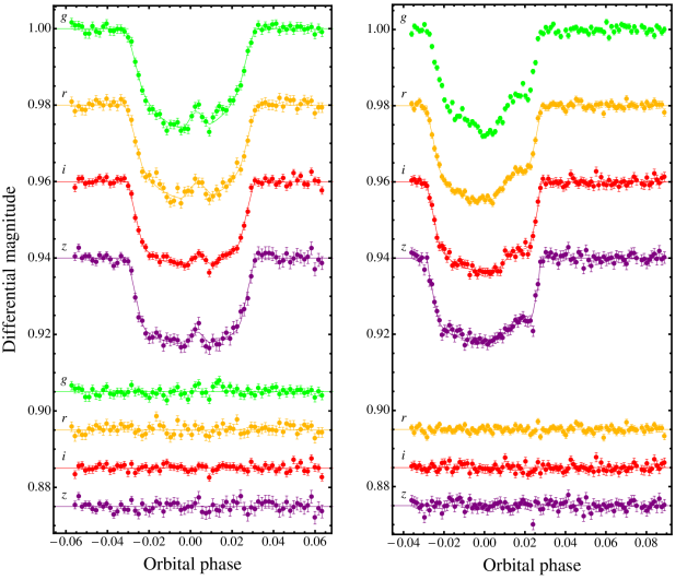
Figure 7: Phased GROND light curves of HATS-2b compared to the best GEMC fits. The light curves and the residuals are ordered according to the central wavelength of the filter used. Left panel: transit observed on February 28, 2012. Right panel: transit observed on June 1, 2012; due to to presence of the hotspot, the $g$ band was not analysed with GEMC (see text).

Comparing Table 5 with Table 6 we find that the fitted light curve parameters from the analysis described in Section 3.4 are consistent with the parameters that result from the GEMC+PRISM model, except for the inclination which differs by more than $2\sigma$. As already discussed in Section 3.4, the joint-fit analysis was performed both considering and without considering the points contaminated by the starspots, and the results are consistent with each other. So, our conclusion is that the spots themselves are not systematically affecting the stellar or planet parameters in a significant way; the differences in the inclination between GEMC and our joint fit are most likely due to differences in the modeling.

4.3 Starspots discussion

The final value for the starspots angular radii comes from the weighted mean of the results in each band and is $r_{\mathrm{spot}}=9.02^{\circ}\pm 0.30^{\circ}$ for the starspot in the $1^{\mathrm{st}}$ transit (spot #1) and $r_{\mathrm{spot}}=19.16^{\circ}\pm 1.08^{\circ}$ for the starspot in the $2^{\mathrm{nd}}$ transit (spot #2), with a reduced $\chi_{\nu}^{2}$ of 0.78 and 0.49 respectively, indicating a good agreement between the various light curves in each of the two transits. We note that the error of the angular size of the spot #2 is greater than that of the spot #1. While it may be that spot #2 is larger, we caution that its position near the limb of the star makes it size poorly constrained.

The above numbers translate to radii of $98\,325\pm 3\,876$ km and $208\,856\pm 11\,794$ km, which are equivalent $2.5\%$ and $11\%$ of the stellar disk, respectively. Starspot sizes are in general estimated by doppler-imaging reconstructions (i.e. Collier Cameron, 1992; Vogt et al., 1999) and their range is $0.1\%$ to $22\%$ of a stellar hemisphere, the inferior value being the detection limit of this technique (Strassmeier, 2009). Our measurements are thus perfectly reasonable for a common starspot or for a starspot assembly, and in agreement with what has been found in other K-type stars (e.g. TrES-1 (a K0V star) reveals a starspot of at least 42 000 km in radius, see Rabus et al. (2009)).

Starspots are also interesting in terms of how the contrast changes with passband. In particular, we expect that moving from ultraviolet (UV) to infrared (IR) wavelengths the spot becomes brighter relative to the photosphere. Considering the starspot #2, its contrast decreases from $r$ to $z$, even though this variation is inside the 1$\sigma$ error (see Table 6). Considering that HATS-2 has an effective temperature $T_{eff\star}=5227\pm 95$ K and modeling both the photosphere and the starspot as blackbodies (Rabus et al., 2009; Sanchis-Ojeda & Winn, 2011), we used Eq. (1) of Silva (2003) to estimate the temperature of the starspot #2 in each band:

$$f_{i}=\frac{\exp(h\nu/k_{B}T_{e})-1}{\exp(h\nu/k_{B}T_{0})-1}$$ (1)

with the spot contranst $f_{i}$, the Planck constant $h$, the frequency of the observation $\nu$, the effective surface temperature of the star $T_{e}$ and the spot temperature $T_{0}$. We obtained the following values: $T_{\mathrm{spot}\#2,r}=4916\pm 105$ K, $T_{\mathrm{spot}\#2,i}=4895\pm 121$ K and $T_{\mathrm{spot}\#2,z}=4856\pm 120$ K. The weighted mean is $T_{\mathrm{spot}\#2}=4891.5\pm 66.2$ K.

Unlike starspot #2, the spot contrasts for starspot #1 are inconsistent with expectations. The spot is too bright in $r$ relative to the other bandpasses, and too faint in $z$. If we estimate the starspot temperature in each band, we find $T_{\mathrm{spot}\#1,g}=4345\pm 97$ K, $T_{\mathrm{spot}\#1,r}=4604\pm 109$ K, $T_{\mathrm{spot}\#1,i}=4318\pm 128$ K and $T_{\mathrm{spot}\#1,z}=3595\pm 180$ K. While the temperature in $r$ is in agreement with those of $g$ and $i$ at $1-2\sigma$ level, and slight differences could be explained by chromospheric contamination (filaments, spicules, etc.), the temperature in $z$ seems physically inexplicable. This effect is essentially caused by the $z$ points at the peak of the starspot, at phase $\sim 0.004$ (see Fig. 7), which are higher than the other points. However, one has also to consider that errorbars in this band are larger than those found in the other bands. This is due to the fact that, since the GROND system design does not permit to chose different exposure times for each band, we are forced to optimize the observations for the $r$ and $i$ bands. Consequently, considering both the filter-transmission efficiency and the color and the magnitude of HATS-2, the SNR in these two bands is better than that in $z$, for which we have larger uncertainty in the photometry. Taking these considerations into account, we estimated the final temperature of starspot #1 neglecting the $z$-band value, and obtaining $T_{\mathrm{spot}\#1}=4425\pm 63$ K. In Fig. 8 the final values of the temperature contrast of the two starspots are compared with those of a sample of dwarf stars, which was reported by Berdyugina (2005). The derived contrast for the HATS-2 starspots is consistent with what is observed for other stars.

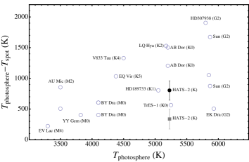
Figure 8: Spot temperature contrast with respect to the photospheric temperature in several dwarf stars. Gray square is from spot #2, black circle from spot #1, open circles from Berdyugina (2005), except TrES-1 (Rabus et al., 2009) and HD189733 (Sing et al., 2011). The name of the star and its spectral type is also reported for most of them. Nameless targets do not have a name in the publication of Berdyugina (2005) as well. Note that some stars appear two times.

As already observed by Strassmeier (2009), the temperature difference between photosphere and starspots can be not so different for stars of different spectral types. Moreover, in the case of long lifetime, the same starspot could been seen at quite different temperature (Kang & Wilson, 1989). It is then very difficult to find any clear correlation between starspot temperatures and spectral classes of stars.

The achieved longitudes of the starspots are in agreement with a visual inspection of the light curves. The latitude of starspot #1, $76.52^{\circ}\pm 1.94^{\circ}$, matches well with that of starspot #2, $80.6^{\circ}\pm 2.1^{\circ}$, the difference being within 1$\sigma$.

Multiple planetary transits across the same spot complex can be used to constrain the alignment between the orbital axis of the planet and the spin axis of the star (e.g. Sanchis-Ojeda et al., 2011). Unfortunately, from only two transits separated by 94 days we cannot tell whether or not the observed anomalies are due to the same complex. It is possible that they are. Following Solanki (2003) we estimate a typical lifetime of $\sim 130$ days for spots of the size seen here. Moreover the rotation period of $P_{\rm rot}=31\pm 1$ d inferred assuming they are the same spot is consistent with the value of $P_{\rm rot}=(30\pm 10\leavevmode\nobreak\ {\rm d})\sin i_{\star}$ estimated from the spectroscopically-determined sky-projected equatorial rotation speed. If they are the same spot complex, then the sky-projected spin-orbit alignment is $\lambda=8^{\rm\circ}\pm 8^{\rm\circ}$, which is consistent with zero. We caution, however, that this value depends entirely on this assumption which could easily be wrong. Continued photometric monitoring of HATS-2, or spectroscopic observations of the Rossiter-McLaughlin effect, are necessary to measure the spin-orbit alignment of this system.

To test whether the spot parameters inferred from modelling the transits are consistent with the amplitude of variations seen in the HATSouth photometry, we simulate a light curve using the Macula starspot model (Kipping, 2012) and the model parameters determined from the first GROND $r$-band transit. We find that such a spot gives rise to periodic variations with a peak-to-peak amplitude of $\sim 5$ mmag, which is within the 3.6 to 10.0 mmag range of amplitudes observed in the HATSouth light curve. The fact that the amplitude changes by a factor of $\sim 3$ over the course of the HATSouth observations indicates, however, that the spot(s) observed by HATSouth is(are) likely to be unrelated to the spot(s) observed with GROND.

5 Conclusions

In this paper we have presented HATS-2b, the second planet discovered by the HATSouth survey. This survey is a global network of six identical telescopes located at three different sites in the Southern hemisphere (Bakos et al., 2013). The parameters of the planetary system were estimated by an accurate joint fit of follow-up RV and photometric measurements. In particular, we found that HATS-2b has a mass of $1.369\pm 0.158$$M_{J}$, and a radius of $1.139\pm 0.025$$R_{J}$. To set this target in the context of other transit planet detections, we plotted 4 different types of correlation diagrams for the population of transiting planets (Fig. 9). We analysed the location of determined parameters for HATS-2b and its host star HATS-2 in the following parameter spaces: planetary radius $R_{p}$ vs. stellar radius $R_{\star}$, planetary mass $M_{P}$ vs. planetary equilibrium temperature $T_{eq,P}$, planetary radius $R_{p}$ vs. planetary equilibrium temperature $T_{eq,P}$, planetary radius $R_{p}$ vs. stellar effective temperature $T_{eff,\star}$, and planetary radius $R_{p}$ vs. planetary mass $M_{P}$. As illustrated in Fig. 9, the analysed parameter relations lie well within the global distribution of known exoplanets.

Within each correlation diagram, at least one well characterized exoplanet can be found, whose parameters are consistent with those of the HATS-2 system within the error bars. Looking on the correlation between planetary and stellar radius, the HATS-2 system is almost like the HAT-P-37 system (Bakos et al., 2012a). Comparing the planetary equlibrium temperature and planetary mass, HATS-2b is similar to TrES-2b (O’Donovan et al., 2006). The relation between planetary equilibrium temperature and planetary mass shows an agreement with WASP-32b (Maxted et al., 2010), while the relation between stellar effective temperature and planetary radius points out that HATS-2b agrees well with WASP-45b (Anderson et al., 2012) within the error bars. The focus on the planetary parameters radius and mass reveals a similarity to the transiting planet TrES-2. Comparing the atmospheres of exoplanets with similar physical parameters will be especially important to pursue with e.g. the future ECHO space mission (Tinetti et al., 2012).

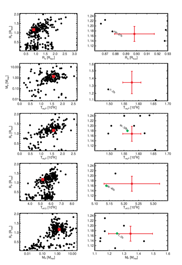
Figure 9: Correlation diagrams for confirmed transit planets (exoplanet.eu, last updated Jan 10 2013). From top to bottom: planetary radius $R_{p}$ vs. stellar radius $R_{\star}$, planetary mass $M_{P}$ vs. planetary equilibrium temperature $T_{eq,P}$, planetary radius $R_{p}$ vs. planetary equilibrium temperature $T_{eq,P}$, planetary radius $R_{p}$ vs. stellar effective temperature $T_{eff,\star}$ and planetary radius $R_{p}$ vs. planetary mass $M_{P}$. The position of the HATS-2 and HATS-2b parameters, respectively, are marked in red squares. Left panels give a global overview of the position of HATS-2 and HATS-2b in the population of known transit planets (black filled circles). Right panels illustrate a zoom in; green diamonds represent known exoplanets which fall within the errorbars of the HATS-2 system parameters. Short cuts: HP = HAT-P, W = WASP, T = TrES.

Very interesting is the detection of anomalies in the two multi-band photometric-follow-up light curves obtained with the GROND imaging instrument. We recognize the anomalies as starspots covered by HATS-2b during the two transit events, and used PRISM and GEMC codes (Tregloan-Reed et al., 2013) to re-fit the transit light curves, measuring the parameters of the spots. Both the starspots appear to have associated hot-spots, which appeared in the 1^st transit in the $g$ and $r$ bands, and only in the $g$ band in the 2^nd transit. These hotspots could be physically interpreted as chromospheric active regions known as plages, which can be seen only in the GROND’s bluest bands. We estimated the size and the temperature of the two starspots, finding values which are in agreement with those found in other G-K dwarf stars.