Non–equilibrium dynamics of a system with Quantum Frustration

Abstract

Using flow equations, equilibrium and non–equilibrium dynamics of a two–level system are investigated, which couples via non–commuting components to two independent oscillator baths. In equilibrium the two–level energy splitting is protected when the TLS is coupled symmetrically to both bath. A critical asymmetry angle separates the localized from the delocalized phase. On the other hand, real–time decoherence of a non–equilibrium initial state is for a generic initial state faster for a coupling to two baths than for a single bath.

I Introduction

Under the notations of frustration of decoherence or quantum frustration effects are subsumed which are ascribed to the competition and mutual cancellation of two environments, which couple to non–commuting observables of a central system. The notion was coined in Castro Neto et al. (2003) and the effect has since then been studied in a variety of systems, like a two–level system (TLS) coupled to two oscillator bath Castro Neto et al. (2003); Novais et al. (2005); Guo et al. (2012) or to two spin–baths Bhaktavatsala Rao et al. (2008), a harmonic oscillator coupled to two oscillator bath Kohler and Sols (2005, 2006); Cuccoli et al. (2010) in spin–lattices Cuccoli et al. or Josephson networks Giuliano and Sodano (2008). Most notably it was proposed as cooling mechanism Erez et al. (2008). The relation to Kondo physics was already pointed out in Castro Neto et al. (2003). Certain phenomena occuring in the two channel Kondo model or in the Bose–Fermi–Kondo model can actually be interpreted in terms of quantum frustration Zhu, Lijun and Si, Qimiao (2002); Zárand and Demler (2002).

In the model originally studied in Castro Neto et al. (2003); Novais et al. (2005), a TLS with energy gap $\Delta$ couples linearly with its two transversal components to two independent baths. It will be called 2BTLS in the following. The strength of the ohmic coupling is measured by two quantities $\gamma_{3}^{(1)}$ and $\gamma_{2}^{(2)}$ (assuming a magnetic field in $x$ direction, bath 1 couples to the $z$–component and bath 2 the $y$–component). One remarkable result of Ref. Castro Neto et al. (2003) were the renormalization group (RNG) equations

$$\frac{d\gamma_{3}^{(1)}}{dl} = -2\gamma_{3}^{(1)}\gamma_{2}^{(2)}-\gamma_{3}^{(1)}h^{2}\ ,$$

$$\frac{d\gamma_{2}^{(2)}}{dl} = -2\gamma_{3}^{(1)}\gamma_{2}^{(2)}-\gamma_{2}^{(2)}h^{2}$$

$$\frac{dh}{dl} = \left(1-\gamma_{3}^{(1)}-\gamma_{2}^{(2)}\right)h\ ,$$ (1)

where $dl=-d\ln\omega_{c}$ is the differential of the flow parameter and $h=\Delta/\omega_{c}$, where $\omega_{c}$ is the cutoff frequency of the bath modes. If either $\gamma_{3}^{(1)}$ or $\gamma_{2}^{(2)}$ is zero, the RNG equations of the single bath spin–Boson model A. J. Bray and N. A. Moore (1982); Chakravarty (1982) are recovered which predict a Kosterlitz Thouless phase transition for $\gamma=1$. For $\gamma_{3}^{(1)}$ $=$ $\gamma_{2}^{(2)}$ the renormalization flow is different: $h$ scales always to infinity, i. e. a phase transition never occurs, not even for arbitrary strong coupling. This is by now one of the most striking signature of quantum frustration.

However the question whether for large couplings the delocalized phase at symmetric coupling is stable against asymmetries remains unanswered by the above RNG equations. They do not yield any estimate for the renormalized energy gap $\Delta_{r}$, respectively Kondo temperature in the delocalized phase.

The body of publications, mentioned above focuses on thermal equilibrium. But the question whether or not quantum coherence of a non–equilibrium initial state is protected by quantum frustration is crucial for possible applications. Time evolution of a spin in non–equilibrium can be more complicated than exponential decay predicted by Bloch equations Slichter (1996). In particular an initially decoupled central system might on a very short time scale, called quantum Zeno–time, incur initial slips. This happens for instance to the dissipative harmonic oscillator F. Haake and R. Reibold (1985). In this case short times decoherence is indeed enhanced by a second bath and only later effects of quantum frustration occur Kohler and Sols (2005, 2006) .

We address the above questions for the 2BTLS using the method of Hamiltonian flow equations. Flow equations were introduced in the early nineties by Głazek and Wilson Głazek and Wilson (1993) and about the same time by Wegner Wegner (1994). The method rests upon a continuous diagonalization of the Hamiltonian, details can be found in Kehrein (2006). It was applied to the single bath spin–Boson model in Kehrein et al. (1996); Kehrein and Mielke (1996, 1997); Stauber and Mielke (2002). In particular it proved to yield good results for the renormalized energy gap $\Delta_{r}$.

In this work a generalization of equations (I) is derived analytically, which embraces any kind of coupling to two baths. Numerically $\Delta_{r}$ is calculated as a function of an asymmetry angle, called $\theta$, which varies from zero (single bath) to $\pi/4$ (completely symmetric). Whereas for weak coupling there is little dependence on the asymmetry angle, as the coupling becomes stronger the dependence on the asymmetry becomes more and more important. A symmetric coupling protects the gap and prevents the KT–phase transition. Identifying the critical angle allows us to plot a phase diagram in the $\gamma_{3}^{(1)}$–$\gamma_{2}^{(2)}$ plane, where the localized and the delocalized phases are separated by a critical line.

Using techniques developed recently Hackl and Kehrein (2008, 2009) we address the question whether decoherence of a non–equilibrium initial state is protected by a second bath. The answer to this can not be given without a careful distinction about what is meant by quantum decoherence. In a folkloristic definition decoherence is the decay of the off–diagonal elements in some pointer basis and relaxation the decay of the diagonal elements. For a two–level systems both processes are obviously not independent and it is therefore not easy to distinguish them.

For symmetric coupling we find that the moduli of off–diagonal elements in the eigenbasis of the spin operator in $x$–direction incur initial slips and subsequent oscillations on a time scale of the cutoff–frequency $\omega_{c}$. These initial slips on the time scale of $\omega_{c}$ are absent for a single baths, however the subsequent decay is oscillatory also in this case. The expectation value of the spin operator in $x$ direction behaves quite differently. Here the decay is initially faster for a single bath but slows down on the time scale of the Rabi frequency $\Delta^{-1}$. On the other hand for symmetric coupling the decay is initially slow but increases later to reach an equilibrium value, which is smaller than for a single bath.

In the first two sections of the manuscript we set up the model derive the flow equations and calculate equilibrium quantities. In section IV the non–equilibrium dynamics is considered.

II Flow equations for the 2BTLS

The Hamiltonian of the 2BTLS is given by

$$H^{(0)} = H_{0}+H_{I}^{(0)}$$

$$H_{0} = -\Delta S_{1}+\sum_{n=1}^{2}\sum_{k}\omega^{(n)}_{k}a_{n,k}^{\dagger}a_{n,k}$$ (2)

$$H_{\rm I}^{(0)} = S_{3}\otimes\sum_{k}\lambda^{(1)}_{3,k}\left(a_{1,k}+a_{1,k}^{\dagger}\right)+iS_{2}\otimes\sum_{k}\lambda^{(2)}_{2,k}\left(a_{2,k}-a_{2,k}^{\dagger}\right)$$

where $S_{i}$ are spin $\frac{1}{2}$–matrices and $a_{n,k}$ are bosonic annihilation operators $[a_{n,k},a_{m,k^{\prime}}^{\dagger}]$ $=$ $\delta_{kk^{\prime}}\delta_{nm}$ and $[a_{n,k},a_{m,k^{\prime}}]$ $=$ $[a_{n,k}^{\dagger},a_{m,k^{\prime}}^{\dagger}]$ $=$ $0$. We will also use $S_{0}=\frac{1}{2}{\mathbb{1}}_{2}$. The sum runs over the $N$ bath modes, where $N$ is assumed a large number such that the spectral functions

$$J_{3}^{(1)}(\omega) = \sum_{k}(\lambda_{3,k}^{(1)})^{2}\delta(\omega-\omega^{(1)}_{k})\ ,$$

$$J_{2}^{(2)}(\omega) = \sum_{l}(\lambda_{2,l}^{(2)})^{2}\delta(\omega-\omega^{(2)}_{l})$$ (3)

of both baths are smooth functions. They obey an Ohmic power law for small frequencies $J_{3}^{(1)}(\omega)$ $=$ $2\gamma_{3}^{(1)}\omega$ and $J_{2}^{(2)}(\omega)$ $=$ $2\gamma_{2}^{(2)}\omega$ and are regularized by a cutoff $\omega_{c}\gg\Delta$. For simplicity we assume here and in the following the cut–off and the number of bath modes to be the same for both baths.

The Hamiltonian is approximately diagonalized by a unitary transformation Wegner (1994); Kehrein (2006) which depends continuously on a flow parameter $B$. Any one–parameter family of unitarily equivalent Hamiltonians obeys the equation

$$\frac{d}{dB}H^{(0)}(B)=[\eta^{(0)}(B),H^{(0)}(B)]$$ (4)

with a properly chosen anti–Hermitian operator $\eta^{(0)}$. If $\eta^{(0)}$ is chosen as the commutator $\eta^{(0)}$ $=$ $[H_{0}(B),H_{I}^{(0)}(B)]$ it can be readily shown, see e. g. Wegner (2006) that if $H_{0}$ is non–degenerate in the limit $B\to\infty$, ${\rm tr}\,H(B)H_{I}^{(0)}\to 0$ and thus the Hamiltonian becomes diagonal. The commutator on the right hand side of equation (4) generates interaction terms not present in $H^{(0)}$. They are formally included in a more general Hamiltonian $H=H^{(0)}+H^{(1)}$ and in a new generator $\eta=[H_{0},H]$. The equations are closed by neglecting normal ordered products of more than two creation or annihilation operators.

In order to write the interacting part of the form invariant Hamiltonian $H$ in a compact form it is useful to arrange the creation and annihilation operators in a $4N$ vector $\vec{A\,}^{T}$ $=$ $(\vec{a_{1}}^{T},(\vec{a_{1}\,}^{\dagger})^{T},\vec{a_{2}\,}^{T},(\vec{a_{2}\,}^{\dagger})^{T})$, where $\vec{a\,}_{n}^{T}$ $=$ $(a_{n,1},\ldots,a_{n,N})$, $(\vec{a\,}^{\dagger}_{n})^{T}$ $=$ $(a^{\dagger}_{n,1},\ldots,a^{\dagger}_{n,N})$, $n=1,2$. It turns out useful as well to introduce coupling constants $\lambda_{\pm,k}^{(n)}$ $\equiv$ $\lambda_{3,k}^{(n)}\pm\lambda_{2,k}^{(n)}$ and arrange them in a $4N$ vector $\vec{\Lambda\,}$ = $(\vec{\lambda\,}_{+}^{(1)T},\vec{\lambda\,}_{-}^{(1)T},\vec{\lambda\,}_{+}^{(2)T},\vec{\lambda\,}_{-}^{(2)T})$, where $\vec{\lambda\,}_{\pm}^{(n)T}$$=$$(\lambda_{\pm,1}^{(n)},\ldots,\lambda_{\pm,N}^{(n)})$, $n=1,2$. Moreover $S_{\pm}=(S_{3}\pm iS_{2})/2$. Then

$$H_{\rm I} = S_{+}\otimes\vec{\Lambda\,}^{T}\vec{A}+S_{-}\otimes\vec{A\,}^{\dagger}\vec{\Lambda\,}+S_{1}\otimes:\vec{A\,}^{\dagger}T\vec{A\,}:$$ (5)

The symbol $:ab:$ denotes normal ordering with respect to a thermal expectation value. The $4N\times 4N$ matrix $T$ has the following block structure

$$T\ =\ \left(\begin{array}[]{cccc}s_{11}&t_{11}&s_{12}&t_{12}\cr t_{11}&s_{11}&t_{12}&s_{12}\cr s^{T}_{12}&t^{T}_{12}&s_{22}&t_{22}\cr t^{T}_{12}&s^{T}_{12}&t_{22}&s_{22}\end{array}\right)\ ,\quad t_{ii}=t_{ii}^{T},\quad s_{ii}=s_{ii}^{T},\quad t_{ij},s_{ij}\in{\mathbb{R}}\ .$$ (6)

Note the invariance of $T$ under the unitary automorphism $T\to\Sigma_{x}^{-1}T\Sigma_{x}$, where $\Sigma_{x}={\mathbb{1}}_{2}\otimes\sigma_{x}\otimes{\mathbb{1}}_{N}$ and $\sigma_{x}=\left[\begin{array}[]{cc}0&1\cr 1&0\end{array}\right]$ is a Pauli matrix. Likewise we define $\Sigma_{z}$. The generator reads

$$\eta = S_{+}\otimes\vec{\Lambda\,}^{T}\left(\Delta-\Omega\right)\vec{A\,}-S_{-}\otimes\vec{A\,}^{\dagger}\left(\Delta-\Omega\right)\vec{\Lambda\,}+S_{1}\otimes:\vec{A\,}^{\dagger}[\Omega,T]\vec{A\,}:\ ,$$ (7)

where $\Omega$ $=$ ${\rm diag}\,(\omega^{(1)},-\omega^{(1)},\omega^{(2)},-\omega^{(2)})$ and $\omega^{(n)}$ $=$ ${\rm diag}\,(\omega_{1}^{(n)},\ldots,\omega_{N}^{(n)})$, $n=1,2$. In former treatments of the Spin–Boson model with a single bath Kehrein et al. (1996); Kehrein and Mielke (1997) within the flow–equation approach, a formally simpler generator was used instead of the canonical one $\eta=[H_{0},H]$. This reduced the number of differential equations to be solved. The different generators were contrasted in Ref. Stauber and Mielke (2003).

In general there seem to exist by now no other guideline to improve the canonical generator than educated guess or physical intuition. Thus, for the present problem we stick to the canonical one.

The commutator $[\eta,H]$ is calculated straightforwardly and a set of non–linear coupled ODE’s is obtained for the tunnelling matrix element $\Delta$, the couplings $\vec{\Lambda}$ and for the matrix elements of $T$. They read

$$\frac{d\Delta(B)}{dB} = \frac{1}{2}\vec{\Lambda\,}^{T}\left(\Delta-\Omega\right)\coth\left(\frac{\beta|\Omega|}{2}\right)\vec{\Lambda\,}\ ,$$

$$\frac{d\vec{\Lambda}(B)}{dB} = -\left(\Delta-\Omega\right)^{2}\vec{\Lambda}+\left\{T(\Delta-\Omega)+[\Omega,T]\right\}\coth\left(\frac{\beta|\Omega|}{2}\right)\vec{\Lambda}\ ,$$

$$\frac{dT(B)}{dB} = -[\Omega,[\Omega,T]]-\frac{1}{2}\vec{\Lambda\,}\left(\Delta-\Omega\right)\vec{\Lambda\,}^{T}-\frac{1}{2}\Sigma_{x}\vec{\Lambda\,}\left(\Delta-\Omega\right)\vec{\Lambda\,}^{T}\Sigma_{x}\ .$$ (8)

The equations (8) form a set of $1+4N+2N(4N+1)$ first order non–linear differential equations which must be solved numerically. Before we do so, we show how they reduce to the RNG equations (II) for an ohmic bath in the low frequency limit. We limit ourselves to zero temperature. The differential equations for entries of $T$ are of the type

$$\frac{df(B)}{dB}\ =\ \omega f(B)+g(B)\ ,\qquad\omega\in{\mathbb{R}}$$ (9)

which can be solved exactly

$$f(B) = f(0)e^{\omega B}+\int_{0}^{B}dB^{\prime}e^{\omega(B-B^{\prime})}g(B^{\prime})\ .$$ (10)

This might be plugged into the flow equation for $\vec{\Lambda}$. It suffices to evaluate these equations for small frequencies. Using the definitions of the spectral functions (II) and

$$\sum_{k}\lambda_{j,k}^{(n)}(B)\lambda_{j^{\prime},k}^{(n)}(B^{\prime})\delta(\omega-\omega_{k}^{(n)})\ =\ 2\sqrt{\gamma_{j}^{(n)}\gamma_{j^{\prime}}^{(n)}}\omega\ ,\qquad\forall j,j^{\prime}\in\{2,3\}$$ (11)

an integro–differential equation for the coupling constants is acquired

$$\frac{d\gamma^{(n)}_{3}(B)}{dB} = -2\Delta(B)^{2}\gamma^{(n)}_{3}(B)-2\int_{0}^{B}dB^{\prime}\sqrt{\gamma^{(n)}_{3}(B)\gamma^{(n)}_{3}\left(B^{\prime}\right)}\omega_{c}^{2}$$ (12)

$$\qquad\qquad\times\int_{0}^{1}dxe^{-x\omega_{c}^{2}(B-B^{\prime})}\sum_{m=1}^{2}\left(\Delta(B)\sqrt{\gamma_{3}^{(m)}(B)}-2\omega_{c}\sqrt{\gamma_{2}^{(m)}(B)x}\right)$$

$$\qquad\qquad\qquad\times\left(2\Delta(B^{\prime})\sqrt{\gamma_{3}^{(m)}(B^{\prime})}-\omega_{c}\sqrt{\gamma_{2}^{(m)}(B^{\prime})x}\right)\ .$$

The corresponding equation for $\gamma^{(n)}_{2}$ is obtained from Eq. (12) by interchanging the indices $2$ and $3$ everywhere. This equation allows for a perturbative expansion in $h=\Delta/\omega_{c}$. Keeping only the highest order term in the integral Eq. (12) reduces to

$$\frac{d\gamma^{(n)}_{3}(B)}{dB} = -2\omega_{c}^{2}h^{2}(B)\gamma^{(n)}_{3}(B)-4\int_{0}^{B}dB^{\prime}\sqrt{\gamma^{(n)}_{3}(B)\gamma^{(n)}_{3}\left(B^{\prime}\right)}\omega_{c}^{4}$$ (13)

$$\qquad\qquad\times\int_{0}^{1}dxxe^{-x\omega_{c}^{2}(B-B^{\prime})}\sum_{m=1}^{2}\sqrt{\gamma_{2}^{(m)}(B)\gamma_{2}^{(m)}(B^{\prime})}\ .$$

In the limit $\omega_{c}\to\infty$ the $B^{\prime}$ integration becomes $\delta$–like for almost all $x\in[0,1]$ and we arrive at

$$\frac{d\gamma_{3}^{(n)}(B)}{dB} = -2\omega_{c}^{2}h^{2}(B)\gamma^{(n)}_{3}(B)-4\gamma_{3}^{(n)}(B)\omega_{c}^{2}\sum_{m=1}^{2}\gamma_{2}^{(m)}(B)$$ (14)

and likewise for $\gamma_{2}^{(n)}(B)$. To make contact with the RNG equations, we use the relation Kehrein (2006)

$$\omega_{c}\ =\ \frac{1}{2\sqrt{B}}\ =\ e^{-l}$$ (15)

and obtain

$$\frac{d\gamma_{2}^{(n)}(l)}{dl} = h^{2}\gamma_{2}^{(n)}-2\gamma_{2}^{(n)}\sum_{m=1}^{2}\gamma_{3}^{(m)}$$

$$\frac{d\gamma_{3}^{(n)}(l)}{dl} = h^{2}\gamma_{3}^{(n)}-2\gamma_{3}^{(n)}\sum_{m=1}^{2}\gamma_{2}^{(m)}\ ,\qquad n=1,2\ .$$ (16)

One derives straightforwardly from equation (8)

$$\frac{dh(l)}{dl}\ =\ \left(1-\sum_{j=2,3}\sum_{m=1}^{2}\gamma_{j}^{(m)}\right)h\ .$$ (17)

Equations (II) and (17) correspond to the one–loop perturbative renormalization group equations for arbitrary couplings $\gamma_{2}^{(n)}$ and $\gamma_{3}^{(n)}$, $n=1,2$. We do not analyze them further here, but only mention that the result of Novais et al. Novais et al. (2005) stated in Eq. (I) is obtained by setting $\gamma_{2}^{(1)}$ and $\gamma_{3}^{(2)}$ to zero. However it must be pointed out that the same equations are obtained for $\gamma_{3}^{(1)}$ and $\gamma_{2}^{(1)}$ , if $\gamma_{3}^{(2)}$ and $\gamma_{2}^{(2)}$ are set to zero, i. e.  in the absence of the second bath.

An adaptive step–size fourth order Runge–Kutta algorithm has proved to be a reliable solver of the flow equations (8). Most entries of $\vec{\Lambda}$ and of $T$ become exponentially small for large flow parameter and the Hamiltonian becomes diagonal

$$H(\infty)\ =\ -\Delta_{r}S_{1}+\frac{1}{2}:\vec{A\,}^{\dagger}|\Omega|\vec{A\,}:+H_{\rm res}$$ (18)

with a finite renormalized tunnelling matrix element $\Delta_{r}\equiv\Delta(\infty)$. Not all entries of $\vec{\Lambda}$ and of $T$ decay exponentially for large $B$. From the flow equations (8) it is seen that the coupling matrix elements $\lambda_{+,k}^{(n)}$ for frequencies close to the renormalized tunnelling matrix element decay most slowly. On the other hand the diagonal entries of $T$ do not decay at all, leading to an effective coupling of the bath modes to $S_{1}$ in the renormalized Hamiltonian

$$H_{\rm res}=S_{1}\otimes\sum\limits_{n=1}^{2}\sum_{k}s_{nn,kk}(\infty)a^{\dagger}_{n,k}a_{n,k}\ .$$ (19)

Although this term – being diagonal – causes no additional difficulties, for practical purposes it can be neglected, since the residual matrix elements $s_{11,kk}$, $s_{22,kk}$ are usually much smaller than the mean level spacing of the bath modes.

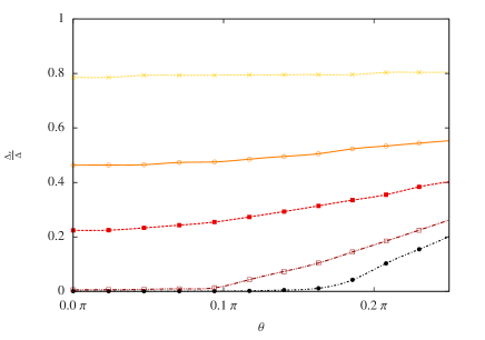
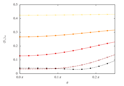
Figure 1: Left: Plot of the renormalized tunneling matrix element $\Delta_{r}$ as a function of the angle $\theta$ defined in the main text, the total coupling strength is $\gamma_{\rm tot}=0.1$ (crosses, online yellow), $\gamma_{\rm tot}=0.3$ (empty circles, online orange), $\gamma_{\rm tot}=0.5$ (filled boxes, online red), $\gamma_{\rm tot}=0.8$ (empty boxes, online dark red) and $\gamma_{\rm tot}=1$ (filled circles, full black line). The cutoff frequency is $\omega_{c}$ $=$ $10\Delta$. The number of bath modes is $N=1000$.
Right: the same for the equilibrium expectation value $\langle S_{1}\rangle$. $\omega_{c}$ $=$ $10\Delta$, $N=400$.

In figure 1 the renormalized energy gap of the two–level system is plotted for a fixed overall coupling $\gamma_{\rm tot}$ $\equiv$ $\gamma_{3}^{(1)}+\gamma_{2}^{(2)}$ as a function of the relative angle $\theta\equiv\arctan\left(\sqrt{\gamma_{2}^{(2)}/\gamma_{3}^{(1)}}\right)$ which varies from zero (single bath) to $\pi/4$ (equal coupling strength). Whereas for small overall coupling the renormalized energy gap $\Delta_{r}$ is almost independent of $\theta$, for increasing coupling strength the gap is protected by a symmetric coupling. Finally for $\gamma_{\rm tot}$ $=1$ the energy gap renormalizes to zero for $\theta=0$ but remains finite for symmetric coupling.

If $\gamma_{\rm tot}$ is increased even further the energy gap $\Delta(B)$ crosses zero for some large value of $B$ and decays afterwards very slowly in an oscillatory fashion to zero. This happens for angles smaller than some critical angle, indicating the onset of the strong coupling regime, respectively of the KT phase transition. It is expected that the flow equations, being generically perturbative, become less exact for stronger coupling. However for $\theta=0$ the critical value $\gamma=1$ was obtained analytically and with good precision numerically Kehrein et al. (1996) . Therefore it is well justified to assume that the flow equations yield a good estimates for the critical $\gamma_{\rm tot}$ for $\theta\neq 0$ as well.

In figure 2 the critical line is plotted in the $\gamma_{\rm tot}$ – $\theta$ plane, which separates the localized from the delocalized phase. It is seen that it crosses the $x$–axis at some value smaller than one. This offset is due to the finite number of bath modes and of the finite cutoff frequency. This can be improved systematically by increasing the number of bath modes and simultaneously increasing the endpoint of the flow $B_{\rm max}$. For values of $\gamma_{\rm tot}$ larger a than some value $\gamma_{\rm tot}\approx 2.5$ the flow becomes unstable.

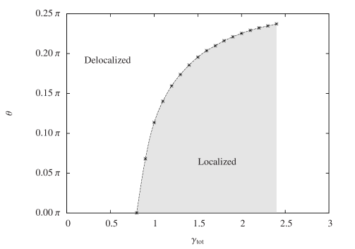
Figure 2: Phase diagramm in the $\gamma_{\rm tot}$ – $\theta$ plane. The line indicates the critical asymmetry angle, which separates the localized from the delocalized phase. The critical angle was determined for $N=800$ bath modes.

III Equilibrium expectation values

In oder to calculate equilibrium expectation values with respect to the transformed Hamiltonian $H(\infty)$ the corresponding operators have to transform as well. Complex $4N$–vectors $\vec{\chi\,}$ and $\vec{\zeta\,}_{0,1}$ are introduced and the spin operators are expanded as

$$S_{1} = h_{0}S_{0}+h_{1}S_{1}+S_{+}\otimes\vec{\chi\,}^{\dagger}\vec{A}+S_{-}\otimes\vec{A\,}^{\dagger}\vec{\chi\,}$$

$$S_{+} = h_{+}S_{+}+h_{-}S_{-}+S_{0}\otimes\vec{\zeta\,}_{0}^{\dagger}\vec{A}+S_{1}\otimes\vec{\zeta\,}_{1}^{\dagger}\vec{A}$$

$$S_{-} = h_{-}^{*}S_{+}+h_{+}^{*}S_{-}+S_{0}\otimes\vec{A\,}^{\dagger}\vec{\zeta\,}_{0}+S_{1}\otimes\vec{A\,}^{\dagger}\vec{\zeta\,}_{1}$$ (20)

The flow equations for $h_{0}$, $h_{1}$, $h_{\pm}$ and for $\vec{\chi\,}$, $\vec{\zeta\,}_{0,1}$ are obtained by calculating the commutator $[\eta,S_{i}]$. The equations are closed by neglecting all normal ordered operator products with two or more annihilation or creation operators. They are stated in App. B. The equilibrium density matrix with respect to the renormalized free Hamiltonian (18) is just

$$\rho_{\rm eq}\ =\ \left(S_{0}+\tanh\left(\frac{\Delta_{r}\beta}{2}\right)S_{1}\right)\otimes\rho^{(1)}_{\rm eq}\otimes\rho^{(2)}_{\rm eq}\ .$$ (21)

Here $\rho^{(n)}_{\rm eq}$ $=$ $\prod_{k}\exp(-\beta\omega_{k}^{(n)}a_{n,k}^{\dagger}a_{n,k})/$ is the thermal density matrix of the two free environments. Thus, once the equations are numerically solved, an arbitrary equilibrium expectation value of the spin operators is readily calculated. As an example we consider the one–sided Fourier transform

$$\chi_{zz}(\omega)\ =\ -i\int_{0}^{\infty}\frac{dt}{2\pi}e^{i\omega t}\left<[S_{3}(0),S_{3}(t)]\right>$$ (22)

of the correlator $\left<[S_{3}(0),S_{3}(t)]\right>$ which was investigated in Novais et al. (2005). At zero temperature, its imaginary part $\chi_{zz}^{\prime\prime}$ is given by

$$\chi^{\prime\prime}_{zz}(\omega) \propto \left(h_{+}+h_{-}\right)^{2}\delta\left(\omega-\Delta_{r}\right)+\left(\vec{\zeta\,}_{0}+\vec{\zeta\,}_{1}\right)^{\dagger}\left(1+\Sigma_{x}\right)\delta\left(\omega-|\Omega|\right)\left(\vec{\zeta\,}_{0}+\vec{\zeta\,}_{1}\right)\ .$$ (23)

As a second example, we consider the equilibrium expectation value

$$\langle S_{1}\rangle\ =\ \frac{h_{0}}{2}+\frac{h_{1}}{2}\tanh\left(\frac{\Delta_{r}\beta}{2}\right)\ .$$ (24)

It is plotted in the bottom picture of figure 1 for zero temperature and for different angles $\theta$ as defined before. Since the calculation is numerically more expensive than that of the energy gap, the number of bath modes is $N=400$. For small and intermediate coupling it behaves qualitatively similar to the renormalized two–level energy gap $\Delta_{r}$. For strong coupling $\gamma_{\rm tot}$ $\approx$ $1$ it is seen that $\langle S_{1}\rangle$ does not scale to zero for $\theta=0$ as expected, indicating that the flow equations lose accuracy in the strong coupling regime.

Before we discuss the numerical results for the equilibrium correlation functions an explanatory remark is in order. A careful treatment of equilibrium correlation functions within the flow–equation approach requires high sophistication. For frequencies close to the renormalized tunnel matrix element $\Delta_{r}$ the flow converges only very slowly with $B_{\rm max}$, the endpoint of the numerical integration of the flow. Since the endpoint of the integration is itself limited by the density of the bath modes an accurate resolution would require an out of scale number of bath modes. As a consequence of this numerical limitation the equilibrium correlation functions have a two–peak structure: one broad maximum at a value smaller than $\Delta_{r}$ and a second sharp peak right at $\Delta_{r}$, which is clearly unphysical.

The problem can be overcome by employing constants of motion under the flow. This was done in Kehrein and Mielke (1997) for the one–bath spin Boson model. The result is a smooth curve with a single peak. But such constants of motion under the flow are not always easy to identify.

We refrain from this procedure and show the curves for $\chi^{\prime\prime}_{zz}(\omega)$ obtained by fitting the numerical data with smoothing splines using an extremely high fidelity factor (of order $10^{8}$) everywhere but around $\Delta_{r}$, where it is quartically suppressed.

In figure 3 the correlation function $\chi^{\prime\prime}_{zz}(\omega)$ is plotted for equal coupling strength to both baths and with an overall coupling strength $\gamma_{\rm tot}$ varying between $0.1$ and one. The curve corresponds to Fig. 4 in reference Novais et al. (2005) and is qualitatively similar. As the coupling strength increases the resonance peak becomes smaller and smaller but never disappears. The maximum of the resonance peak is systematically below $\Delta_{r}$. This is a difference to Fig. 4 in reference Novais et al. (2005) where the maximum seems to be always right at the renormalized tunnel matrix element.

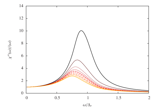
Figure 3: Plot of the transverse susceptibility $\chi_{zz}^{\prime\prime}(\omega)/\omega$ in $z$–direction for symmetric coupling $\gamma_{3}^{(1)}$ $=$ $\gamma_{2}^{(2)}$ and for ten different values of $\gamma_{\rm tot}$ $=\sqrt{2}\cdot 0.1\,n$, $1\leq n\leq 10$, from top to bottom (online color: from dark–colored to light–colored). The number of bath modes is 400, $\Delta/\omega_{c}$ $=$ $1/10$.

In figure 3 the correlation function $\chi^{\prime\prime}_{zz}(\omega)$ is plotted for fixed overall coupling strength $\gamma_{\rm tot}$ and for different angles $\theta$. The resonance peak in the symmetric case ($\theta=\pi/4$) is largely enhanced as compared to the highly asymmetric case ($\theta=0.1\pi$). However, the reason for this is rather trivial. In the highly asymmetric case the coupling to the $z$–component is largest, whereas there is no coupling to the $y$–component. In the symmetric case the coupling to the $z$–component is reduced, which is reflected by the enhanced resonance peak of $\chi^{\prime\prime}_{zz}$. However the coupling to the $y$–component is larger, which yields a reduced resonance peak of $\chi^{\prime\prime}_{yy}$ (not shown here). If we write $\chi^{\prime\prime}_{zz}(\omega,\theta)$ as a function of the relative angle $\theta$, then the obvious relation $\chi^{\prime\prime}_{zz}(\omega,\theta)$ $=$ $\chi^{\prime\prime}_{yy}(\omega,\pi/2-\theta)$ holds. Thus an enhancement of the resonance peak in $z$–direction comes necessarily with a decrease in $y$–direction and vice versa. Indeed in Fig. 3 the resonance peak of $\chi^{\prime\prime}_{zz}$ is biggest for $\theta=0.3\pi$ in spite of the asymmetric coupling (for even higher $\theta$ it increases more and more). Note however that the location of the maximum of the peak is maximal in the symmetric case.

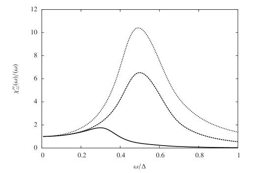
Figure 4: Plot of the transverse susceptibility $\chi_{zz}^{\prime\prime}(\omega)/\omega$ in $z$–direction for three different angles $\theta$ $=0.1\pi$ (full line), $\theta$ $=\pi/4$ (dashed line) and $\theta$ $=0.3\pi$ (dotted line) for overall coupling strength $\gamma_{\rm tot}=0.3$. The number of bath modes is $N=400$, $\omega_{c}/\Delta=$$10$.

IV Thermalization and Decoherence

In thermal equilibrium the mutual energy transfer from the system to the environment and vice versa is zero, warranted by fluctuation dissipation theorems. However in the process of thermalization the net energy transfer of the system to the environment is positive.

Assuming an decoupled initial state, which is fully polarized in some direction perpendicular to the $x$ axis (we may assuume $0\leq\theta^{\prime}\leq\pi/4$)

$$\rho_{\rm init}\ =\ \left(S_{0}+\cos\theta^{\prime}S_{3}+\sin\theta^{\prime}S_{2}\right)\otimes\rho^{(1)}_{\rm eq}\otimes\rho^{(2)}_{\rm eq}\ ,$$ (25)

thermalization is characterized by the time evolution of the expectation value of the system’s energy $\langle H_{S}(t)\rangle$ $=$ $-\Delta\langle S_{1}(t)\rangle$ . This quantity is expected to approach its equilibrium value on a certain time scale, the so called relaxation time, which is usually denoted $T_{1}$.

Decoherence is the creation of entanglement of the system with the environment. It is measured by the decay of the off–diagonal elements of the reduced density matrix of the spin in the $S_{1}$ basis, i. e. by the expectation values $\langle S_{\pm}\rangle$. A basis independent measure for decoherence is the purity ${\cal P}(t)$ $=$ ${\cal P}_{\parallel}(t)$ $+{\cal P}_{\perp}(t)$, where ${\cal P}_{\parallel}(t)$ $=$ $2\sum_{n=0}^{1}\langle S_{n}(t)\rangle^{2}$ and ${\cal P}_{\perp}(t)$ $=$ $2\sum_{n=2}^{3}\langle S_{n}(t)\rangle^{2}$. Decay of decoherence takes place on a time scale $T_{2}$, called decoherence time Slichter (1996), we asociate it with ${\cal P}_{\perp}(t)$. Both decoherence time and relaxation time enter in the definition of purity. We call the two quantities ${\cal P}_{\perp}(t)$ and ${\cal P}_{\parallel}(t)$ transverse respectively parallel purity. For the initial state (25) ${\cal P}_{\perp}(0)$ $={\cal P}_{\parallel}(0)$ $=1/2$.

Assuming a decoupled initial state as in Eq. (25) first order differential equations for the spin expectation values are straightforwardly derived in second order perturbation theory

$$\frac{d}{dt}\langle S_{1}\rangle = -\left(\Gamma^{(2)}_{2}(t)+\Gamma^{(1)}_{3}(t)\right)\langle S_{1}\rangle-F(t)$$

$$\frac{d}{dt}\langle S_{2}\rangle = \tilde{\Delta}^{(1)}_{3}(t)\langle S_{3}\rangle-\Gamma^{(1)}_{3}(t)\langle S_{2}\rangle$$

$$\frac{d}{dt}\langle S_{3}\rangle = -\tilde{\Delta}^{(2)}_{2}(t)\langle S_{2}\rangle-\Gamma^{(2)}_{2}(t)\langle S_{3}\rangle\ ,$$ (26)

with the time–dependent coefficients

$$\Gamma^{(m)}_{n}(t) = \int\limits_{0}^{t}dt^{\prime}\int\limits_{0}^{\infty}d\omega\cos\left(\Delta(t^{\prime}-t)\right)\cos\left(\omega(t-t^{\prime})\right)J^{(m)}_{n}(\omega)\coth\left(\omega\beta/2\right)$$

$$\tilde{\Delta}^{(m)}_{n}(t) = \Delta-\int\limits_{0}^{t}dt^{\prime}\int\limits_{0}^{\infty}d\omega\sin\left(\Delta(t^{\prime}-t)\right)\cos\left(\omega(t-t^{\prime})\right)J^{(m)}_{n}(\omega)\coth\left(\omega\beta/2\right)$$

$$F(t) = \int\limits_{0}^{t}dt^{\prime}\int\limits_{0}^{\infty}d\omega\sin\left(\omega(t-t^{\prime})\right)\sin\left(\Delta(t^{\prime}-t)\right)\left(J^{(2)}_{2}(\omega)+J^{(1)}_{3}(\omega)\right)\ .$$ (27)

In the Markov approximation these coefficients become time independent $\Gamma^{(m)}_{n}(t)=\Gamma^{(m)}_{n}$ $=(\pi/2)J^{(m)}_{n}(\Delta)\coth(\beta\Delta/2)$, $F(t)=F=(\pi/2)(J^{(2)}_{2}(\Delta)+J^{(1)}_{3}(\Delta))$ and $\tilde{\Delta}^{(m)}_{n}(t)=$ $\tilde{\Delta}^{(m)}_{n}=$ $\Delta-\Delta\int_{0}^{\omega_{c}}d\omega$ $\coth(\beta\omega/2)$ $J^{(m)}_{n}(\omega)/(\omega^{2}-\Delta^{2})$. Note that for an ohmic bath and at zero temperature $\tilde{\Delta}^{(m)}_{n}$ has a logarithmic singularity in the cutoff frequency $\omega_{c}$.

From equations (IV) the phenomenological Bloch equations are obtained which predict an exponential decay of decoherence and of relaxation. Their solutions are

$$\langle S_{1}(t)\rangle = (\langle S_{1}(0)\rangle-\langle S_{1}\rangle_{\rm eq})e^{-(\Gamma^{(2)}_{2}+\Gamma^{(1)}_{3})t}+\langle S_{1}\rangle_{\rm eq}$$

$$\langle S_{n}(t)\rangle = \frac{\lambda_{+}\langle S_{n}(0)\rangle+i\langle\dot{S}_{n}(0)\rangle}{\lambda_{+}-\lambda_{-}}e^{i\lambda_{-}t}-\frac{\lambda_{-}\langle S_{n}(0)\rangle+i\langle\dot{S}_{n}(0)\rangle}{\lambda_{+}-\lambda_{-}}e^{i\lambda_{+}t}$$ (28)

where $\lambda_{\pm}$ are the roots of the characteristic polynomial

$$\chi(\omega)\ =\ \omega^{2}-i\omega(\Gamma^{(2)}_{2}+\Gamma^{(1)}_{3})+\tilde{\Delta}^{(2)}_{2}\tilde{\Delta}^{(1)}_{3}-\Gamma^{(2)}_{2}\Gamma^{(1)}_{3}$$ (29)

Thus decoherence and relaxation time are given by $T_{1}=1/(\Gamma^{(2)}_{2}+\Gamma^{(1)}_{3})$ and $T_{2}$$=$ $2T_{1}$. In second order perturbation theory the friction coefficients of the two baths add up. No frustration occurs.

In the Markov approximation Bloch equations hold beyond perturbation theory with relaxation and decoherence times depending in a more complicated non–perturbative way on the coupling strength $\gamma^{(1)}_{3}$ and $\gamma^{(2)}_{2}$. Corrections were calculated in Ref. Novais et al. (2005). In the regime where the Bloch equations (IV) hold, the quantum regression theorem can be invoked and the dynamics of the expectation values is governed by the equilibrium correlation functions.

Yet at low temperature and on the time scale of the inverse cutoff frequency, Bloch equations do not hold. The coefficients in Eq. (IV) become time dependent and the simple exponential behavior (IV) breaks down. This is seen most directly in a Taylor expansion of the time–evolution operator $U(t)=1-iHt-t^{2}H^{2}/2+{\cal O}(t^{3})$. For the initial state (25) it predicts a quadratic behavior of $\langle S_{1}\rangle=$ $t^{2}/2\tau^{2}+{\cal O}(t^{3})$, where $\tau^{-1}$ $\approx$ $\omega_{c}\sqrt{\gamma^{(1)}_{3}+\gamma^{(2)}_{2}}$ is the inverse quantum Zeno time. For the transverse purity one obtains

$$2P_{\perp}(t)\ =\ 1-\frac{t^{2}}{\tau^{2}}\left\{\sin^{2}(\theta)\cos^{2}(\theta^{\prime})+\sin^{2}(\theta)\cos^{2}(\theta^{\prime})\right\}+{\cal O}(t^{3})$$ (30)

The quadratic time dependence vanishes iff $\theta=\theta^{\prime}$ $=0$. This indicates that initially, for short times, a symmetric coupling accelerates decay of coherence.

In order to monitor the time evolution of the expectation values in the transient regime on a time scale of order of the quantum Zeno time, methods of non–equilibrium real time thermodynamics must be employed. Real time quantum evolution is addressed within the flow equation approach Hackl and Kehrein (2008, 2009) by applying subsequently the unitary transformation $U_{B}(B_{1},B_{2})$ generated by $\eta(B)$ and the time evolution operator $U_{t,\infty}(t_{1},t_{2})=e^{-iH(\infty)(t_{1}-t_{2})}$ on the operator of interest according to the diagramm:

Since time evolution is simple for $B=\infty$ the observables are first transformed into the $B=\infty$ basis evolve in time and are then transformed back. At time $t$ the Heisenberg operators have been propagated by the diagonalized Hamiltonian (18). This yields new time dependent expansion coefficients $\tilde{h\,}_{\pm}(t)$$=$ $e^{\pm i\Delta_{r}t}h_{\pm}(\infty)$, $\vec{\tilde{\chi}\,}(t)$ $=$ $e^{i(\Delta_{r}-\Omega)t}$ $\vec{\chi}(\infty)$ and $\vec{\tilde{\zeta}\,}_{n}(t)$ $=$ $e^{i\Omega t}\vec{\zeta}_{n}(\infty)$, $n=0,1$. The coefficients $h_{0}=\tilde{h\,}_{0}$ and $h_{1}=\tilde{h\,}_{1}$ remain constant under time evolution. These coefficients are numerically transformed back, yielding an approximate solution of the Heisenberg equation for the spin operators. The expectation value with respect to the density matrix (25) are

$$\langle S_{1}(t)\rangle = \tilde{h}_{0}(t)/2$$

$$\langle S_{2}(t)\rangle = {\rm Im}\left[(\tilde{h}_{+}(t)-\tilde{h}^{*}_{-}(t))e^{i\theta^{\prime}}/2\right]$$

$$\langle S_{3}(t)\rangle = {\rm Re}\left[(\tilde{h}_{+}(t)+\tilde{h}^{*}_{-}(t))e^{i\theta^{\prime}}/2\right].$$ (31)

The calculation is numerically delicate Hackl and Kehrein (2008, 2009). In order to perform the backward integration the forward flow of the Hamiltonian must be stored. This is a sizable amount of data of order of one terabyte. The read–in and the read–out slow down the routine. We thus performed the calculation of ${\cal P}_{\perp}$ with 250 bath modes, respectively of $\langle S_{x}(t)\rangle$ with 100 bath modes.

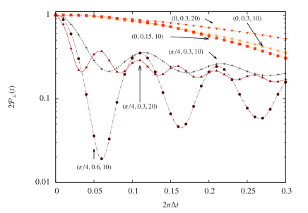
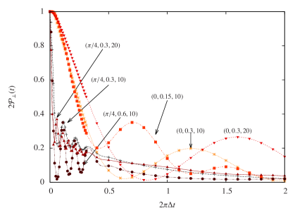
Figure 5: Right: Time evolution of the transversal purity for an initial state characterized by the angle $\theta^{\prime}=0$ for different triplets $(\theta,\gamma_{\rm tot},\omega_{c}/\Delta)$. These are $(\pi/4,0.3,10)$ (online black, crosses), $(0,0.3,10)$ (online yellow, asterisks), $(0,0.15,10)$ (online light red, boxes), $(\pi/4,0.6,10)$ (online dark purple, dots), $(\pi/4,0.3,20)$ (online lighter purple, triangles), $(0,0.3,20)$ (online darker red, triangles).
Left: The same for short times on a logscale.

In figure 5 the transverse purity is plotted for different values of $\gamma_{3}^{(1)}$ and $\gamma_{2}^{(2)}$ for an initial state characterized by the angle $\theta^{\prime}=0$. It is seen that for short times of order of $\omega_{c}^{-1}$ the transverse purity decays faster for a symmetric coupling than for a single bath, as predicted by equation (30). The decay occurs in an oscillatory fashion for both a single bath and for symmetric ccoupling. Although the dissipative two–level system has been studied extensively Leggett et al. (1987) to our best knowledge this oscillatory purity revival was not reported before. By now we do not have a satisfactory physical explanation for it. For symmetric coupling the oscillations decrease rapidly in less than one period of the Rabi oscillations. As can be seen from left picture of Fig. 5 the frequency seems to scale with $\omega_{c}$ and the amplitudes with $\gamma_{\rm tot}$. For a single bath the oscillations are much slower and decay less rapidly.

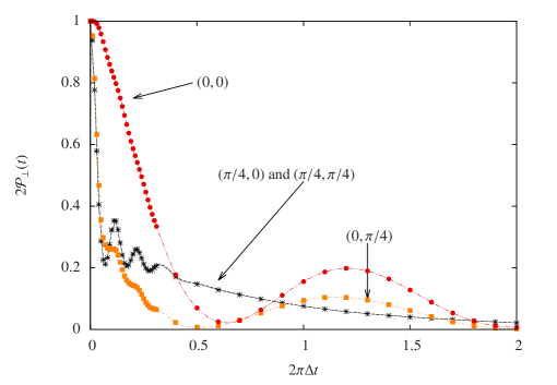
Figure 6: Time evolution of the transversal purity for an initial state characterized by the angles $\theta^{\prime}=0,\pi/4$ for symmetric coupling (asterisks, online black) and for a single bath, $\theta^{\prime}$ $=0$ (dotted, online red) and $\theta^{\prime}$ $=\pi/4$ (boxed, online orange). The other parameters are $\gamma_{\rm tot}=0.3$ and $\omega_{c}/\Delta$ $=10$.

The dependence on the initial state is considered in Fig. 6. The transverse purity for the initial state characterized by $\theta^{\prime}=0$ and for the initial state $\theta^{\prime}=\pi/4$ is plotted. Whereas for symmetric coupling there is no visible difference, for a single bath the initial decay is much faster for $\theta^{\prime}=\pi/4$ than for $\theta^{\prime}=0$, see Eq. (30).

The time evolution of $\langle S_{x}(t)\rangle$ is plotted in Fig. 7 for symmetric coupling ($\theta=\pi/4$) and for a single bath ($\theta=\pi/4$) for a moderate overall coupling strength $\gamma_{\rm tot}=0.3$. Here the expectation value indeed decays initially faster for a single bath than for symmetric coupling. However on a time scale of the Rabi–oscillations the decay grows faster for symmetric coupling to reach an equilibrium value, which is smaller than for a single bath in accordance with Fig. 1.

Figure 7: Time evolution of the expectation value $\langle S_{x}(t)\rangle$ for the initial state (25) for symmetric coupling (online blue, stars) and for a single bath (online red, crosses), $\gamma_{\rm tot}=0.3$, $\omega_{c}/\Delta$$=10$.

V Summary & Discussion

While the calculation of equilibrium correlation functions is somewhat cumbersome within the flow equation approach, the method turns out to be a useful numerical tool in non–equilibrium physics. We were able to monitor purity decay on the time scale of the quantum Zeno time as well as on the time scale of the inverse Rabi frequency.

When one speaks about coherence of a two–level system one has carefully to distinguish between the decay of the off–diagonal elements and of the diagonal elements. It is characteristic for a small size Hilbert–space that both are not independent and the distinction between decoherence and dissipation is fuzzy.

In our analysis frustration effects of two independent oscillator bath could be identified in the renormalized energy gap $\Delta_{r}$, in the ground state expectation value of $S_{1}$ and in the ground state energy shift. These quantities are protected by a symmetric coupling. In particular the protection of $\langle S_{1}\rangle$ can rightly be called protection of decoherence since it contributes to a high equilibrium purity of the spin.

In non–equilibrium relaxation, i. e. the decay of $\langle H_{S}\rangle$ $\propto$ $-\langle S_{1}\rangle$, is protected by a symmetric coupling on a time scale of the quantum Zeno time. However, the decay of the off–diagonal matrix elements of the reduced density matrix, corresponding to $\langle S_{2}\rangle$, $\langle S_{3}\rangle$ and to the transverse purity is systematically faster for a symmetric coupling.

The decay of both $\langle H_{S}\rangle$ and of the transverse purity occurs in an oscillatory fashion. The physical reason behind these oscillations is unclear.

The dependence of the renormalized energy gap $\Delta_{r}$ on an asymmetry angle is a generic non perturbative effect. The flow equations (8) might be truncated by setting all second order terms,  i. e. the matrix entries of $T$ (Eq. (6)), to zero. The truncated flow equations can be analyzed analytically, see App. A. The outcome is $\ln(\Delta_{r}/\Delta)$ $\propto-\gamma_{\rm tot}/(1-\gamma_{\rm tot})$, similar to the old result by Silbey and Harris Silbey and Harris (1983) which features no dependence on the asymmetry angle. Our analysis affirms that the delocalized phase for couplings $1<\gamma_{\rm tot}<\infty$ is stable against small asymmetries.

The perturbative RNG equations (II) and (17) obtained from the flow equations are completely symmetric in the four coupling constants $\gamma_{2}^{(n)}$, $\gamma_{3}^{(n)}$, $n=1,2$. Setting any two of them to zero yields the RNG equations of Ref. Castro Neto et al. (2003), with the implication of a delocalized phase for $\gamma_{\rm tot}$ $\to\infty$. Setting for instance $\gamma_{2}^{(2)}=$$\gamma_{3}^{(2)}$ $=0$, this implys that also a symmetric coupling of the spin with its $y$ and $z$ components to a single bath can protect the delocalized phase. This question requires further investigation.

Appendix A Linearized Flow equations for two baths

We consider the linearized version of the flow equations. In the linearized version of the flow equations the flow of $T$ can be neglected.

$$\frac{d\vec{\Lambda\,}(B)}{dB} = -\left(\Delta-\Omega\right)\vec{\Lambda}$$ (32)

For ohmic spectral functions $J_{i}^{(n)}(\omega)$ $=$ $2\gamma_{i}^{(n)}\omega\theta(\omega_{c}-\omega)$ , $i=2,3$, $n=1,2$ immediately the first order RG equations

$$\frac{d\gamma_{i}^{(n)}}{dB} = -\Delta^{2}\gamma_{i}^{(n)}\qquad i=2,3,\ \quad n=1,2$$ (33)

are obtained. Introducing the auxiliary densities

$$G_{\pm}^{(n)}(\omega)\ =\ \sum_{k}\left(\lambda_{\pm,k}^{(n)}\right)^{2}\delta\left(\omega-\omega^{(n)}_{k}\right)\qquad n=1,2$$ (34)

the renormalization group equation for the tunneling matrix element (8) can be written as

$$\frac{d\Delta(B)}{dB} = -\frac{1}{4}\sum_{n=1}^{2}\sum_{\sigma=\pm}\int d\omega\frac{\coth(\beta\omega/2)}{\Delta(B)-\sigma\omega}\frac{d}{dB}G_{\sigma}^{(n)}(\omega,B)$$ (35)

Following the outlines of Kehrein (2006) a self consistency equation for $\Delta_{r}$ can be obtained. For zero temperature it reads

$$\ln\frac{\Delta_{r}}{\Delta} = \sum_{n=1}^{2}\sum_{\sigma=\pm}\int\limits_{0}^{\infty}\frac{d\omega}{4\Delta_{r}}\frac{G_{\sigma}^{(n)}(\omega,0)}{\Delta_{r}-\sigma\omega}$$ (36)

For $\lambda^{(1)}_{2,k}$ $=$ $\lambda_{3,k}^{(2)}$ $=0$, $G_{+}^{(1)}$ $=G_{-}^{(1)}$ $=J_{3}^{(1)}$ and $G_{+}^{(2)}$ $=G_{-}^{(2)}$ $=J_{2}^{(2)}$ and for an ohmic bath the renormalized matrix element becomes

$$\Delta_{r}\ =\ \Delta\left(\frac{\Delta}{\omega_{c}}\right)^{\frac{\gamma_{3}^{(1)}+\gamma_{2}^{(2)}}{1-\gamma_{2}^{(1)}-\gamma_{3}^{(2)}}}\ .$$ (37)

This is a straightforward extension of the old result by Silbey and Harris Silbey and Harris (1983). In the linear approximation of the flow equations there is no angle dependence of $\Delta_{r}$. The full flow equations must be employed.

Appendix B Flow equations for the spin operators

The flow equations for the expansion coefficients of the spin–operators are obtained from the commutators $[\eta,S_{1}]$ and $[\eta,S_{\pm}]$. They read:

$$\frac{dh_{0}(B)}{dB} = \frac{1}{2}\vec{\Lambda\,}^{T}(\Delta-\Omega)\Sigma_{z}\vec{\chi\,}$$

$$\frac{dh_{1}(B)}{dB} = -\frac{1}{2}\vec{\Lambda\,}^{T}(\Delta-\Omega)\coth\left(\frac{\beta|\Omega|}{2}\right)\vec{\chi\,}$$

$$\frac{dh_{+}(B)}{dB} = \frac{1}{2}\left(\vec{\zeta\,}_{1}^{\dagger}\coth\left(\frac{\beta|\Omega|}{2}\right)-\vec{\zeta\,}_{0}^{\dagger}\Sigma_{z}\right)\,\Sigma_{x}\,(\Delta-\Omega)\vec{\Lambda\,}$$

$$\frac{dh_{-}(B)}{dB} = \frac{1}{2}\left(\vec{\zeta\,}_{1}^{\dagger}\coth\left(\frac{\beta|\Omega|}{2}\right)+\vec{\zeta\,}_{0}^{\dagger}\Sigma_{z}\right)\,(\Delta-\Omega)\vec{\Lambda\,}$$

$$\frac{d\vec{\chi}(B)}{dB} = h_{1}(\Delta-\Omega)\vec{\Lambda}+[\Omega,T]\coth\left(\frac{\beta|\Omega|}{2}\right)\vec{\chi\,}$$

$$\frac{d\vec{\zeta}_{0}(B)}{dB} = +[\Omega,T]\Sigma_{z}\vec{\zeta\,}_{1}$$

$$\frac{d\vec{\zeta}_{1}(B)}{dB} = -\frac{1}{2}\left(h_{-}^{*}+h_{+}^{*}\Sigma_{x}\right)(\Delta-\Omega)\vec{\Lambda\,}+[\Omega,T]\Sigma_{z}\vec{\zeta\,}_{0}$$ (38)

These differential equations are the same for the forward flow and for the backward flow. However the initial conditions are different. For the forward flow the initial conditions are $h_{1}$ $=$ $h_{+}$ $=$ $1$ and all other components are zero. Since the differential equations are linear in the expansion coefficients the imaginary parts of $h_{\pm}$, $\vec{\chi}$ and $\vec{\zeta\,}_{0,1}$ remain zero throughout the flow.

Due to the time evolution the imaginary parts acquire a non–trivial backward flow. The initial conditions are now ${\rm Re\,}\vec{\tilde{\chi}\,}(t,0)$ $=$ $\cos((\Omega-\Delta_{r})t)$ ${\rm Re\,}\vec{\chi\,}(\infty)$, ${\rm Im}\vec{\tilde{\chi}\,}(t,0)$ $=$ $\sin((\Omega-\Delta_{r})t)$ ${\rm Re}\vec{\chi\,}(\infty)$, ${\rm Re\,}\vec{\tilde{\zeta}\,}_{0,1}(t,0)$ $=$ $\cos(\Omega t)$ ${\rm Re\,}\vec{\zeta\,}_{0,1}(\infty)$ , ${\rm Im\,}\vec{\tilde{\zeta}\,}_{0,1}(t,0)$ $=$ ${\rm Re}\vec{\zeta\,}_{0,1}(\infty)\sin(\Omega t)$, ${\rm Re\,}\tilde{h}_{\pm}(t,0)$ $=$ $\cos(\Delta_{r}t)$ $h_{\pm}(\infty)$ and ${\rm Im\,}\tilde{h}_{\pm}(t,0)$ $=$ $\pm\sin(\Delta_{r}t)$ ${\rm Re\,}h_{\pm}(\infty)$. The flow of the imaginary parts ${\rm Im}\vec{\tilde{\chi}\,}$ decouples from that of the real parts and of $h_{0}$ and of $H_{1}$. Thus it needs not to be considered.

References

Castro Neto et al. (2003)A. H. Castro Neto, E. Novais, L. Borda,
G. Zarand, and I. Affleck, Phys. Rev. Lett. 91, 096401 (2003).
Novais et al. (2005)E. Novais, A. H. Castro
Neto, L. Borda,
I. Affleck, and G. Zarand, Phys. Rev. B 72, 014417 (2005).