Analytic Samplers and the Combinatorial Rejection Method

Abstract

Boltzmann samplers, introduced by Duchon et al. in 2001, make it possible to uniformly draw approximate size objects from any class which can be specified through the symbolic method. This, through by evaluating the associated generating functions to obtain the correct branching probabilities.

But these samplers require generating functions, in particular in the neighborhood of their sunglarity, which is a complex problem; they also require picking an appropriate tuning value to best control the size of generated objects. Although Pivoteau et al.have brought a sweeping question to the first question, with the introduction of their Newton oracle, questions remain.

By adapting the rejection method, a classical tool from the random, we show how to obtain a variant of the Boltzmann sampler framework, which is tolerant of approximation, even large ones. Our goal for this is twofold: this allows for exact sampling with approximate values; but this also allows much more flexibility in tuning samplers. For the class of simple trees, we will show how this could be used to more easily calibrate samplers.

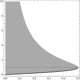
Figure 1: Plot associated with the combinatorial specification of binary trees where all nodes are counted, ${\mathcal{B}}=\mathcal{Z}+\mathcal{Z}\times\cramped{{\mathcal{B}}^{2}}$. The bottom thick black curve plots $C(z)=z+z\cramped{C(z)^{2}}$, or all coordinates $(z,C(z))$ usually considered for Boltzmann sampling; the shaded area is the region verifying $c\geqslant z+z\cramped{c^{2}}$, and from which we get coordinates $(z,c)$ which we use in our modified model.

Introduction

Being able to randomly generate large objects of any given combinatorial class (for instance described by a grammar), is a fundamental problem with countless applications in scientific modeling.

Nijenhuis and Wilf introduced the recursive method [16] in the late 70s (later extended by Flajolet et al. [12]), the first automatic random generation method; so termed automatic because it can directly derive random samplers from any combinatorial description—no bijection, no clever algorithm, no complicated equations are needed. The drawback is that this method is costly, notably in preprocessing: to compute the probabilities involved in generating an object of size $n$, the method requires knowing the complete enumeration of the combinatorial class up to size $n$; and predictably when $n$ is large, this enumeration is significant both to calculate and to store.

Enter Boltzmann sampling, introduced by Duchon et al. in 2002 [7, 8], of which the key insight was that a class’ enumeration is not required to compute the correct branching probabilities: instead, such probabilities can be obtained by evaluating the counting generating functions—for an unlabelled combinatorial class ${\mathcal{C}}$, for which there are $\cramped{c_{n}}$ elements of size $n$, its counting generating function is defined as

$$C(z):=\sum_{n=1}^{\infty}c_{n}z^{n}\text{.}$$

Through evaluation, all the coefficients of a generating function are smashed together, and the resulting probabilities take into account objects of all sizes. Thus, while you do know that the object returned will be uniformly sampled among objects of the same size, the size itself is a random variable—which you have no direct control over. As a result, a significant aspect of Boltzmann sampling involves: rejecting objects which are not within the desired size interval; manipulating the generating functions so the size distribution is such that not too many objects need be rejected.

The efficiency of this approach, combined with its mathematical appeal—in many regards Boltzmann sampling is an elegant and natural application of Analytic Combinatorics pioneered by Flajolet and Sedgewick [11]—have made it a fertile topic, and many of its aspects have been developed through a broad number of papers.

The Boltzmann model

A Boltzmann sampler for an unlabelled combinatorial class ${\mathcal{C}}$ (of which there are $\cramped{c_{n}}$ elements of size $n$), is an algorithm that draws any given object $\gamma\in{\mathcal{C}}$ with probability

$${\mathbb{P}}_{{z}}\!\left[{\gamma}\right]=\frac{z^{{\left|{\gamma}\right|}}}{C(z)}\qquad\text{with}\qquad C(z):=\sum_{n=1}^{\infty}c_{n}z^{n}\ =\sum_{\gamma\in{\mathcal{C}}}z^{{\left|{\gamma}\right|}}$$

where ${\left|{\gamma}\right|}$ denotes the size of object $\gamma$ and $z$ is some control parameter to be chosen. Thus the probability of obtaining an object of size $n$ is

$${\mathbb{P}}_{{z}}\!\left[{{\left|{\gamma}\right|}=n}\right]=\frac{c_{n}z^{n}}{C(z)}\qquad\qquad{\mathbb{P}}_{{s}}\!\left[{\gamma\ |\ {\left|{\gamma}\right|}=n}\right]=\frac{1}{c_{n}}$$

while the probability of drawing an object conditioned on its size is uniform.

The name of the method is an analogy to the Boltzmann model of statistical physics that assigns to each possible state of a system the probability $\cramped{\mathrm{e}^{-\beta E}/Z}$, where $E$ is the energy of the state, $\beta=1/T$ is a constant, and $Z$ is normalizing constant—the original authors noted that this was similar to the probability distribution of objects. But in truth, the distribution of the sizes of objects is a very generic distribution already known to probabilists as the Power Series Distribution, and according to Johnson et al. [13, §2.2], the terminology is usually credited to Noack [17] around 1950.

Evaluating GFs near their singularity

Boltzmann samplers depend on the evaluation of generating function in the neighborhood of their singularity—and it was assumed that this could be done in constant time arithmetic complexity.

The problem of how these functions should be evaluated was left open by the original paper, and remained without answer until the contribution of Pivoteau et al. [19, 20]. They introduced a variant of Newton’s iteration for combinatorial systems, which has a highly efficient quadratic convergence (and what’s more, is provably convergent for any specifiable combinatorial class). However some aspects have remained open:

1. Solving the evaluation problem does not entirely solve the issue of tuning the samplers—that is, picking the value of $z$, which will yield the best concentration of objects of the targeted size. Currently, expected value tuning requires inverting a system of equations, and to our knowledge this is not routinely done for large combinatorial systems. For certain combinatorial classes (algebraic classes), singular samplers are tuned by approaching the singularity as close as possible using a binary search, requiring making a logarithmic number of calls to the oracle, as shown by Darrasse [5].

2. As a related issue, it seems legitimate to ask: is evaluating the generating functions truly necessary, since these evaluations are in fine used to compute probabilities of average? and can relaxing this requirement possibly lead to more simple (or more efficient) implementations?

3. Finally, as a point of minor practical concern, but of conceptual interest: because of the finite nature of computers, and although the oracle can provide arbitrary precise values, the evaluation of generating functions is in practice restricted to fixed precision approximations. It has been argued that the incurred bias in uniformity is minimal: is it possible to make exact simulations from approximate values?

Our contribution: an extended framework.

This present paper attempts to investigate some of the aforementioned questions. Our novel idea appeals to the classical random generation concept of rejection, as described for instance in Devroye’s chapter on the rejection method [6, §2]. Instead of evaluating the generating functions exactly, we pick some nearby point that is easier to compute.

This is illustrated in Figure 1. Both Boltzmann samplers and our samplers use coordinates from the shaded region. But while Boltzmann samplers limit themselves to the coordinates that belong to the thick black curve at the bottom of the region, we allow ourselves to pick any point within the region. Of course, this introduces a bias, which needs to be compensated with some additional rejection. But we show that this rejection is constant and that for reasonable choices of coordinates it is practically negligible.

In this paper, we introduce this idea in Section 1, and showcase how it may be used through some illustrating examples: in Section 2, we show our samplers can enable using alternate techniques to determine the tuning parameter; in Section 3, we use the example of Otter trees (non plane binary trees) to show how we can circumvent having to make a non-constant number of evaluations of the generating function.

The ideas presented here followed from the first author’s work to extend Boltzmann samplers to infinite objects [2], and the second author’s attempts to modify generating functions to shape the size distribution of sampled objects.

Limits of this first version

This preliminary work comes with a set of restrictions: because none of the authors are presently familiar with the extensive litterature on multidimensional optimization, we have avoided describing how to apply this idea to combinatorial systems (or multitype definitions), focusing instead on combinatorial classes which can be described in a single equation. This is not because the idea of rejection cannot be trivially extended to systems, but rather because we felt this strengthened our exposition, while the added complexity (in notations, etc.) of describing systems could not be justified by our current findings.

1 Analytic Samplers

In this section, we provide the main definitions for our analytic random samplers, and then show the algorithms associated with the basic constructions.

We have used the name Analytic Samplers to distinguish our contribution in this paper from Boltzmann samplers, but it should be noted that the latter could legitimately be termed Analytic Samplers.

1.1 Main definitions

Definition 1.1

Let ${\mathcal{A}}$ be an unlabelled combinatorial class, and $a_{n}$ the number of objects from ${\mathcal{A}}$ that have size $n$. The ordinary generating function (OGF) associated with class ${\mathcal{A}}$ is defined equivalently by

$$A(z):=\sum_{n=0}^{\infty}a_{n}z^{n}\qquad\text{or}\qquad A(z):=\sum_{\alpha\in{\mathcal{A}}}z^{{\left|{\alpha}\right|}}\text{.}$$

The ordinary generating function enumerates combinatorial class it is associated to. The tenet of the symbolic method [11] is that if a combinatorial class can be symbolically specified using a set of operators (disjoint union, Cartesian product, sequence, multiset, etc.) from initial terminal symbols called atoms which have unit size, then this specification can be directly translated to obtain the ordinary generating function.

Definition 1.2

Let ${\mathcal{A}}$ be a symbolically defined combinatorial class which can be translated, following the symbolic method, to a functional equation on $A(z)$, the generating function associated with ${\mathcal{A}}$,

$${\mathcal{A}}=\Phi(\mathcal{Z},{\mathcal{A}},\mbox{\boldmath${\mathcal{X}}$})\qquad\Rightarrow\qquad A(z)=\phi(z,A(z),{\mbox{\boldmath$X$}}(z))\text{,}$$

where both $\Phi$ and $\phi$ may possibly involve other classes/generating functions which we note using vectors in bold (and each symbol/generating function component of the vector itself defined by their own equations).

Definition 1.3

Given a combinatorial class ${\mathcal{A}}$ as given in Definition 1.2, a pair of coordinates $(z,a)$ is said to be analytically valid coordinates for the combinatorial class ${\mathcal{A}}$ if and only if they verify the inequality

$$a\geqslant\phi(z,a,\mbox{\boldmath$x$})\text{.}$$

Remark. It is true that we could have some stronger bound, for instance, $a\geqslant A(z)$. But this is not desirable because the bound involves the generating function, the evaluation of which we are trying to avoid.

Indeed, a subtle remark is that while computing the right-hand side of the inequality is not necessary to run the analytic samplers, it is necessary to make the initial calibration. If this right-hand side depended on the generating function, we would be requiring strictly the same amount of work as traditional Boltzmann samplers—if not more!

In general, for convenience and clarity, we will omit the vector in the notations, and any additional bound symbols will be implicit.

Definition 1.4

An analytic sampler for an unlabelled combinatorial class ${\mathcal{A}}$ is an algorithm which samples an object $\alpha\in{\mathcal{A}}$, of size ${\left|{\alpha}\right|}$, with probability

$${\mathbb{P}}_{{(z,a)}}\!\left[{\alpha}\right]=\frac{z^{{\left|{\alpha}\right|}}}{a}$$

and fails with probability

$${\mathbb{P}}_{{(z,a)}}\!\left[{\mbox{\char 61}}\right]=1-\frac{A(z)}{a}$$

where $A(z)$ is the ordinary generating function associated with class ${\mathcal{A}}$, and the analytically valid coordinates $(z,a)$ are called the control parameter. Moreover we denote by $\cramped{\Gamma{\mathcal{A}}(\cramped{z,a})}$ such an analytic sampler.

Because the original Boltzmann samplers already used the concept of rejection to control the size of the output and constrain it to a tolerance interval, we choose instead to call our additional rejection, failure, to avoid confusion.

Theorem 1.1

Let ${\mathcal{A}}$ be a combinatorial class and $A(z)$ its generating function, and let $(z,a)$ be analytically valid coordinates for ${\mathcal{A}}$. The proportion of objects for which the generation has failed, does not depend on the size of the successfully generated object, and is equal to $1-A(z)/a$.

• This follows from the definition of the model of Analytic Samplers wherein the probability of a single draw failing is constant—in the sense that it does not depend on the size of the object that was being constructed when the sampling failed—and equal to

  $${\mathbb{P}}_{{(z,a)}}\!\left[{\mbox{\char 61}}\right]=1-\frac{A(z)}{a}\text{,}$$

  and thus an object (of some random size) is drawn with the complementary probability. The number of failures before an actual object is drawn is then geometrically distributed with $p=1-A(z)/a$. We then have:

  $${\mathbb{E}}_{{(z,a)}}\!\left[{\#\mbox{\char 61}}\right] =\sum_{k=0}^{\infty}k\left(1-\frac{A(z)}{a}\right)^{k}\frac{A(z)}{a}$$

  $$=\frac{A(z)}{a}\frac{\left(1-\frac{A(z)}{a}\right)}{\left(\frac{A(z)}{a}\right)^{2}}$$

  $$=\frac{a}{A(z)}\left(1-\frac{A(z)}{a}\right)=\frac{a}{A(z)}-1$$

  and because there is one last object generated (the one that does not fail, and after which we are done) the expected proportion of objects which have failed is ${\mathbb{E}}_{{(z,a)}}\!\left[{\#\mbox{\char 61}}\right]/({\mathbb{E}}_{{(z,a)}}\!\left[{\#\mbox{\char 61}}\right]+1)$ as stated.         

Note that the lower bound for $a$ is $a=A(z)$, and for this choice of value, the analytic sampler does not fail: the proportion of failed objects is 0%, and we revert to the case of Boltzmann samplers.

Indeed the inequality can naturally be seen as an equality involving a slack variable $\delta$, $a=\phi(z,a,\mbox{\boldmath$x$})+\delta$. In essence, if you are willing to spend the computational time needed to compute the generating function, then you are rewarded for your efforts by having no rejection at all.

1.2 Elementary constructions.

In this subsection, we give the basic constructions used by our analytic samplers. We follow the notation of the original article [8], and extend it to include our failure probability,

$$\Gamma{\mathcal{A}}:[p_{1}]\cdot\mathrm{Ber}\!\left({p_{2}}\right)\Rightarrow X\ |\ Y$$

means that we first fail with probability $1-p_{1}$, then we draw a Bernoulli variable $U$ of parameter $p_{2}$: if it is equal to $U=1$ then we return $X$, otherwise we return $Y$. Furthermore, when instead of a Bernoulli distribution, we have some variable $K$ drawn according to a discrete distrbution, we mean that we return a tuple of $K$ independent calls to the specified sampler.

Let ${\mathcal{A}}$, ${\mathcal{B}}$ and ${\mathcal{C}}$ be combinatorial classes. We recall, for clarity, that in this article we note ${\mathbb{P}}\!\left[{\alpha}\right]$ the probability of drawing an object $\alpha$; when we want to make explicit from which class this object is drawn, we note ${\mathbb{P}}\!\left[{\alpha\in{\mathcal{A}}}\right]$.

Disjoint union

Let ${\mathcal{A}}={\mathcal{B}}+{\mathcal{C}}$, and $a\geqslant b+c$. We first reject $1-(b+c)/a$ of the objects, then we do a normal Boltzmann.

$$\Gamma{\mathcal{A}}:\left[\frac{b+c}{a}\right]\cdot\mathrm{Ber}\!\left({\frac{b}{b+c}}\right)\Rightarrow\Gamma{\mathcal{B}}\ \ |\ \ \Gamma{\mathcal{C}}$$

• We must show that the sampler $\Gamma{\mathcal{A}}$ returns objects $\alpha\in{\mathcal{A}}$ with the correct probability ${\mathbb{P}}_{{(z,a)}}\!\left[{\alpha}\right]=z^{|\alpha|}/a$ (that is the probability of drawing an object from ${\mathcal{A}}$ follows the law given in Definition 1.4), assuming inductively that the generators $\Gamma{\mathcal{B}}$ and $\Gamma{\mathcal{C}}$ are correct.

  Hence:

  $$\begin{split}{\mathbb{P}}_{{(z,a)}}\!\left[{\alpha\in{\mathcal{A}}}\right]=\frac{b+c}{a}&\left(\frac{b}{b+c}{\mathbb{P}}_{{(z,b)}}\!\left[{\alpha\in{\mathcal{B}}}\right]\right.\\ &\left.+\,\frac{c}{b+c}{\mathbb{P}}_{{(z,c)}}\!\left[{\alpha\in{\mathcal{C}}}\right]\right)\end{split}$$

  that is, the probability of sampling an object from ${\mathcal{A}}$ is the probability of first not failing, $(b+c)/a$, and then the probability of drawing the object using the sampler for class ${\mathcal{B}}$ or ${\mathcal{C}}$ with the correct Bernoulli probability. By hypothesis those two samplers return objects with correct probabilities, so

  $${\mathbb{P}}_{{(z,a)}}\!\left[{\alpha\in{\mathcal{A}}}\right] =\frac{b+c}{a}\left(\frac{b}{b+c}\frac{z^{|\alpha|}}{b}+\frac{c}{b+c}\frac{z^{|\alpha|}}{c}\right)=\frac{z^{|\alpha|}}{a}\text{.}$$

  Note that in this proof, and the following, we do not explicitly prove the probability of failure as it is a straightforward consequence: sum the probability of drawing an object over all possible possible objects, and take the complimentary probability.         

Cartesian product

Let ${\mathcal{A}}={\mathcal{B}}\times{\mathcal{C}}$, and $a\geqslant b\cdot c$.

$$\Gamma{\mathcal{A}}:\left[\frac{b\cdot c}{a}\right]\Rightarrow\left(\Gamma{\mathcal{B}}\ \ ;\ \ \Gamma{\mathcal{C}}\right)$$

• The proof follows the same model as the previous construction; let $\alpha=(\beta,\gamma)$,

  $${\mathbb{P}}_{{(z,a)}}\!\left[{\alpha\in{\mathcal{A}}}\right] =\frac{b\cdot c}{a}{\mathbb{P}}_{{(z,b)}}\!\left[{\beta\in{\mathcal{B}}}\right]{\mathbb{P}}_{{(z,c)}}\!\left[{\gamma\in{\mathcal{C}}}\right]$$

  and since the samplers for $\Gamma{\mathcal{B}}$ and $\Gamma{\mathcal{C}}$ are inductively assumed to be correct,

  $${\mathbb{P}}_{{(z,a)}}\!\left[{\alpha\in{\mathcal{A}}}\right] =\frac{b\cdot c}{a}\frac{z^{|\beta|}}{b}\frac{z^{|\gamma|}}{c}=\frac{z^{|\beta|+|\gamma|}}{a}=\frac{z^{|\alpha|}}{a}\text{.}$$

          

Example. At this point we will illustrate the initial definitions and these constructors by looking at the class ${\mathcal{B}}$ of binary trees, in which all nodes both internal and external count towards the size of the tree. These trees can be symbolically specified as either a leaf ($\mathcal{Z}$) or a node which has two subtrees ($\mathcal{Z}\times\cramped{{\mathcal{B}}^{2}}$),

(1.1) $${\mathcal{B}}=\mathcal{Z}+\mathcal{Z}\times{\mathcal{B}}^{2}\quad\Rightarrow\quad B(z)=z+zB(z)^{2}\text{.}$$

This functional equation can then be translated to an inequality,

$$b\geqslant z+zb^{2}\text{.}$$

The analytically valid coordinates for ${\mathcal{B}}$ are all points that belong to the shaded region in Figure 1. The corresponding analytic sampler is:

$$\Gamma{\mathcal{B}}:\left[\frac{z+zb^{2}}{b}\right]\cdot\mathrm{Ber}\!\left({\frac{z}{z+zb^{2}}}\right)\Rightarrow\blacksquare\ \ |\ \ \left(\Gamma{\mathcal{B}}\ \ ;\ \ \Gamma{\mathcal{B}}\right)$$

where $\blacksquare$ is a leaf of unit weight.

Sequence

Let ${\mathcal{A}}={\text{\sc Seq}}\left({\mathcal{B}}\right)$ and $a\geqslant 1/(1-b)$.

$$\Gamma{\mathcal{A}}:\left[\frac{(1-b)^{-1}}{a}\right]\cdot\mathrm{Geo}\!\left({b}\right)\Rightarrow\left(\Gamma{\mathcal{B}},\ldots\right)$$

• We follow again the same model as previously. Let $\alpha=(\beta_{1},\ldots,\beta_{k})$.

  $${\mathbb{P}}_{{(z,a)}}\!\left[{\alpha\in{\mathcal{A}}}\right]=\frac{(1-b)^{-1}}{a}{\mathbb{P}}\!\left[{\mathrm{Geo}\!\left({b}\right)=k}\right]\prod_{i=1}^{k}{\mathbb{P}}_{{(z,b)}}\!\left[{\beta_{i}\in{\mathcal{B}}}\right]$$

  and by hypothesis

  $${\mathbb{P}}_{{(z,a)}}\!\left[{\alpha\in{\mathcal{A}}}\right] =\frac{(1-b)^{-1}}{a}{b}^{k}(1-b)\prod_{i=1}^{k}\frac{z^{|\beta_{i}|}}{b}$$

  $$=\frac{(1-b)^{-1}}{a}{b}^{k}(1-b)\frac{z^{|\beta_{1}|+\ldots+|\beta_{k}|}}{{b}^{k}}$$

  $$=\frac{z^{|\beta_{1}|+\ldots+|\beta_{k}|}}{a}=\frac{z^{|\alpha|}}{a}\text{.}$$

          

1.3 Illustration of the rate of failure with Cayley Trees.

For the purpose of giving an example that is somewhat more interesting than binary trees, we go slightly beyond the scope of unlabelled constructions which we have presented thus far, and present a labelled class which uses the Set operator. The point of this subsection is to illustrate, with an example, how moving away from the curve of a generating function impacts the rate of failure—that is, the rejection which must be done to compensate for sampling bias introduced by the approximation.

Consider the example given by the class ${\mathcal{T}}$ of Cayley trees (labelled, unrestricted, non-plane trees), symbolically specified as ${\mathcal{T}}=\mathcal{Z}\star{\text{\sc Set}}\left({\mathcal{T}}\right)$. The exponential generating function of this class, $T(z)=z\cramped{\mathrm{e}^{T(z)}}$, is closely related to Lambert’s $W$-function, which is implicitly defined. Actual standalone implementations of Boltzmann samplers requiring this function have, for instance, have resorted to using its truncated Taylor series expansion, see Bassino et al. [1].

  

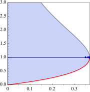
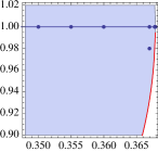
Figure 2: This is a plot of the region defined by the inequality $t\geqslant z\cdot\cramped{\exp{\left({t}\right)}}$, with $z$ on the $x$-axis and $t$ on the $y$-axis. The lower bound of the region, in bolded-red, is the curve of the exponential generating function $T(z)$. Each point corresponds to one of the columns of Table 1. The second figure, on the right, is a close-up near the singularity, at $z=\cramped{\mathrm{e}^{-1}}$.

With analytic samplers, our starting point is the system of functional equations yielded by the symbolic method (here there is only a single equation), replace any occurrence of a function by a free variable, and obtain the inequality $t\geqslant z\cdot\cramped{\exp{\left({t}\right)}}$ and the algorithm

$$\Gamma{\mathcal{T}}(z,t):\left[\frac{z\exp{\left({t}\right)}}{t}\right]\cdot\mathrm{Poi}\!\left({t}\right)\Rightarrow\square(\Gamma{\mathcal{T}}(z,t),\ldots,\Gamma{\mathcal{T}}(z,t))$$

in other words, after an initial rejection (what we call failure) with probability $z\cdot\cramped{\exp{\left({t}\right)}}/t$ to account for the approximation of the generating function, we draw a Poisson random variable of parameter $t$, to indicate how many children to generate.

It is straightforward enough to see that this algorithm is correct for any pair $(z,t)$ which satisfies the aforementioned inequality. Notice also the failure ratio can easily be simulated exactly using techniques described by Flajolet et al. [10].

An experiment summarized in Table 1 illustrates that the impact of approximation is modest. For various pairs of $(z,t)$, the table summarizes the result of making 1000 calls to the sampler: it indicates in what proportion the sampling failed prematurely; and makes note of the average and maximal size among the trees actually drawn. The case where $z=\cramped{\mathrm{e}^{-1}}$ and $t=1=T(z)$ is special: first because this is the only case in which $t$ is exactly equal to the evaluated EGF (thus we have $0\%$ failure and our analytic sampler is a traditional Boltzmann sampler); second because since we are evaluating the EGF in its singularity, this is actual a singular Boltzmann sampler (for which the expected value of the size of the output in unbounded). All other points, as illustrated in Figure 2 are more or less distant to the plot of $T(z)$, with a consequently higher failure rate: but even at relatively significant distance from the curve, the failure rate remains largely tolerable.

• 	$t=1$							$t=0.98$
  $z\;\;=$	0.35	0.36	0.367	0.3678	0.36787	0.367879	$\mathrm{e}^{-1}$	0.367
  failure (observed)	28.8%	19.2%	6.4%	1.7%	0.4%	0.3%	0%	3.5%
  failure (theoretical)	28.3%	19.4%	6.8%	2.1%	0.7%	0.2%	0%	3.9%
  average size	6.6	9.9	28.8	127.	177.3	2716.7	4944.3	35.9
  maximal size	235	131	1493	17 799	26 531	826 167	2 518 975	1563

Table 1: This table summarizes the result of making 1000 calls to an analytic sampler for Cayley trees, with various values of $z$ (the control parameter) and $t$ (the approximation of the generating function). The failure is the ratio of trees that must be rejected as a direct result of approximating the generating function, instead of evaluating it. Thus for the pair of values $z=\cramped{\mathrm{e}^{-1}}$ and $t=1=T(z)$, in which we use the exact value of $T(z)$, our samplers are exactly equivalent to Boltzmann samplers, hence the failure is of $0\%$. What is remarkable is that the failure resulting from rather large approximations remains manageable.

2 Simply generated trees

We now would like to illustrate how dealing with a region (and inequality) might make searching for an optimal pair of values for the sampler easier. It this section, we show how we can search for the best value of the tuning parameter $z$ (which happens to be in the vicinity of the singularity) for a family of combinatorial classes, without evaluating the generating function a logarithmic number of times.

Simply generated trees were introduced by Meir and Moon [15] as classes of trees defined by the following specification

(2.2) $${\mathcal{Y}}=\mathcal{Z}\times\Phi({\mathcal{Y}})$$

where $\Phi$ is a polynomial defined as

(2.3) $$\Phi(x)=\sum_{\omega\in\Omega}x^{\omega}\qquad\Phi(x)=\sum_{\omega\in\Omega}\frac{x^{\left|\omega\right|}}{{\left|\omega\right|}!}$$

respectively depending on whether the class is unlabelled or labelled, and where $\Omega\subseteq{{\mathbb{N}}}$ is the multiset of allowable degrees (for instance, for binary trees, $\Omega=\left\{0,2\right\}$). Meir and Moon identified that trees families defined in such a way shared an important number of common properties (such as mean path length of order $n\sqrt{n}$ or average height of order $\sqrt{n}$).

2.1 Existing approaches.

Randomly sampling from this class of tree is no longer particularly challenging: there are several methods to do this, with various properties of optimality (time, random-bit, etc.). So we do not presume to introduce samplers with any sort of new efficiency. However the example of simply generated trees illustrates a way in which calibration might be more practical with analytic samplers.

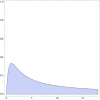
Figure 3: This is the plot of a the generating function of a simply generated tree (in this case, the class ${\mathcal{U}}$ of unary-binary trees, i.e., $\Omega=\left\{0,1,2\right\}$). On the left, the $x$-axis is $z$, the control parameter and the $y$-axis has $U(z)=z\Phi(U(z))$. On the right, we are plotting the function $u\mapsto u/\Phi(u)$. The problem of looking for the singularity, left, has been reduced to the more palatable problem of maximizing a function, right.

Simply generated trees happen to have a branching singularity. This means: that their generating function can be evaluated at the singularity, and also that the size distribution of objects produced by a Boltzmann sampler would be ‘peaked’, that is, highly concentrated towards smaller objects. The solution has traditionally been to do singular sampling: to pick $z$ as being at, or near, the singularity, generate objects with unbounded expected size, and reject those that are too big.

Except in simple cases (such as binary trees, for which the singularity is well known to be $1/4$), the singularity is not known, so it must be determined empirically. This is usually done with a binary search, as implemented by Darrasse [5]: the oracle introduced by Pivoteau et al. [20] converges when inside the radius of convergence, and diverges otherwise; thus it is possible to detect whether we have gone beyond the singularity. This method requires a logarithmic number of calls to the oracle—a logarithmic number of evaluations that are not done in constant time.

2.2 New approach: maximize a polynomial.

From the specification in Equation 2.2, we obtain the condition for analytic-validity of a pair $(z,y)$,

$$y\geqslant z\cdot\Phi(y)\text{.}$$

With this, it is now easier, instead of looking at the generating function $Y(z)$, to look instead at $y\mapsto y/\Phi(y)$, which is a rational function. This function admits a maximal point in the unit interval, which is the singular point of $Y(z)$.

Looking for this maximal point is a considerably easier problem, that does not require any evaluation of the generating function (except perhaps for an initial guess): it can be solved by differentiation, by Newton iteration, or with specifically optimized algorithms available in the litterature, such as Brent’s algorithm [4].

3 Substitution operator

While we have only described, for space and pertinence purposes, how to build analytic samplers for classes using elementary constructors, the possibilities are much broader. In particular, functional operators, such as pointing (differentiation) or substituting (composition) can naturally be used.

We will not go into detail, but instead provide the example of the unordered pair, $\cramped{{\text{\sc MSet}}_{2}}$, and present an application with the random sampling of Otter trees.

3.1 Unordered pair construction

Let ${\mathcal{B}}$ be a combinatorial class, and ${\mathcal{A}}={\text{\sc MSet}}_{2}\left({\mathcal{B}}\right)$ be the class containing unordered pairs of elements of ${\mathcal{B}}$. The corresponding generating functions $A(z)$ and $B(z)$ verify the functional equation

$$A(z)=\frac{B(z)^{2}+B(\cramped{z^{2}})}{2}\text{.}$$

Assuming there is an analytic sampler for ${\mathcal{B}}$, we can build an analytic sampler for ${\mathcal{A}}$. Let $(z,b)$ and $(\cramped{z^{2}},\bar{b})$ both be analytically valid for ${\mathcal{B}}$ (note that the variable $z$ must be the same in both pairs), and let $(z,a)$ be analytically valid for ${\mathcal{A}}$, that is

$$a\geqslant\frac{b^{2}+\bar{b}}{2}\text{.}$$

Using the notation we have introduced,

$$\begin{split}\cramped{\Gamma{\mathcal{A}}(\cramped{z,a})}:\left[\frac{b^{2}+\bar{b}}{2a}\right]\cdot\ &\mathrm{Ber}\!\left({\frac{b^{2}}{b^{2}+\bar{b}}}\right)\Rightarrow\\ &\left\{\cramped{\Gamma{\mathcal{B}}(\cramped{z,b})}\ ;\ \cramped{\Gamma{\mathcal{B}}(\cramped{z,b})}\right\}\ \ |\\ &\cramped{\Gamma{\mathcal{B}}(\cramped{z^{2},\bar{b}})}\text{ and duplicate}\text{.}\end{split}$$

In other terms, after making the obligatory failure test, we choose with the proper probability whether to create a pair of elements resulting from independent calls to $\cramped{\Gamma{\mathcal{B}}(\cramped{z,b})}$, or whether to make one call to $\cramped{\Gamma{\mathcal{B}}(\cramped{\cramped{z^{2}},\bar{b}})}$ and duplicating the resulting object to make a pair of identical objects.

• As before, proving the validity of this algorithm involves showing that the analytic sampler $\cramped{\Gamma{\mathcal{A}}(\cramped{z,a})}$ returns any object $\alpha\in{\mathcal{A}}$ with probability $\cramped{z^{{\left|{\alpha}\right|}}}/a$. We distinguish two disjoint cases.

  • Either the pair $\alpha=\left\{\cramped{\beta_{1}};\cramped{\beta_{2}}\right\}$ contains two distinct elements, $\cramped{\beta_{1}}\not=\cramped{\beta_{2}}$. Then this pair could only have been produced by two independent (and distinguished) calls to $\cramped{\Gamma{\mathcal{B}}(\cramped{z,b})}$. Thus under this setting,

    $$\begin{split}{\mathbb{P}}_{{z,a}}\!\left[{\alpha\ |\ \beta_{1}\not=\beta_{2}}\right]=\frac{b^{2}+\bar{b}}{2a}&\cdot\frac{b^{2}}{b^{2}+\bar{b}}\cdot\\ &\left({\mathbb{P}}_{{z,b}}\!\left[{\beta_{1}}\right]\cdot{\mathbb{P}}_{{z,b}}\!\left[{\beta_{2}}\right]\right.\\ &\left.+\,{\mathbb{P}}_{{z,b}}\!\left[{\beta_{2}}\right]\cdot{\mathbb{P}}_{{z,b}}\!\left[{\beta_{1}}\right]\right)\text{.}\end{split}$$

    By hypothesis, $\cramped{\Gamma{\mathcal{B}}(\cramped{z,b})}$ is an analytic sampler for class ${\mathcal{B}}$, which means it returns an object $\beta\in{\mathcal{B}}$ with probability $\cramped{z^{{\left|{\beta}\right|}}}/b$,

    $${\mathbb{P}}_{{z,a}}\!\left[{\alpha\ |\ \beta_{1}\not=\beta_{2}}\right] =\frac{b^{2}+\bar{b}}{2a}\cdot\frac{b^{2}}{b^{2}+\bar{b}}\frac{2z^{{\left|{\beta_{1}}\right|}+{\left|{\beta_{2}}\right|}}}{b^{2}}$$

    $$=\frac{z^{{\left|{\beta_{1}}\right|}+{\left|{\beta_{2}}\right|}}}{a}=\frac{z^{{\left|{\alpha}\right|}}}{a}\text{.}$$

  • Or the pair $\alpha=\left\{\beta;\beta\right\}$ contains two identical objects. The pair could then have been drawn by either branch: from two independent calls to $\cramped{\Gamma{\mathcal{B}}(\cramped{z,b})}$ which happen to return the same object; or from the call to $\cramped{\Gamma{\mathcal{B}}(\cramped{z^{2},\bar{b}})}$ which is duplicated. In this case,

    $$\begin{split}{\mathbb{P}}_{{z,a}}\!\left[{\alpha\ |\ \beta=\beta}\right]=\frac{b^{2}+\bar{b}}{2a}\cdot&\left(\frac{b^{2}}{b^{2}+\bar{b}}\cdot{\mathbb{P}}_{{z,b}}\!\left[{\beta}\right]^{2}\right.\\ &\left.+\,\frac{b^{2}}{b^{2}+\bar{b}}\cdot{\mathbb{P}}_{{\cramped{z^{2}},\bar{b}}}\!\left[{\beta}\right]\right)\text{.}\end{split}$$

    Assuming the analytic sampler for ${\mathcal{B}}$ is correct,

    $$\begin{split}{\mathbb{P}}_{{z,a}}\!\left[{\alpha\ |\ \beta=\beta}\right]&=\frac{b^{2}+\bar{b}}{2a}\cdot\left(\frac{b^{2}}{b^{2}+\bar{b}}\cdot\left(\frac{z^{{\left|{\beta}\right|}}}{b}\right)^{2}\right.\\ &\phantom{=\frac{b^{2}+\bar{b}}{2a}\cdot\quad}\left.+\,\frac{b^{2}}{b^{2}+\bar{b}}\cdot\frac{(\cramped{z^{2}})^{{\left|{\beta}\right|}}}{\bar{b}}\right)\end{split}$$

    which finally yields

    $${\mathbb{P}}_{{z,a}}\!\left[{\alpha\ |\ \beta=\beta}\right] =\frac{z^{2{\left|{\beta}\right|}}}{a}=\frac{z^{{\left|{\alpha}\right|}}}{a}\text{.}$$

          

3.2 Otter Trees

We’ve already thoroughly discussed the class ${\mathcal{B}}$ of binary trees. These binary trees are plane, in the sense that there the children of an internal node are distinguished: there is a left node and a right node. We now consider the class ${\mathcal{V}}$ of Otter tree, which are binary trees that are non plane, using the $\cramped{{\text{\sc MSet}}_{2}}$ operator introduced in the previous subsection,

$${\mathcal{V}}=\mathcal{Z}+{\text{\sc MSet}}_{2}\left({\mathcal{V}}\right)\text{.}$$

The generating function $V(z)$ for Otter trees satisfies the functional equation

$$V(z)=z+\frac{V(z)^{2}+V(\cramped{z^{2}})}{2}\text{,}$$

and note that, for this class, we only count external nodes. This combinatorial class does not have a closed form generating function: prior Boltzmann samplers for Otter trees have already informally used approximations [9, §5]; Pivoteau [18] used the fact that $V(z)=1-\sqrt{1-2z-V(\cramped{z^{2}})}$. In practice these approximations yield correct simulations, but theoretically they could introduce a bias. With analytic samplers, this possible bias is corrected by failing with some probability; this also gives us more flexibility to choose the approximations.

•   

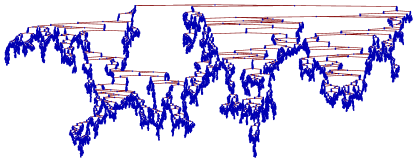
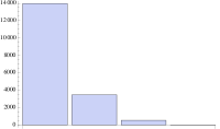
Figure 4: An Otter tree of size $n=17\,979$ (we were targeting $20\,000\pm 10\%$), generated in $13s$ on a standard 2012 laptop computer. The bar chart summarizes the degree of symmetry of the leaves: the first bar indicates how many leaves are not duplicated; then duplicated once; then four times; then eight times.

Setting up the inequality

For our analytical samplers, we need the values $\cramped{v_{[i]}}$, corresponding to $V(\cramped{z^{2^{i}}})$, which are defined recursively by the system of inequalities

(3.4) $$\forall i\in\mathbb{N}^{+},\quad v_{[i]}\geqslant z^{2^{i}}+\frac{{v_{[i]}}^{2}+v_{[i+1]}}{2}\text{.}$$

Because this system is infinite, we are first going to pick a threshold index after which the equations will be approximated; and we will determine a good approximation for the remaining terms.

In order to find solutions, we need an initial interval for $z$, which need not be especially precise: to this end, $0\leqslant z\leqslant 1$ suffices (even though it is simple enough to argue that $1/4<z<1/2$). The constant part of this recursive inequation is $\cramped{z^{2^{i}}}$, thus it makes sense to let $\cramped{v_{[i]}}=K\cramped{z^{2^{i}}}$, which we can then inject in our inequation. Dividing both sides by $\cramped{z^{2^{i}}}$ and factoring, we obtain

(3.5) $$K\geqslant 1+\frac{Kz^{2^{i}}}{2}\left(K+1\right)\text{.}$$

Choosing parameters

At this point we now have two parameters to pick. First we have to find a constant $K$ satisfying Inequation (3.5); $K$ can be as small as we want, as long as $K>1$.

Once we have picked a threshold $\cramped{i_{0}}$, and the constant $K$ which will approximate terms $\cramped{v_{[i]}}$ for $i>i_{0}$, we can exactly compute the initial terms. This is done by solving exactly the quadratic equations,

$$\frac{1}{2}{v_{[i]}}^{2}-v_{[i]}+\left(z^{2^{i}}+\frac{1}{2}v_{[i+1]}\right)=0$$

going backwards from $\cramped{i_{0}}-1$ to $0$, and with, as we said, the remaining terms $\cramped{o_{[i]}}=K\cramped{z^{2^{i}}}$.

The approximations we have taken here will impact the failure rate, and we can decrease it by taking any of the following measures: we can pick a higher threshold $\cramped{i_{0}}$; we can pick a $z$ that is closer to the singularity; we can use more than the constant part of the equation in the step where we reject $\cramped{z^{2^{i+1}}}$ to approximate the terms beyond the threshold.

This leads to an efficient sampler for Otter trees, of which we have drawn a very large tree in Figure 4. Consider that this allows for interesting empirical analyses of these trees.

4 Conclusion

In this paper, we have proposed to integrate the classical idea of rejection sampling to the Boltzmann sampler model, therefore relaxing the condition that generating functions must be evaluated exactly.

The resulting model, which we call analytic samplers, is fully compatible with all prior approaches used in Boltzmann samplers (in particular, these samplers can work well with Pivoteau et al.’s oracle), and in fact provides sound theoretical ground by which to allow the routine approximations that have been made in existing Boltzmann samplers.

But beyond that, we also believe the relaxed properties can allow for possible improvements and simplifications in the way the samplers target the size of their output. To illustrate these ideas, we show two types of applications. First, with the example of simply generated trees, we illustrate how tuning can be done in an alternate way, by using the added degree of freedom of exploring points in a region instead of a curve. Second, we show for Otter trees, that our samplers allow for much larger approximation to be made with little side-effects.

Some details involve how to simulate the probabilities without resorting to arbitrary precision: several answers exist, for instance in the form of Buffon machine as introduced by Flajolet et al. [10] or, because we are not restricted to fixed curve, selecting only rational probabilities, which can be easily simulated exactly, as shown by Lumbroso [14].

The open question is to determine whether these properties can be leveraged for large combinatorial systems: indeed, the initial Boltzmann paper was only illustrated by combinatorial classes defined as one or a handful of equations. The real impressive strength of the oracle provided by Pivoteau et al. [20] was to be able to handle combinatorial systems with thousands of equations. It remains to be seen if, when dealing with much more complex polytopes, it is possible to use simple refinements of the ideas we have shown for simply generated trees. Finally, an topic which has not yet reached practical maturity is that of multidimensional combinatorial classes (where the distribution is not uniform, but biased according to some combinatorial parameter). The article of Bodini and Ponty [3] has highlighted some issues, which we believe our present framework might help bypass.

References

- [1] Frédérique Bassino, Julien David, and Cyril Nicaud. Regal: A library to randomly and exhaustively generate automata. In Jan Holub and Jan Žďárek, editors, Implementation and Application of Automata, volume 4783 of Lecture Notes in Computer Science, pages 303–305. Springer Berlin Heidelberg, 2007.
- [2] Olivier Bodini, Guillaume Moroz, and Hanane Tafat-Bouzid. Infinite Boltzmann samplers and applications to branching processes. In Proceedings of GASCOM 2012, pages 1–7, June 2012.
- [3] Olivier Bodini and Yann Ponty. Multi-dimensional Boltzmann sampling of languages. DMTCS Proceedings, 0(01):49–64, 2010.
- [4] Richard P. Brent. Algorithms for minimization without derivatives. Courier Dover Publications, 1973.
- [5] Alexis Darrasse. Structures arborescentes complexes: analyse combinatoire, génération aléatoire et applications. PhD thesis, Paris 6, 2010.
- [6] Luc Devroye. Non-Uniform Random Variate Generation. Springer Verlag, 1986.
- [7] Philippe Duchon, Philippe Flajolet, Guy Louchard, and Gilles Schaeffer. Random sampling from Boltzmann principles. In Peter Widmayer et al., editor, Automata, Languages, and Programming, number 2380 in Lecture Notes in Computer Science, pages 501–513. Springer Verlag, 2002.
- [8] Philippe Duchon, Philippe Flajolet, Guy Louchard, and Gilles Schaeffer. Boltzmann samplers for the random generation of combinatorial structures. Combinatorics, Probability and Computing, 13(4–5):577–625, 2004. Special issue on Analysis of Algorithms.
- [9] Philippe Flajolet, Éric Fusy, and Carine Pivoteau. Boltzmann sampling of unlabelled structures. In David Applegate et al., editor, Proceedings of the Ninth Workshop on Algorithm Engineering and Experiments and the Fourth Workshop on Analytic Algorithmics and Combinatorics, pages 201–211. SIAM Press, 2007. Proceedings of the New Orleans Conference.
- [10] Philippe Flajolet, Maryse Pelletier, and Michèle Soria. On Buffon machines and numbers. In Dana Randall, editor, Proceedings of the Twenty-Second Annual ACM-SIAM Symposium on Discrete Algorithms, SODA 2011, pages 172–183. SIAM, 2011.
- [11] Philippe Flajolet and Robert Sedgewick. Analytic Combinatorics. Cambridge University Press, 2009. 824 pages (ISBN-13: 9780521898065); also available electronically from the authors’ home pages.
- [12] Philippe Flajolet, Paul Zimmerman, and Bernard Van Cutsem. A calculus for the random generation of labelled combinatorial structures. Theoretical Computer Science, 132(1-2):1–35, 1994.
- [13] Norman L. Johnson, Adrienne W. Kemp, and Samuel Kotz. Univariate Discrete Distributions. Wiley Series in Probability and Statistics. John Wiley & Sons, Inc., 3rd edition, 2005.
- [14] Jérémie Lumbroso. Optimal Discrete Uniform Generation from Coin Flips, and Applications. Preprint, 2013.
- [15] A. Meir and J. W. Moon. On the altitude of nodes in random trees. Canadian Journal of Mathematics, 30:997–1015, 1978.
- [16] Albert Nijenhuis and Herbert S. Wilf. Combinatorial Algorithms. Academic Press, 2nd edition, 1978.
- [17] Albert Noack. A Class of Random Variables with Discrete Distributions. The Annals of Mathematical Statistics, 21(1):127–132, March 1950.
- [18] Carine Pivoteau. Mémoire de master d’informatique. génération aléatoire et modeles de boltzmann. Master’s thesis, 2009.
- [19] Carine Pivoteau, Bruno Salvy, and Michèle Soria. Boltzmann oracle for combinatorial systems. In Proceedings of the Fifth Colloquium on Mathematics and Computer Science. Blaubeuren, Germany, pages 475–488, 2008.
- [20] Carine Pivoteau, Bruno Salvy, and Michèle Soria. Algorithms for combinatorial structures: Well-founded systems and Newton iterations. Journal of Combinatorial Theory, Series A, 119(8):1711–1773, 2012.