Period Error Estimation for the Kepler Eclipsing Binary Catalog

Abstract

The Kepler Eclipsing Binary Catalog (KEBC) describes 2165 eclipsing binaries identified in the 115 deg² Kepler Field based on observations from Kepler quarters Q0, Q1, and Q2. The periods in the KEBC are given in units of days out to six decimal places but no period errors are provided. We present the PEC (P eriod E rror C alculator) algorithm which can be used to estimate the period errors of strictly periodic variables observed by the Kepler Mission. The PEC algorithm is based on propagation of error theory and assumes that observation of every light curve peak/minimum in a long time-series observation can be unambiguously identified. The PEC algorithm can be efficiently programmed using just a few lines of C computer language code. The PEC algorithm was used to develop a simple model which provides period error estimates for eclipsing binaries in the KEBC with periods less than 62.5 days: $\log\sigma_{P}\approx{-5.8908+1.4425\!\left(1+\log P\right)}$, where $P$ is the period of an eclipsing binary in the KEBC in units of days. KEBC systems with periods $\geq$62.5 days have KEBC period errors of $\sim$0.0144 days. Periods and period errors of 7 eclipsing binary systems in the KEBC were measured using the NASA Exoplanet Archive Periodogram Service and compared to period errors estimated using the PEC algorithm.

1 INTRODUCTION

Prša et al. (2011) produced the Kepler Eclipsing Binary Catalog (KEBC) which contained 1879 unique eclipsing and ellipsoidal binary systems identified in the 115 deg² Kepler Field using the first Kepler data release (Borucki et al., 2011, and references therein) which covered the first 44 days of the operation of the Kepler Mission (Kepler quarters Q0 and Q1). For each object (binary system), the KEBC provides the Kepler ID (KID) number, the period, $P_{0}$, the ephemeris zero point, BJD₀, morphology type, and various physical parameters from the Kepler Input Catalog. For detached and semi-detached eclipsing binary systems, the KEBC provides the several principal parameters including the temperature ratio of the two stars, $T_{2}/T_{1}$, the sum of the fractional radii, $\rho_{1}+\rho_{2}$, the radial and tangential components of the eccentricity, $e\sin(\omega)$ and $e\cos(\omega)$, and the sine of the inclination, $\sin(i)$. For overcontact systems, the KEBC provides $T_{2}/T_{1}$, the photometric mass ratio $q$, the fillout factor, and $\sin(i)$.

Slawson et al. (2011) updated the Kepler Eclipsing Binary Catalog by increasing the baseline nearly fourfold to 125 days by including the second Kepler data release (Kepler quarter Q2). Three hundred and eighty-six new systems were added, and the ephemerides (BJD₀ and $P_{0}$) and principle parameters were recomputed. This version of the KEBC contained 2165 objects which is 1.4% of all Kepler target stars.

The online version of the Kepler Eclipsing Binary Catalog is hosted at Villinova University. The current online version of the KEBC (as of 2013 January 22: Revision 1.96, 2011-06-15) has information on 2176 systems. The online version includes figures for each object showing the raw Kepler light curve, the detrended light curve, and the phased light curve with a polynomial model “fit” to the data, as determined by the same neural network analysis which produced the principal parameters.

The statistical properties of the Kepler Eclipsing Binary Catalog were determined using the EBAI method (E clipsing B inaries via Artificial I ntelligence; Prša et al. 2008). The EBAI method uses several trained neural networks to determine the principal parameters for every binary system in the KEBC. The performance of EBAI on detached eclipsing binaries is described in §4.2.2. of Prša et al. (2011); Figure 10 shows the performance of EBAI method on a test set of 10,000 detached eclipsing binaries for 5 parameters: $\sin(i)$, $e\sin(\omega)$, $e\cos(\omega)$, $\rho_{1}+\rho_{2}$, and $T_{1}/T_{2}$. It was determined that 90% of all systems had errors smaller than 10% in all 5 parameters. Unfortunately, no error analysis was provided for the periods determined using the test set of 10,000 detached eclipsing binaries.

The periods in the Kepler Eclipsing Binary Catalog are given in units of days out to six decimal places. One microday is 86.4 milliseconds (ms). As shown below, the periods for many of KEBC binary systems must have measurement errors that are significantly greater than 86.4 ms — especially for the systems that had only a few complete cycles (periods) in 125 days. Although no error analysis has been provided for the periods given in the KEBC, we show below that it is possible to determine reasonable error estimates for periods given in the KEBC ex post facto without the need to reanalyze the original Kepler light curves.

This article describes how the period errors of strictly periodic variables observed by the Kepler Mission can be estimated using the new PEC (P eriod E rror C alculator) algorithm which is based on propagation of error theory. The PEC algorithm is described in the next section. The PEC algorithm is used in §3 to estimate the period errors for periods ranging from 0.1 to 125 days of the 2176 binary systems in the Kepler Eclipsing Binary Catalog. These theoretical predictions are then compared with measured period errors from Kepler observations of five detached and two semi-detached eclipsing binary systems in the KEBC. The article concludes in §4 with a brief discussion of the limitations of using the PEC algorithm with observations of strictly periodic variables with morphologically complicated light curves like RR Lyraes.

2 PERIOD ERROR ESTIMATION

In this section we investigate period errors as determined with propagation of error theory of 10-day uninterrupted time series observations of strictly periodic variables with periods of 7.3 days, 4.7 days, and 2.4 days. These results are summarized in the last subsection which describes the PEC algorithm that can be used to estimate the period errors in the Kepler Eclipsing Binary Catalog.

2.1 One Cycle

Let us start with a simple example. Consider a 10-day time series of uninterrupted space-based 30-min observations of a periodic variable with a period $P\!=\!7.3$ days and a timing uncertainty of $\sigma\!=\!0.0104$ days (one-half bin width: 15 min). For the sake of simplicity, assume that the first peak flux of the light curve occurs during the first observation. Only a single measurement of a single period is possible. There will be two peak flux values at $t_{1}$ and $t_{2}$. The estimated period is

$$P_{1}=t_{2}-t_{1}\,,$$ (1)

and the variance of $P_{1}$ is

$$\sigma^{2}_{P_{1}}=\sigma_{t_{2}}^{2}+\sigma_{t_{1}}^{2}=2\,\sigma^{2}\,,$$ (2)

using propagation of error theory (e.g., Bevington, 1969). The uncertainty of the period is

$$\sigma_{P_{1}}=\sqrt{2}\,\sigma\,,$$ (3)

which is 0.0147 days (21.2 min).

This example used the maximum integrated flux value as the key feature to be identified in each cycle (period) of the light curve. This is, of course, an arbitrary choice. One could instead choose any other unique feature of the light curve, like the minimum integrated flux value or the first (last) median flux crossing with a positive (negative) derivative. The identification of these key features in each cycle (period) of the light curve is easier with high signal-to-noise (S/N) observations. Ambiguous key feature identifications result in larger period errors than are found with high S/N observations.

2.2 Two Cycles

Let us now continue with another illustrative example. Consider a 10-day time series of uninterrupted space-based 30-min observations of a strictly periodic variable with a period $P\!=\!4.7$ days and a timing uncertainty of $\sigma\!=\!0.0104$ days. Assume that the first peak of the light curve occurs during the first observation. There will be three measurements with peak flux values at $t_{1},t_{2}$ and $t_{3}$.

The estimated period from the single measurement with two periods is

$$P_{2}=\frac{(t_{3}-t_{1})}{2}\,,$$ (4)

and the variance of $P_{2}$ is

$$\sigma^{2}_{P_{2}}=\left(\frac{1}{2}\right)^{2}\left(\sigma^{2}_{t_{3}}+\sigma_{t_{1}}^{2}\right)=\left(\frac{1}{2}\right)^{2}\left(2\sigma^{2}\right)=\frac{\sigma^{2}}{2}\,.$$ (5)

The uncertainty of the period is

$$\sigma_{P_{2}}=\frac{\sigma}{\sqrt{2}}\,,$$ (6)

which is 0.00735 days (10.3 min).

The estimated period from the two measurements with a single period is

$$2P_{1}=(t_{3}-t_{2})+(t_{2}-t_{1})\,,$$ (7)

and the variance of $P_{1}$ is

$$\sigma^{2}_{P_{1}}=\left(\frac{1}{2}\right)^{2}\left(\sigma_{t_{3}}^{2}+\sigma_{t_{2}}^{2}\right)+\left(\frac{1}{2}\right)^{2}\left(\sigma_{t_{2}}^{2}+\sigma_{t_{1}}^{2}\right)=\sigma^{2}\,.$$ (8)

The uncertainty of the period is thus

$$\sigma_{P_{1}}=\sigma\,,$$ (9)

which is 15 min (0.0104 days).

If we combine the single double-period measurement with the two single-period measurement, we find a period uncertainty of

$$\sigma_{P_{2+1}}=\frac{1}{\sqrt{2}}\sqrt{\sigma^{2}_{P_{2}}+\sigma^{2}_{P_{1}}\,,}$$ (10)

which 12.6 min (0.00900 days). Note that this value is 2.3 min worse than the 10.3 min uncertainty found using only the single measurement with two periods. One must carefully use only measurements that improve knowledge: adding lower-quality measurements can lead to a worse result.

2.3 Four Cycles

Consider a 10-day time series of uninterrupted space-based 30-min observations of a strictly periodic variable with a period $P\!=\!2.4$ days and a timing uncertainty of $\sigma\!=\!0.0104$ days. Assume that the first peak of the light curve occurs during the first observation. There will be five measurements with peak flux values at $t_{1},t_{2},t_{3},t_{4}$, and $t_{5}$.

The estimated period from the single measurement with four periods is

$$P_{4}=\frac{(t_{5}-t_{1})}{4}\,,$$ (11)

and the variance of $P_{4}$ is

$$\sigma^{2}_{P_{4}}=\left(\frac{1}{4}\right)^{2}\left(\sigma_{t_{5}}^{2}+\sigma_{t_{1}}^{2}\right)=\left(\frac{1}{4}\right)^{2}\left(2\sigma^{2}\right)=\frac{\sigma^{2}}{8}\,.$$ (12)

The uncertainty of the period is

$$\sigma_{P_{4}}=\frac{\sigma}{\sqrt{8}}$$ (13)

which is 5.29 min (0.00367 days).

The estimated period from the two measurements with three periods is

$$2P_{3}=\frac{(t_{5}-t_{2})}{3}+\frac{(t_{4}-t_{1})}{3}\,,$$ (14)

and the variance of $P_{3}$ is

$$\sigma^{2}_{P_{3}}=\left(\frac{1}{6}\right)^{2}\left(\sigma_{t_{5}}^{2}+\sigma_{t_{2}}^{2}\right)+\left(\frac{1}{6}\right)^{2}\left(\sigma_{t_{4}}^{2}+\sigma_{t_{1}}^{2}\right)=\frac{\sigma^{2}}{9}\,.$$ (15)

The uncertainty of the period is

$$\sigma_{P_{3}}=\frac{\sigma}{3}$$ (16)

which is 5.00 min (0.00346 days). Since $\sigma_{P_{3}}$ is better than $\sigma_{P_{4}}$, we continue this analysis.

If we combine the single quadruple-period measurement with the two triple-period measurements, we find a period uncertainty of

$$\sigma_{P_{4+3}}=\frac{1}{\sqrt{2}}\sqrt{\sigma^{2}_{P_{4}}+\sigma^{2}_{P_{3}}}$$ (17)

which 5.14 min (0.00357 days). This value is 0.15 min better than the 5.29 min uncertainty found using only the single measurement with four periods.

The estimated period from the three measurements with two periods is

$$3P_{2}=\frac{(t_{5}-t_{3})}{2}+\frac{(t_{4}-t_{2})}{2}+\frac{(t_{3}-t_{1})}{2}\,,$$ (18)

and the variance of $P_{2}$ is

$$\sigma^{2}_{P_{2}} = \left(\frac{1}{6}\right)^{2}\!\!\left(\sigma_{t_{5}}^{2}+\sigma_{t_{3}}^{2}\right)+\left(\frac{1}{6}\right)^{2}\!\!\left(\sigma_{t_{4}}^{2}+\sigma_{t_{2}}^{2}\right)+\left(\frac{1}{6}\right)^{2}\!\!\left(\sigma_{t_{3}}^{2}+\sigma_{t_{1}}^{2}\right)$$ (19)

$$= \frac{\sigma^{2}}{6}\,.$$

The uncertainty of the period is

$$\sigma_{P_{2}}=\frac{\sigma}{\sqrt{6}}$$ (20)

which is 6.11 min (0.00425 days).

If we combine the single quadruple-period measurement, the two triple-period measurements, and the three double-period measurements, we find a period uncertainty of

$$\sigma_{P_{4+3+2}}=\frac{1}{\sqrt{3}}\sqrt{\sigma^{2}_{P_{4}}+\sigma^{2}_{P_{3}}+\sigma^{2}_{P_{2}}}$$ (21)

which 5.48 min (0.00381 days). This value is 0.34 min worse than the 5.14 min uncertainty found using the combination of the single quadruple-period measurement and the two triple-period measurements.

2.4 One to Seven Cycles

Using a new notation where $\sigma_{n}$ replaces $\sigma_{t_{n}}$, which was used above to denote the uncertainty of the timing of the $n^{\rm{th}}$ observation, we now show in Table 1 the expanded and reduced forms of the square of the period error estimates for a time series of uninterrupted space-based observations of a strictly periodic variable with 1 to 7 complete cycles (periods). The square of the period error estimates was used in order to eliminate the need for square root symbols that would have otherwise been required in many places within the table. This table was typeset this way in order to help the reader see the underlying pattern that is revealed when estimating period errors for observations with many complete cycles. The first column gives the value of $M$ which is defined as being the maximum number of cycles that can occur in the time series. The second and third columns, respectively, give the expanded and reduced forms of the square of the period error estimate for a given value of $M$. The reduction of the expanded forms assumes that the timing uncertainty for all observations ($\sigma$) is the same for any given time series: $\sigma=\sigma_{1}=\sigma_{2}=\ldots=\sigma_{n-1}=\sigma_{n}\,.$ We see from Table 1 that the square of the period error estimate for an observation with 4 complete cycles is

$$\sigma^{2}_{M=4}=\frac{\sigma^{2}}{2}\left[\frac{1}{8}+\frac{1}{9}\right]\,,$$ (22)

which is the square of the value of Equation (17).

2.5 The PEC Algorithm

The pattern shown in Table 1 can be generalized to any number of complete cycles in a given time series with the following simple algorithm:
Given three input parameters,
   $L$ is the total length of the time series in days,
   $\sigma$ is the timing uncertainty (one standard deviation) for a single flux value in days,
   $P$ is the period of the variable in days,
and one derived parameter,
   $M\equiv{\rm{int}}(L/P)$ which is the maximum number of periods that can occur in the time series, the square of the total measurement error for the period $P$ of a strictly periodic variable can be estimated as

$$\sigma^{2}_{\rm{PEC}}\equiv\min(\,f(i;\sigma,M)\,){\rm{~{}for~{}}}i=1,2,3,\,\dots,M,$$ (23)

where

$$f(i;\sigma,M)\equiv\frac{1}{i}\sum_{j=1}^{i}\frac{2\sigma^{2}}{j\left(M-(j-1)\right)^{2}}\,.$$ (24)

The name of the algorithm is PEC which stands for P eriod E rror C alculator. With time series that span many cycles (periods), computing the PEC algorithm by hand quickly becomes tedious as the number of terms in the optimal solution can easily have hundreds to thousands of terms — which is typically the case if one is analyzing 90-day long cadence light curves from the Kepler Mission. Fortunately, the PEC algorithm can be efficiently programmed using just a few lines of C computer language code (Mighell, 2013).

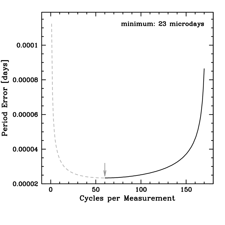
Figure 1: PEC algorithm analysis of a 90-day time series of a strictly periodic variable with a period $P$$=$$0.5274$ days and a timing uncertainty (half-bin width) of $\sigma$$=$$0.0104$ days (15 min). The arrow points to the minimum of the curve which is 23 microdays at 60 cycles per measurement.

Figure 1 shows the PEC algorithm analysis of a 90-day time series observation of a strictly periodic variable with a period $P$$=$$0.5274$ days and a timing uncertainty (half-bin width) of $\sigma\!=\!0.0104$ days (15 min). The solid curve shows the progress of the PEC algorithm as it starts with one 170-cycle measurement and progresses to the left until it includes 111 60-cycle measurements where upon it finds the optimal (minimum) period error estimate of 23 microdays which is based on 6216 individual measurements each of which has a minimum of 60-cycles per measurement. The dashed curve shows how the solution becomes progressively worse if one chooses to ignore the stopping condition of the minimum function in Equation (23) by including more and more lower-quality measurements with fewer than 60 cycles per measurement. In this example, the stopping point of 60-cycles measurements is independent of the value of the timing uncertainty, $\sigma$, because $\sigma_{\rm{PEC}}$ is linearly proportional to the value of the timing uncertainty (see Equations (23) and (24)); reducing $\sigma$ by a factor of 100 from 15 min to 9 s (0.000104 days) gives a period error estimate that is 100 times smaller than before: 0.23 microdays.

The use of the minimum function in Equation (23) as a stopping condition is required in order to obtain the optimal (minimum) value for the period error estimate. Note that the value of the summation elements within the square brackets shown in the third column of Table 1 successively decrease. Once the value of the summation elements start increasing, the value of the summation will be greater than the minimum value. Consider the case where we only include one single $M$-cycle measurement of an observation that is $M$ cycles long ($i=1$):

$$f(1;\sigma,M)=\frac{1}{1}\sum_{j=1}^{1}\frac{2\sigma^{2}}{j\left(M-(j-1)\right)^{2}}=\frac{2\sigma^{2}}{M^{2}}\,.$$ (25)

This gives period error estimates of $\sigma/\sqrt{2}$ and $\sigma/\sqrt{8}$, respectively, for a 2-cycle and a 4-cycle observation, as previously shown in Equations (6) and (13) . Now consider the case where all possible measurements are made ($i=M$, where $M>1$):

$$f(M;\sigma,M)=\frac{1}{M}\sum_{j=1}^{M}\frac{2\sigma^{2}}{j\left(M-(j-1)\right)^{2}}=\frac{1}{M}\left[\frac{2\sigma^{2}}{M^{2}}+\ldots+\frac{2\sigma^{2}}{M}\right]\,.$$ (26)

This gives a period error estimate of $\sim\!0.8660\,\sigma$ for a 2-cycle observation, which is larger than the optimal period estimate of $\sigma_{\rm{PEC}}\approx 0.7071\,\sigma$ (see Table 1 and Equation (6)). This gives a period error estimate of $\sim\!0.4751\,\sigma$ for a 4-cycle observation, which is larger than the optimal period estimate of $\sigma_{\rm{PEC}}\approx 0.3436\,\sigma$ (see Table 1 and Equation (17)). The fact that the last summation element ($2\sigma^{2}\!/M$) in Equation (26) is larger than the first summation element ($2\sigma^{2}/M^{2}$) indicates that one should never include (except in the simplest case of $M$=1) measurements of 1-cycle observations when determining period error estimates because doing so will produce a worse period error estimate than if one just measured a single $M$-cycle observation. That is why no 1-cycle observations are included in Table 1 except when $M$=1 . The stopping condition of the minimum function in Equation (23) ensures that only measurements which improve the period error estimate are used in the computation of $\sigma_{\rm{PEC}}$.

3 PERIOD ERROR ESTIMATES FOR THE KEBC

We have shown above how period error estimates of eclipsing binaries can be determined with many days of idealized uninterrupted (space based) observations. Estimating the period errors of eclipsing binary systems based on many days of real Kepler Mission long-cadence observations is slightly more complicated.

The above examples assume high signal-to-noise observations in that the expectation is that the integrated peak flux is observed in the cadence when the peak flux actually occurred. This assumption should be appropriate for most of the Kepler light curves studied in this article. However, with low S/N observations photon noise can cause “bin-hopping” where the integrated peak flux is found in neighboring cadences (measurements). This phenomenon with low S/N observations can conservatively be accounted for by tripling the timing uncertainty of high S/N observations (0.5-bin width to 1.5-bin width) which implies that the true peak may actually occur one cadence before or after the cadence with the maximum (peak) flux value. Period errors scale with the timing uncertainty and so the downside of this “fix” is that the resultant period error will be three times worse than in the high S/N case.

The total integration time for a normal Kepler long cadence observation is about 1765.5 s ($\,=\!29.4$ min) (see Figure 20 of Christiansen et al., 2012) which rounds up to the commonly used approximation of 30 min. An integration time of 30 min is an excellent approximation of the 29.4 min (a 2% error) integration time of real Kepler long cadence observations.

The quoted times for any Kepler cadence observation are believed to be accurate to within $\pm$50 ms (Koch et al., 2010; Christiansen et al., 2012; Fraquelli & Thompson, 2012), but this has not yet been tested with astrophysical data (Christiansen et al., 2012). The Kepler Data Characteristics Handbook (Christiansen et al., 2012) warns users who require temporal accuracy better than one minute that they should read Section 6 (Time and Time Stamps) carefully. The 50 ms timing accuracy for Kepler was a requirement that was levied on Ball Aerospace (the Kepler Mission prime contractor) in the top level Kepler Science Requirement Document and the Mission Requirement Document, both written in 2002, but are not generally available (Douglas Caldwell, private communication 2013). The 50 ms timing uncertainty was reported in Table 1 of Koch’s Kepler Mission overview ApJ Letter (Koch et al., 2010). Since the actual timing accuracy of the Kepler spacecraft has yet to be tested with astrophysical data, researchers should use the $\pm$50 ms timing accuracy requirement as a systematic error rather than a random error which can be beaten down with many measurements. Until the timing accuracy of the Kepler spacecraft is proven to be better than 50 ms, no more than six decimal places should be reported for any period measured in days from Kepler observations of periodic variables in the Kepler Field.

The timing uncertainty of a light curve peak found in a Kepler long cadence observation of a periodic variable is not the $\pm$50 ms timing uncertainty of the Kepler clock. Since Kepler long cadence observations are long integrations — all that one really knows for sure is the peak flux occurred sometime during the $\sim$1765.5 s of exposure time. Using a one-sixth bin width as a timing uncertainty ($1\,\sigma$) will ensure that the peak actually did occur within the long cadence observation with a $\sim\,$99.7% ($\pm$3$\sigma$) probability. Unfortunately, such a timing uncertainty gives too high a probability of the peak occurred near the middle of the observation rather than near the beginning or end of the observation. Using a half-bin width as a timing uncertainty ($1\,\sigma$) is a more realistic approximation of the timing uncertainty — even though the use of that value implies that the peak occurs within the observation only $\sim\,$68.3% ($\pm$1$\sigma$) of the time rather than the expected 100% probability (assuming high signal-to-noise observations). It is prudent to be conservative rather than to add a hidden bias to a statistical analysis.

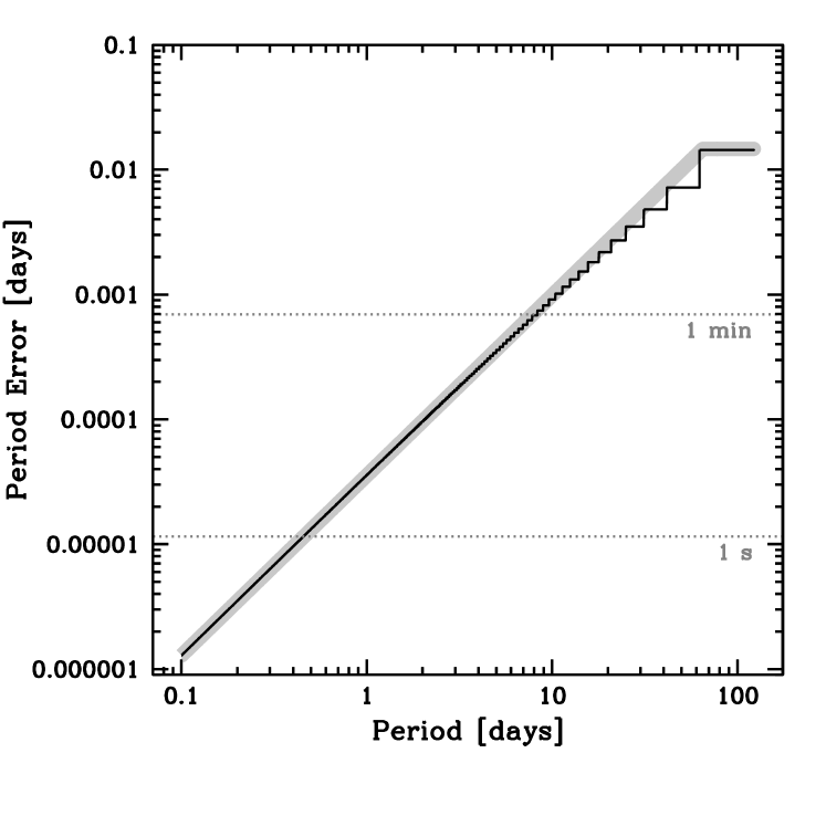
Figure 2: The jagged curve shows the results of the PEC algorithm analysis for the period errors of the Kepler Eclipsing Binary Catalog. The gray curve shows the analytical model of the PEC results.

The predicted period errors of the Kepler Eclipsing Binary Catalog are shown as the jagged curve of Figure 2. The curve is the PEC algorithm analysis of an uninterrupted 125-day time series observations of strictly periodic variables with periods ranging from 0.1 days to 125 days and a timing uncertainty (half-bin width) of $\sigma\!=\!0.0102$ days (14.7 min). The curve is jagged for longer periods because there are only so many integer number of long cycles that can be fit into a 125-day time series. The extreme example of this is that it is only possible to get one single period measurement of a periodic variable with a period between 62.5 and 125 days during a single 125-day time series and the predicted period errors are all the same: $0.0144$ $(=\sqrt{2}\,\sigma)$ days (20.8 min).

The period errors estimated by the PEC algorithm are optimistic compared to real Kepler observations. While the vast majority of Kepler observations are excellent, some fraction of the observations are problematic. The Kepler pipeline has matured sufficiently since the start of the Kepler Mission such that users of the Kepler Data Archive can now confidently reject most “bad” data by simply not using observations with SAP_QUALITY values greater than zero.

The PEC algorithm assumes continuous observations — which may or may not describe any given Kepler observation. Long observations of a target will have bad observations (SAP_QUALITY $>0$) or may contain a gap as large as $\sim\,$24 hours when no observations were obtained because the Kepler spacecraft moved off the Kepler Field in order to position itself to download all the observations obtained during the previous month.

Missing data is missing information. If many entire cycles are missing from the time series (e.g., gaps due to data download sessions), then period errors estimated from such patchy data may well be greater than they would have been with 100% coverage. However, if the data loss occurs cleanly between the eclipse and transit of a long-period detached eclipsing binary, then the period error estimate may be as good as what could have been determined without any data loss.

A simple model that approximates the upper envelope of the jagged curve of the PEC algorithm predicted period errors can be easily developed. The PEC algorithm predicts period errors of 1.2861 and 35.622 microdays for two variables with periods of $0.1$ and $1$ days, respectively. After converting these predicted errors into common (base 10) logarithm values and doing some simple arithmetic, the following simple model estimates the period errors for the Kepler Eclipsing Binary Catalog:

$$\sigma_{\rm{KEBC}}\approx\left\{\begin{array}[]{l}10^{-5.8908+1.4425\,\left(\log(P_{\rm{KEPC}})+1\right)}{\rm{~{}days}}\,,\\ {\rm{\hskip 20.0ptif~{}}}P_{\rm{KEBC}}<62.5{\rm{~{}days}}\,;\\ 0.0144{\rm{~{}days\,,}}{}\\ {\rm{\hskip 20.0ptif~{}}}P_{\rm{KEBC}}\geq 62.5{\rm{~{}days;}}\end{array}\right.$$ (27)

where $P_{\rm{KEBC}}$ is the period of the variable in the KEPC in units of days. This model is shown as the thick gray curve in Figure 2. The PEC algorithm predicts a period error of 180 microdays for a strictly periodic variable with a period $P\!=\!3.17$ days; Equation (27) predicts a period error of 190 microdays (an error of 5.6% greater than the PEC algorithm estimate). The PEC algorithm predicts a period error of 910 microdays for a period $P\!=\!10$ days; the model predicts a period error of 990 microdays (an error of 8.8%). The PEC algorithm predicts a period error of 7.2 millidays for a period $P\!=\!41.69$ days; the model predicts a period error of 7.7 millidays (an error of 6.9%).

So far, we have only considered theoretical predictions for period errors. How well do these predicted period error estimates compare to real period error measurements based on Kepler long cadence observations of two semidetached and five detached eclipsing binaries and an RR Lyrae variable star?

The NASA Exoplanet Archive Periodogram Service is a U.S. Virtual Astronomical Observatory (VAO) web service (VAO, 2011, 2012) that searches for periodic signals in exoplanet observations from the NASA Kepler and the ESA CoRoT astrophysical missions or in user-provided observations of time and flux of variable astronomical objects. The Periodogram Service returns periodograms of time series data. Users can download the derived periodograms as well as the phased light curves for the five most significant periods determined from the data. Unfortunately, no period error estimates are provided for any significant periods.

At the beginning of every Kepler quarter since Q2, the Kepler spacecraft rotates 90$\arcdeg$ in order to optimize the orientation of the solar panels on spacecraft with respect to the Sun. As a consequence of this roll, when the spacecraft resumes its normal operations, light from a given target now falls on a different CCD than was used in the previous quarter. Individual Kepler observations are not flux calibrated in an absolute sense and so there can be considerable jumps (up and down) in the measured flux of a given target from quarter to quarter — even if there is no evidence for variability in the target and the same aperture is used. If one wishes to analyze multiple quarters of Kepler observations simultaneously, it is necessary to “normalize” the data from different quarters to be approximately on the same flux scale. For example, for detached eclipsing binaries with long periods, the measured flux between eclipses should be the same — from quarter to quarter. If one plots the light curve of a given target (e.g., PDCSAP_FLUX vs. TIME) for multiple Kepler quarters, one sees that the maximum and minimum flux values can vary a lot between quarters. The normalization process across multi-quarter observations can be quite complicated (e.g., see §4.2 (Data Detrending) of Slawson et al. (2011)) and is beyond the scope of this article. The Periodogram Service has recently implemented an option to normalize Kepler light curves for all public data for a given Kepler target. The Periodogram Service generally does a good job of normalizing flux values across many Kepler quarters. While the current normalization algorithm is not perfect, it is a good step in the right direction.

The Periodogram Service gives the user a choice of three algorithms for computing periodograms from light curve data: (1) Lomb-Scargle (Scargle, 1982), (2) “BLS” (Box-fitting Least Squares) (Kovács et al., 2002), and (3) Plavchan (Plavchan et al., 2008). The Lomb-Scargle algorithm is the default method used by the Periodogram Service. A description of the implementation details of these three algorithms may be found on the Algorithm Documentation webpage of the Periodogram Service.

While the Periodogram Service currently does not directly provide period error estimates for the periods it finds as peaks in the power of computed periodograms, a user of the Periodogram Service can measure the period error of a given period by using the method described below. A major drawback of this method is that it is both labor intensive for the user and computationally intensive for the 128-core computer cluster used by the Periodogram Service (seconds to minutes per eclipsing binary system, depending on the current user load on the cluster).

Over a narrow range of periods near the best period estimate, periodograms of eclipsing binaries are typically bell-shaped (non-Gaussian) curves. A good estimate of the uncertainty of a period measurement is the Half-Width-at-Half-Maximum (HWHM) of the periodogram peak.

The peak of the periodogram (maximum power), produced by the Plavchan algorithm analyzing normalized Kepler observations from quarters Q0 through Q2, of the detached eclipsing binary KID 3120320 occurs at 10.2656 days and the Full-Width-at-Half-Maximum (FWHM) of the periodogram peak is 5.6 millidays wide (see Figure 3). This periodogram was computed over a much narrower period range (9.75–10.75 days) and at a much higher resolution (430$\times$) in frequency-space and with a much higher resolution phase-smoothing box size (30$\times$) than is normally provided by default by the Periodogram Service using the Plavchan method: fixed df step size of 0.000001 and a phase-smoothing box size of 0.002 . All of these modifications to the default parameters must be done by hand by the user because, as of now, such changes can not be done remotely using a computer script.

The uncertainty of the period estimate is approximately the HWHM: 2.8 millidays. The period estimate of KID 3120320 is thus $P\!=\!10.2656(28)$ days, which agrees exactly with the Kepler Eclipsing Binary Catalog estimate of 10.265600 days — but the last 2 digits of the KEBC period are probably not significant.

The Plavchan algorithm was found to produce more precise periods and period error measurements of Kepler observations of eclipsing binaries than the Lomb-Scargle and BLS algorithms. With the same data for KID 3120320, the Lomb-Scargle algorithm gave a period of 10.20(31) days while the BLS algorithm gave a period of 10.24(11) days. In this case, the Plavchan algorithm produced two more significant digits of precision for the period measurement as compared with the Lomb-Scargle and the BLS algorithms.

The top two sections of Table 2 gives the period and period error measurements of 7 eclipsing binaries in the Kepler Eclipsing Binary Catalog with periods ranging from $\sim\,$0.5 to $\sim\,$50 days. The first column gives the Kepler quarters that were used in the analysis; Kepler quarters Q0 through Q2 were normally used (as was done with the KEBC) but in the case of KID 9540450 there were no Q0 observations. The second column gives the unique Kepler Identification number (KID) for each target. The third column gives the type of eclipsing binary system of the target; the two shortest period systems are semi-detached eclipsing binaries and the rest are detached eclipsing binaries. The fourth column gives the brightness the target in Kepler magnitudes (KEPMAG) as given in the Kepler Input Catalog (KIC) (Brown et al., 2011). The fifth column gives the period of the target as given in the KEBC. The sixth column gives the measured period and period error as determined using the Periodogram Service. The last column gives the period error estimate of the PEC algorithm (Equation (23)) for a uninterrupted 125-day time series and a timing uncertainty (half-bin width) of 0.0102 days $\left[=\!\left(29.4{\rm{~{}min}}\right)/2\right]$.

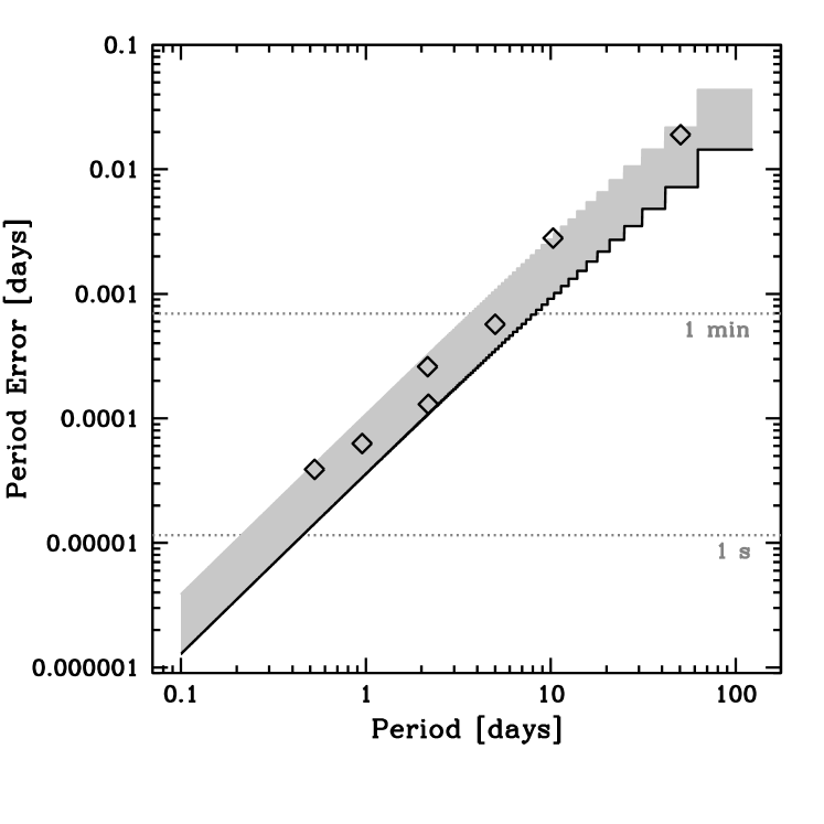
Figure 4: The jagged curve shows the results of the PEC algorithm analysis for the period errors of the Kepler Eclipsing Binary Catalog (same as Figure 2). The diamonds show the measured period errors of the seven eclipsing binaries given in Table 2. The gray region shows where accurate and precise period error measurements are expected to be found.

The measured period errors for the top section of Table 2 for the eclipsing binary systems KID 11560447, 10858720, 9873869, 3120320, and 9172506 are, respectively, 39, 63, 570 microdays, and 2.8, 19 millidays (shown as diamonds in Figure 4). These measured period errors are larger than the PEC algorithm estimate by factors of 2.8, 1.9, 1.7, 3.1, and 2.6, respectively.

The middle section of Table 2 investigates how the measured period error changes as a function of brightness of two eclipsing binaries with nearly identical periods ($P\!\approx\!2.16$ days). The detached eclipsing binary systems KID 9641031 and 9540450 have Kepler magnitudes of 9.177 and 14.146 mag with measured period errors of 0.13 and 0.26 millidays respectively. Bright eclipsing binary systems have smaller period errors than faint systems with the same period.

The gray region in Figure 4 shows where accurate and precise period error measurements of systems in the Kepler Eclipsing Binary Catalog are expected to be found. The bottom limit of the gray region is the jagged curve shown in Figure 2; high S/N observations are expected to be found near the bottom limit. The top limit of the gray region is 3 times the jagged curve shown in Figure 2; low S/N observations are expected to be found near the top limit. Note that the measured period errors of the seven eclipsing binaries in Table 2 lie within or very near the gray region in Figure 4. As expected, the bright eclipsing binary KID 9641031 ($P$=2.17816(13) days, 9.177 mag) lies near the bottom limit of the gray region while the faint binary KID 9540450 ($P$=2.15472(26) days, 14.146 mag) lies just slightly above the top limit of the gray region ($3.1\sigma_{\rm{PEC}}$ instead of $3\sigma_{\rm{PEC}}$).

While very bright eclipsing binary systems in the Kepler Eclipsing Binary Catalog can nearly achieve the period errors predicted by the PEC algorithm (see Figure 4), for most eclipsing binary systems in the KEBC, the period errors predicted by the PEC algorithm are likely to be the lower limit of the true period errors. In other words, most periods in the KEBC are likely to have uncertainties that are larger than the period error estimated using the PEC algorithm. Nevertheless, the PEC algorithm (Equation (23)) or its approximation for the KEBC (Equation (27)) can provide useful limits to the true precision of periods in the KEBC.

4 DISCUSSION

The information content of the phased light curve of long-period detached eclipsing binaries is low — only observations obtained during a transit (primary eclipse) or secondary eclipse offer useful information about the period.

The PEC algorithm predicts period errors based only on a single feature (the peak/minimum value) of each cycle of a strictly periodic variable. If the phased light curve of a strictly periodic variable is morphologically complicated, then the period error estimated by the PEC algorithm can be reduced by a factor of $\sqrt{n}$ if $n$ unique features can be robustly identified in each cycle of observation. For example, if it is possibly to unambiguously identify both the maximum and minimum of a light curve during each cycle of observation, then the PEC algorithm period estimate can be reduced by a factor of $\sqrt{2}$.

Theoretically, the more unique features one can measure, the better the improvement will be — but one quickly encounters a situation of diminishing returns. Suppose we analyze Kepler long cadence observations of a RR Lryae variable with a period of 0.5 days. Phased light curves of RR Lyrae are much richer morphologically than phased light curves of eclipsing binaries. There will be 24 Kepler long cadence observations per cycle (period). An improvement of $\sqrt{24}$ over the PEC algorithm period error estimate would be the best possible case. But that would require a unique “feature” to be present in every single Kepler long cadence observation.

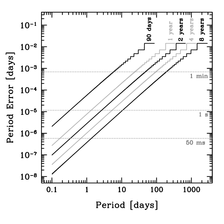
Figure 5: Period errors determined with the PEC algorithm for Kepler long cadence observations with durations of 90 days, 1 year, 2 years, 4 years, and 8 years.

The last section of Table 2 investigates how the measured period error of FN Lyrae (KID 6936115), a non-Blashko ab-type RR Lyrae (Nemec et al., 2011), compares to the PEC algorithm period error estimates. Using the Periodogram Service to analyze Kepler quarter Q2 observations, we determined that the period of FN Lyr is 0.5273989 days with an uncertainty of 4.4 microdays. The PEC algorithm gives a period error estimate of 23 microdays for an uninterrupted 88.9-day (DAWG, 2012a) time series and a timing uncertainty (half-bin width) of 0.0102 days. The measured period error is a factor of 5.2 times better than the PEC algorithm estimate and is slightly better than the estimated “best possible case”: 4.6 microdays ($\approx$23 microdays$/\sqrt{24}$) assuming that all cadences have a unique feature. Using the Periodogram Service to analyze seven normalized Kepler quarters of observations (Q2 through Q8), the period of FN Lyr was determined to be 0.5273989 days with an uncertainty of 1.4 microdays. Although the period estimate is the same as before, the uncertainty of the measurement has been reduced by a factor of 3.1. The PEC algorithm gives a period error estimate of 1.4 microdays for an uninterrupted 608.9-day (DAWG, 2012a, b) time series and a timing uncertainty (half-bin width) of 0.0102 days. Note that the measured period error using 7 Kepler quarters (Q2–Q8) agrees exactly with the PEC algorithm estimate. Figure 5 may prove useful for planning future Kepler Mission observations of eclipsing binaries and other periodic variables in the Kepler Field.

The PEC algorithm was devised to provide a reasonable estimate of the periods published in the Kepler Eclipsing Binary Catalog. Figure 4 shows that this goal has been accomplished. The PEC algorithm was used to estimate the period errors of seven eclipsing binaries from the KEBC (see Table 2). All seven error estimates were found in or near the gray region of Figure 4 which has lower and upper limits set by the PEC algorithm assuming, respectively, high and low S/N measurements of the Kepler light curves. While not perfect, the PEC algorithm is certainly a lot better than what we have now with regards to KEBC period error estimates — nothing at all.

The big advantage of the PEC algorithm is that it is a quick-look method for the determination of period error estimates for long time series observations of eclipsing binaries. It is fast and does not require any detailed analysis of actual light curve data; all that is required are 3 numbers in units of days: (1) the estimated period of the strictly periodic variable, (2) the timing uncertainty for a single measurement (0.0102 days for a Kepler long cadence observation), and (3) the total length of the continuous observation. The curators of the NASA Exoplanet Archive Periodogram Service are encouraged to enhance the Periodogram Service by adding PEC algorithm period error estimates when it reports likely periods based on periodogram analysis of Kepler light curves of periodic variables.

In our description of the PEC algorithm we have referred to strictly periodic eclipsing binary systems. Some eclipsing binaries, however, undergo period changes. Sometimes those changes are due to the gravitational effects of a third body (e.g., Hoffman et al., 2006). Sometimes those changes can be due to mass transfers in compact eclipsing binary systems (e.g., Zhu et al., 2012). Starspots as well as photometric noise can also cause subtle timing changes of light curve minima (Kalimeris et al., 2002). Period changes are usually detected using $O-C$ diagrams where the difference between observed time, $O$, of a light curve extremum (transit or eclipse) and the computed (predicted) time, $C$, is plotted using an ephemeris model. Eclipsing binary systems with significant $O-C$ differences are, by definition, not strictly periodic and thus the true period error estimate for these systems will be larger than that predicted by the PEC algorithm. Finding significant $O-C$ differences generally requires a detailed inspection of the actual light curve. Now if a non-strictly periodic eclipsing binary system were to be continuously observed by Kepler over the course of many years, it might be possible to detect such systems by comparing the differences of orbital periods derived, from say yearly baselines, to the PEC period error estimate for one year of Kepler observations. If the $O-C$ differences only become significant over a period of many years or decades, then the detection of such non-strictly periodic systems by Kepler using the PEC period error estimate might not be possible due to its currently envisioned maximum lifetime of 7.5 years for the Kepler Mission.

The neural networks currently being used by the EBAI method could be improved to include the computation of confidence intervals for the eclipsing binary parameters determined by its neural networks. That might require a complete rewrite of the current neural network software framework used by the EBAI method, which would probably be a time-consuming expensive exercise. Although the end result may well be worth the effort, especially in the era of a fully operational LSST (Large Synoptic Survey Telescope) project, acquiring the necessary resources to make such significant changes might be challenging. Alternatively, such an effort could possibly be cast as an astrophysics Ph.D. dissertation project with a major focus on applied information systems research.

Nemec et al. (2011) report that the period of FN Lyr is 0.527398471(4) days based on Kepler Q0 through Q5 observations. That period error estimate is just 4 nanodays — which is a factor of 145 smaller than the 50 ms (579 nanodays) timing accuracy of the Kepler spacecraft. “Typically, the periods derived using the Q0-Q5 LC data alone are accurate to 1–$2\times 10^{-7}$ days” Nemec et al. (2011) . Assuming a conservative 200 nanoday period error estimate, that is still a factor of 2.90 times smaller than 50 ms. The period error estimates of Nemec et al. (2011) are the average of period estimates obtained by the three methods available with the software package Period04 (Lenz & Breger, 2004, 2005). The averaging of results from three different methods is not a proper error analysis — all three methods might be driven by the data to produce period estimates with more digits of precision than are significant. The PEC algorithm predicts a period error of 2.6 microdays (220 ms) for an uninterrupted 406-day (DAWG, 2012a, b) time series and a timing uncertainty (half-bin width) of 0.0102 days. The lower limit for the PEC algorithm period error estimate is 531 nanodays ($\approx 2.6\,{\rm{microdays}}/\sqrt{24}$) which is just below the 50 ms timing uncertainty for Kepler.

In a search for third star companions in 41 eclipsing binaries observed by the Kepler Mission, Gies et al. (2012) give the properties of these systems in their Table 1. The periods and period error estimates were based on all the long cadence Kepler light curve observations through Kepler quarter Q9. Only 2 of the 41 systems had period error estimates greater than the 50 ms timing uncertainty for Kepler: the best period error estimate is 2 nanodays and the worst is 20 microdays; the median is 30 nanodays. A period estimate of 1.404678238 days with an uncertainty of 8 nanodays was given for the primary star of the eclipsing binary KID 2305272. The PEC algorithm gives a period error estimate of 4.0 microdays for a uninterrupted 803-day (DAWG, 2011, 2012a, 2012b) time series and a timing uncertainty (half-bin width) of 0.0102 days. In order to achieve a precision of 8 nanodays with the PEC algorithm, one needs a timing uncertainty of about 20 microdays (1.7 s) on every Kepler observation. That timing accuracy is at the very bottom of the range of internal timing measurement errors (1 to 318 s) reported by Gies et al. (2012). With 67.2 Kepler long cadence observations during a single cycle (period) of KID 2305272, the lower limit for the PEC algorithm period error estimate is 0.5 microdays ($\approx 4.0\,{\rm{microdays}}/\sqrt{67}$) which is below the 50 ms limit. The timings used by Gies et al. (2012) were based on model fitting of parabolas to the lowest 20% to the “eclipse template data” in order to find the actual phase of the eclipse minimum. It is not clear how the eclipse template data was mitigated to account for the long exposures times of $\sim\,$1765.5 s.

The period errors estimated by the PEC algorithm are not the best possible period errors that can be obtained for eclipsing binary systems. If a lot more effort is expended, then better period error estimates can usually be determined. The best period error estimates for the orbital periods of eclipsing binary systems are generally determined using least-squares model-fitting techniques on precision observations of photometry and radial velocities. By comparing relative fluxes and radial velocities to physically detailed models of an eclipsing binary system, all photometric and radial velocity information about the system can be optimized simultaneously. For example, Van Hamme & Wilson’s (2007) study of the bright ($7.71\!\leq\!V\!\leq\!8.48$ mag; Kukarkin et al. 1971) triple-system (Hilditch et al. 1986) Algol-type eclipsing binary DM Persei yielded a period error estimate of 180 nanodays by using intermittent observations over decades of ground-based photometry and radial velocity measurements: $P_{0}=2.72774109(18)$ days. Mikulášek et al. (2012) have presented a promising method for the period analysis of eclipsing binaries which does not use $O-C$ diagrams. This method was used by Zhu et al. (2012) to determine the period of the relatively bright ($11.0\!\leq\!V\!\leq\!11.6$ mag; Kukarkin et al. 1971) close eclipsing binary BS Vulpecula with a period error estimate of 20 nanodays: $P_{0}=0.47597002(3)$ days. Whether such precision is truly plausible remains to be seen when this new method is applied in the future to other eclipsing binary systems.

Table 1: Square of Period Error Estimates for 1 to 7 Cycles

M	Expanded	Reduced
1	$\displaystyle({\sigma^{2}_{2}}+{\sigma^{2}_{1}})$	$\displaystyle 2\sigma^{2}$
2	$\displaystyle\frac{1}{2^{2}}({\sigma^{2}_{3}}+{\sigma^{2}_{1}})$	$\displaystyle\frac{\sigma^{2}}{2}$
3	$\displaystyle\frac{1}{3^{2}}({\sigma^{2}_{4}}+{\sigma^{2}_{1}})$	$\displaystyle\frac{2\sigma^{2}}{9}$
4	$\displaystyle\frac{1}{2}\bigg{[}\,\frac{1}{4^{2}}({\sigma^{2}_{5}}+{\sigma^{2}_{1}})$	$\displaystyle\frac{\sigma^{2}}{2}\bigg{[}\frac{1}{8}$
	$\displaystyle~{}~{}+\frac{1}{2^{2}\times 3^{2}}\Big{(}({\sigma^{2}_{5}}+{\sigma^{2}_{2}})+({\sigma^{2}_{4}}+{\sigma^{2}_{1}})\Big{)}\bigg{]}$	$\displaystyle~{}~{}~{}~{}+\frac{1}{9}\bigg{]}$
5	$\displaystyle\frac{1}{2}\bigg{[}\,\frac{1}{5^{2}}({\sigma^{2}_{6}}+{\sigma^{2}_{1}})$	$\displaystyle\frac{\sigma^{2}}{2}\bigg{[}\frac{2}{25}$
	$\displaystyle~{}~{}+\frac{1}{2^{2}\times 4^{2}}\Big{(}({\sigma^{2}_{6}}+{\sigma^{2}_{2}})+({\sigma^{2}_{5}}+{\sigma^{2}_{1}})\Big{)}\bigg{]}$	$\displaystyle~{}~{}~{}~{}+\frac{1}{16}\bigg{]}$
6	$\displaystyle\frac{1}{3}\bigg{[}\,\frac{1}{6^{2}}({\sigma^{2}_{7}}+{\sigma^{2}_{1}})$	$\displaystyle\frac{\sigma^{2}}{3}\bigg{[}\frac{1}{18}$
	$\displaystyle~{}~{}+\frac{1}{2^{2}\times 5^{2}}\Big{(}({\sigma^{2}_{7}}+{\sigma^{2}_{2}})+({\sigma^{2}_{6}}+{\sigma^{2}_{1}})\Big{)}$	$\displaystyle~{}~{}~{}~{}+\frac{1}{25}$
	$\displaystyle~{}~{}+\frac{1}{3^{2}\times 4^{2}}\Big{(}({\sigma^{2}_{7}}+{\sigma^{2}_{3}})+({\sigma^{2}_{6}}+{\sigma^{2}_{2}})+({\sigma^{2}_{5}}+{\sigma^{2}_{1}})\Big{)}\bigg{]}$	$\displaystyle~{}~{}~{}~{}+\frac{1}{24}\bigg{]}$
7	$\displaystyle\frac{1}{4}\bigg{[}\,\frac{1}{7^{2}}({\sigma^{2}_{8}}+{\sigma^{2}_{1}})$	$\displaystyle\frac{\sigma^{2}}{4}\bigg{[}\frac{2}{49}$
	$\displaystyle~{}~{}+\frac{1}{2^{2}\times 6^{2}}\Big{(}({\sigma^{2}_{8}}+{\sigma^{2}_{2}})+({\sigma^{2}_{7}}+{\sigma^{2}_{1}})\Big{)}$	$\displaystyle~{}~{}~{}~{}+\frac{1}{36}$
	$\displaystyle~{}~{}+\frac{1}{3^{2}\times 5^{2}}\Big{(}({\sigma^{2}_{8}}+{\sigma^{2}_{3}})+({\sigma^{2}_{7}}+{\sigma^{2}_{2}})+({\sigma^{2}_{6}}+{\sigma^{2}_{1}})\Big{)}$	$\displaystyle~{}~{}~{}~{}+\frac{2}{75}$
	$\displaystyle~{}~{}+\frac{1}{4^{2}\times 4^{2}}\Big{(}({\sigma^{2}_{8}}+{\sigma^{2}_{4}})+({\sigma^{2}_{7}}+{\sigma^{2}_{3}})+({\sigma^{2}_{6}}+{\sigma^{2}_{2}})+({\sigma^{2}_{5}}+{\sigma^{2}_{1}})\Big{)}\bigg{]}$	$\displaystyle~{}~{}~{}~{}+\frac{1}{32}\bigg{]}$

Table 2: Period Errors of Variables in the Kepler Field

Kepler	KID	Type	KEPMAG	$P_{\rm{KEBC}}$	$P$	$\sigma_{\rm{PEC}}$
Quarters			(mag)	(days)	(days)	(days)
Q0–Q2	11560447	SD	10.834	0.527680	0.527678(39)	0.000014
Q0–Q2	10858720	SD	10.971	0.952386	0.952372(63)	0.000033
Q0–Q2	9873869	D	13.038	4.994774	4.99477(57)	0.00034
Q0–Q2	3120320	D	10.885	10.265600	10.2656(28)	0.00091
Q0–Q2	9172506	D	12.009	50.440245	50.442(19)	0.0072
Q0–Q2	9641031	D	9.177	2.178152	2.17816(13)	0.00011
Q1–Q2	9540450	D	14.146	2.154687	2.15472(26)	0.00011
Q2	6936115	RR Lyr	12.876	$\cdots$	0.5273989(44)	0.000023
Q2–Q8	6936115	RR Lyr	12.876	$\cdots$	0.5273989(14)	0.0000014

Figure 3: Periodogram of the Plavchan algorithm analysis of normalized Kepler Q0, Q1, and Q2 observations of the detached eclipsing binary KID 3120320. The dotted line is the Full-Width-at-Half-Maximum (FWHM) which is 5.6 millidays wide. The measured period for KID 3120320 is 10.2656(28) days.

References

- Bevington (1969) Bevington, P. R. 1969, Data reduction and error analysis for the physical sciences (New York: McGraw-Hill Book Co.)
- Borucki et al. (2011) Borucki, W. J., Koch, D. G., & Basri, G., et al. 2011, ApJ, 728, 117
- Brown et al. (2011) Brown, T. M., Latham, D. W., Everett, M. E., & Esquerdo, G. A. 2011, AJ, 142, 112
- Christiansen et al. (2012) Christiansen, J. L., Van Cleve, J. E., & Jenkins, J. M., et al. 2012, Kepler Data Characteristics Handbook (March, 2012), KSCI-19040-003
- DAWG (2011) DAWG. 2011, Kepler Data Release Notes 12: Q9, Data Analysis Working Group (DAWG), KSCI-19052-001
- DAWG (2012a) —. 2012a, Kepler Data Release Notes 14: Q0–Q4, Data Analysis Working Group (DAWG), KSCI-19054-001
- DAWG (2012b) —. 2012b, Kepler Data Release Notes 16: Q5–Q8, Data Analysis Working Group (DAWG), KSCI-19056-001
- DAWG (2013) —. 2013, Kepler Data Release Notes 19: Q14, Data Analysis Working Group (DAWG), KSCI-19059-001
- Fraquelli & Thompson (2012) Fraquelli, D. & Thompson, S. E. 2012, Kepler Archive Manual – Revision 4, KDMC-10008-004
- Gies et al. (2012) Gies, D. R., Williams, S. J., & Matson, R. A., et al. 2012, AJ, 143, 137
- Hilditch et al. (1986) Hilditch, R. W., Skillen, I., Carr, D. M., & Aikman, G. C. L. 1986, MNRAS, 222, 167
- Hoffman et al. (2006) Hoffman, D. I., Harrison, T. E., & McNamara, B. J., et al. 2006, AJ, 132, 2260
- Kalimeris et al. (2002) Kalimeris, A., Rovithis-Livaniou, H., & Rovithis, P. 2002, A&A, 387, 969
- Koch et al. (2010) Koch, D. G., Borucki, W. J., & Basri, G., et al. 2010, ApJ, 713, L79
- Kovács et al. (2002) Kovács, G., Zucker, S., & Mazeh, T. 2002, A&A, 391, 369
- Kukarkin et al. (1971) Kukarkin, B. V., Kholopov, P. N., & Pskovskij, Y. P., et al. 1971, General catalogue of variable stars. Volume III.
- Lenz & Breger (2004) Lenz, P. & Breger, M. 2004, The A-Star Puzzle, 224, 786
- Lenz & Breger (2005) —. 2005, Communications in Asteroseismology, 146, 53
- Mighell (2013) Mighell, K. J. 2013, PEC, Astrophysics Source Code Library, record: ascl:1304.001
- Mikulášek et al. (2012) Mikulášek, Z., Zejda, M., & Janík, J. 2012, IAU Symposium, 282, 391
- Nemec et al. (2011) Nemec, J. M., Smolec, R., & Benkő, J. M., et al. 2011, MNRAS, 417, 1022
- Plavchan et al. (2008) Plavchan, P., Jura, M., Kirkpatrick, J. D., Cutri, R. M., & Gallagher, S. C. 2008, ApJS, 175, 191
- Prša et al. (2011) Prša, A., Batalha, N., & Slawson, R. W., et al. 2011, AJ, 141, 83
- Prša et al. (2008) Prša, A., Guinan, E. F., & Devinney, E. J., et al. 2008, ApJ, 687, 542
- Scargle (1982) Scargle, J. D. 1982, ApJ, 263, 835
- Slawson et al. (2011) Slawson, R. W., Prša, A., & Welsh, W. F., et al. 2011, AJ, 142, 160
- Van Hamme & Wilson (2007) Van Hamme, W. & Wilson, R. E. 2007, ApJ, 661, 1129
- VAO (2011) VAO. 2011, Virtual Astronomical Observatory Annual Report For the Period: 15 May 2010 Through 30 April 2011
- VAO (2012) —. 2012, Virtual Astronomical Observatory Annual Report For the Period: 1 May 2011 Through 30 April 2012
- Zhu et al. (2012) Zhu, L.-Y., Zejda, M., & Mikulášek, Z., et al. 2012, AJ, 144, 37