Theory-based Benchmarking of the Blended Force-Based Quasicontinuum Method

Abstract.

We formulate an atomistic-to-continuum coupling method based on blending atomistic and continuum forces. Our precise choice of blending mechanism is informed by theoretical predictions. We present a range of numerical experiments studying the accuracy of the scheme, focusing in particular on its stability. These experiments confirm and extend the theoretical predictions, and demonstrate a superior accuracy of B-QCF over energy-based blending schemes.

1. Introduction

Atomistic-to-continuum coupling methods (a/c methods) have been proposed to increase the computational efficiency of atomistic computations involving the interaction between local crystal defects with long-range elastic fields [7, 22, 29, 40, 15, 30, 6, 18]; see [26] for a recent review of a/c coupling methods and their numerical analysis. Energy-based methods in this class, such as the quasicontinuum model (denoted QCE [41]), exhibit spurious interfacial forces (“ghost forces”) even under uniform strain [39, 8]. The effect of the ghost force on the error in computing the deformation and the lattice stability by the QCE approximation has been analyzed in [8, 9, 31, 10], where lattice stability refers to the positive definiteness of the Hessian matrix of the total potential energy. The development of more accurate energy-based a/c methods is an ongoing process [40, 15, 37, 38, 20, 34, 5].

An alternative approach to a/c coupling is the force-based quasicontinuum (QCF) approximation [11, 12, 7, 29, 25], but the non-conservative and indefinite equilibrium equations make the iterative solution and the determination of lattice stability more challenging [13, 12, 14]. Indeed, it is an open problem whether the (sharp-interface) QCF method is stable in dimension greater than one. Although some recent results in this direction exist [24], it is still unclear to what extent they can be extended for general atomistic domains and in the presence of defects.

Many blended a/c coupling methods have been proposed in the literature, e.g.,  [4, 2, 23, 1, 36, 16, 35, 3, 42]. In [21], we formulated a blended force-based quasicontinuum (B-QCF) method, similar to the method proposed in [25], which smoothly blends the forces of the atomistic and continuum model instead of the sharp transition in the QCF method. Under the simplifying assumption that deformation is homogeneous, we established sharp conditions under which a linearized B-QCF operator is positive definite, which effectively guarantees stability of the numerical scheme. Surprisingly, the required blending width to ensure positive definiteness of the linearized B-QCF operator is asymptotically small (however typical prefactors in the relative size of the blending region are not predicted by the theory). The one-dimensional theory developed in [21] is complete and agrees with the numerical experiments. However, the two-dimensional theory was based on a conjecture that has been proved only in a particular case (see Remark 3.1 for more details) and therefore requires numerical validation.

In the present paper, we present focused numerical experiments to validate and extend the theoretical conclusions in [21, 19]. In particular, we study (i) whether stability of the B-QCF method in 2D can be systematically improved with increasing the blending width, (ii) whether a relatively narrow blending, as suggested by the theory, is enough in practice, and (iii) whether using the quintic spline (that has the regularity assumed in the theory) has advantages over the cubic spline. In addition we provide accuracy benchmarks similar to those in [27]. Our numerical benchmarks demonstrate that the B-QCF scheme is a practical a/c coupling mechanism with performance (accuracy versus computational cost) superior to energy-based blending schemes.

1.1. Summary

In section 2, we introduce the B-QCF model for a $1$D atomistic chain. We state the asymptotically optimal condition on the blending size in Theorem 2.1 and apply a uniform expansion to the atomistic chain in subsection 2.2. The critical strain errors between the atomistic and B-QCF models with different blending size are computed in this subsection. The numerical results perfectly match the analytic prediction, that is, the errors decay polynomially in terms of the blending size.

In section 3, we establish the B-QCF model for a $2$D hexagonal lattice. We state sufficient and necessary conditions on the blending width under which the B-QCF operator is positive definite. To numerically investigate the positive-definiteness of the B-QCF operators in $2$D, we apply three different classes of deformations to the perfect lattice, which are the uniform expansion, two types of shear deformation, and a general class of homogeneous deformations. The results of $2$D uniform expansion are similar to those of the $1$D example, and they agree with the theoretical conclusions well.

The stability regions of the different models under homogeneous deformations are consistent with the analytic prediction. By using a small blending region, the $2$D B-QCF operator becomes almost as stable as the atomistic model, compared to the fact that the stability region of the force-based quasicontinuum (QCF) method, i.e., the B-QCF method without blending region, is a proper subset of the fully atomistic model [13, 12, 14]. However, the stability error under shear deformation for the B-QCF operator seems to only depend linearly on the system size, which is observed from the numerical experiments.

In section 4, we implement the B-QCF method from a practical point of view. We briefly review the accuracy results in terms of computational cost, i.e., the total number of degrees of freedom ${\rm DoF}$, and then include some numerical experiments for a di-vacancy and microcrack to demonstrate the superior accuracy of B-QCF over other a/c coupling schemes that we have investigated previously in [27].

2. The B-QCF Operator in $1$D.

2.1. Notation

We denote the scaled reference lattice by $\epsilon\mathbb{Z}:=\{\epsilon\ell:\ell\in\mathbb{Z}\}$. We apply a macroscopic strain $F>0$ to the lattice, which yields

$$\mathbf{y}_{F}:=F\epsilon\mathbb{Z}=(F\epsilon\ell)_{\ell\in\mathbb{Z}}.$$

The space $\mathcal{U}$ of $2N$-periodic zero mean displacements $\mathbf{u}=(u_{\ell})_{\ell\in\mathbb{Z}}$ from $\mathbf{y}_{F}$ is given by

$$\mathcal{U}:=\bigg{\{}\mathbf{u}:u_{\ell+2N}=u_{\ell}\text{ for }\ell\in\mathbb{Z},\text{ and }{\textstyle\sum_{\ell=-N+1}^{N}u_{\ell}}=0\bigg{\}},$$

and we thus admit deformations $\mathbf{y}$ from the space

$$\mathcal{Y}_{F}:=\{\mathbf{y}:\mathbf{y}=\mathbf{y}_{F}+\mathbf{u}\text{ for some }\mathbf{u}\in\mathcal{U}\}.$$

We set $\epsilon=1/N$ throughout so that the reference length of the computational cell remains fixed.

We define the discrete differentiation operator, $D\mathbf{u}$, on periodic displacements by

$$(D\mathbf{u})_{\ell}:=\frac{u_{\ell}-u_{\ell-1}}{\epsilon},\quad-\infty<\ell<\infty.$$

We note that $\left(D\mathbf{u}\right)_{\ell}$ is also $2N$-periodic in $\ell$ and satisfies the zero mean condition. We will often denote $\left(D\mathbf{u}\right)_{\ell}$ by $Du_{\ell}$. We then define $\left(D^{(2)}\mathbf{u}\right)_{\ell}$ and $\left(D^{(3)}\mathbf{u}\right)_{\ell}$ for $-\infty<\ell<\infty$ by

$$\left(D^{(2)}\mathbf{u}\right)_{\ell}:=\frac{Du_{\ell+1}-Du_{\ell}}{\epsilon};\quad\left(D^{(3)}\mathbf{u}\right)_{\ell}:={\frac{D^{(2)}u_{\ell}-D^{(2)}u_{\ell-1}}{\epsilon}.}$$

To make the formulas more concise, we sometimes denote $Du_{\ell}$ by $u^{\prime}_{\ell}$, $D^{(2)}u_{\ell}$ by $u^{\prime\prime}_{\ell}$, etc., when there is no confusion in the expressions.

For a displacement $\mathbf{u}\in\mathcal{U}$ and its discrete derivatives, we employ the weighted discrete $\ell_{\epsilon}^{p}$ and $\ell_{\epsilon}^{\infty}$ norms by

$$\|\mathbf{u}\|_{\ell_{\epsilon}^{p}} :=\left(\epsilon\sum_{\ell=-N+1}^{N}|u_{\ell}|^{p}\right)^{1/p}\text{for }1\leq p<\infty,\qquad\|\mathbf{u}\|_{\ell_{\epsilon}^{\infty}}:=\max\limits_{-N+1\leq\ell\leq N}|u_{\ell}|,$$

and the weighted inner product for $\ell_{\epsilon}^{2}$ is

$$\langle\mathbf{u},\mathbf{w}\rangle:=\sum\limits_{\ell=-N+1}^{N}\epsilon u_{\ell}w_{\ell}.$$

2.2. The B-QCF Operator

We consider a one-dimensional ($1$D) atomistic chain with periodicity $2N$, denoted ${\bf y}\in\mathcal{Y}_{F}$, under second-neighbor pair interaction. The total atomistic energy per period of ${\bf y}$ is given by $\mathcal{E}^{a}(\mathbf{y})-\epsilon\sum_{\ell=-N+1}^{N}f_{\ell}y_{\ell}$, where

$$\mathcal{E}^{\rm{a}}(\mathbf{y})=\epsilon\sum_{\ell=-N+1}^{N}\left[\phi(y^{\prime}_{\ell})+\phi(y^{\prime}_{\ell}+y^{\prime}_{\ell-1})\right]$$ (2.1)

for external forces $f_{\ell}$ and a two-body potential $\phi\in C^{2}(0,+\infty)$ such as the Morse potential given by (2.12). Implicitly we also assume that $\phi(r),\phi^{\prime}(r)$ and $\phi^{\prime\prime}(r)$ decay rapidly as $r$ increases, so that we only have to take into account first and second neighbors.

The equilibrium equations are given by the force balance at each atom: $F_{\ell}^{a}+f_{\ell}=0$ where

$$F_{\ell}^{\rm a}(\mathbf{y}):=\frac{-1}{\epsilon}\frac{\partial\mathcal{E}^{\rm a}(\mathbf{y})}{\partial y_{\ell}}= \frac{1}{\epsilon}\Big{\{}\left[\phi^{\prime}(y^{\prime}_{\ell+1})+\phi^{\prime}(y^{\prime}_{\ell+2}+y^{\prime}_{\ell+1})\right]-\left[\phi^{\prime}(y^{\prime}_{\ell})+\phi^{\prime}(y^{\prime}_{\ell}+y^{\prime}_{\ell-1})\right]\Big{\}}.$$ (2.2)

The linearized equilibrium equations about $\mathbf{y}_{F}$ are

$$\left(L^{\rm a}\mathbf{u}^{\rm a}\right)_{\ell}=f_{\ell},\quad\text{for}\quad\ell=-N+1,\dots,N,$$

where $\left(L^{\rm{a}}\mathbf{v}\right)$ for a displacement $\mathbf{v}\in\mathcal{U}$ is given by

$$\left(L^{\rm{a}}\mathbf{v}\right)_{\ell}:=\phi^{\prime\prime}_{F}\frac{\left(-v_{\ell+1}+2v_{\ell}-v_{\ell-1}\right)}{\epsilon^{2}}+\phi^{\prime\prime}_{2F}\frac{\left(-v_{\ell+2}+2v_{\ell}-v_{\ell-2}\right)}{\epsilon^{2}}.$$

Here and throughout we use the notation $\phi^{\prime\prime}_{F}:=\phi^{\prime\prime}(F)$ and $\phi^{\prime\prime}_{2F}:=\phi^{\prime\prime}(2F)$, where $\phi$ is the potential in (2.1). We assume that $\phi^{\prime\prime}_{F}>0$, which holds for typical pair potentials such as the Lennard-Jones potential under physically relevant deformations. Appropriate extensions of the stability results in this paper can likely be obtained for more general smooth deformations by utilizing the more technical formalism developed, for example, in [18, 33, 32].

The local QC (or Cauchy-Born) approximation (QCL) uses the Cauchy-Born extrapolation rule [41, 40], that is, approximating $y^{\prime}_{\ell}+y^{\prime}_{\ell-1}$ in (2.1) by $2y^{\prime}_{\ell}$ in our context. Thus, the QCL energy is given by

$$\mathcal{E}^{\rm{qcl}}(\mathbf{y})=\epsilon\sum_{\ell=-N+1}^{N}\left[\phi(y^{\prime}_{\ell})+\phi(2y^{\prime}_{\ell})\right].$$ (2.3)

Then the local continuum forces $F^{\rm{qcl}}(\mathbf{y})$ are

$$F_{\ell}^{\rm{qcl}}(\mathbf{y}):=\frac{-1}{\epsilon}\frac{\partial\mathcal{E}^{\rm{qcl}}(\mathbf{y})}{\partial y_{\ell}}= \frac{1}{\epsilon}\Big{\{}\left[\phi^{\prime}(y^{\prime}_{\ell+1})+2\phi^{\prime}(2y^{\prime}_{\ell+1})\right]-\left[\phi^{\prime}(y^{\prime}_{\ell})+2\phi^{\prime}(2y^{\prime}_{\ell})\right]\Big{\}}.$$

We can similarly obtain the linearized QCL equilibrium equations about the uniform deformation

$$\left(L^{\rm{qcl}}\mathbf{u}^{\rm{qcl}}\right)_{\ell}=f_{\ell}\quad\text{for}\quad\ell=-N+1,\dots,N,$$

where the expression of $\left(L^{\rm{qcl}}\mathbf{v}\right)_{\ell}$ with $\mathbf{v}\in\mathcal{U}$ is

$$\left(L^{\rm{qcl}}\mathbf{v}\right)_{\ell}:=\left(\phi^{\prime\prime}_{F}+4\phi^{\prime\prime}_{2F}\right)\frac{\left(-v_{\ell+1}+2v_{\ell}-v_{\ell-1}\right)}{\epsilon^{2}}.$$

The blended QCF (B-QCF) operator is obtained through smooth blending of the atomistic and local QC models. Let $\beta:\mathbb{R}\to\mathbb{R}$ be a “smooth” and $2$-periodic blending function, then we define

$$F_{\ell}^{\rm{bqcf}}(\mathbf{y}):=\beta_{\ell}F_{\ell}^{\rm a}(\mathbf{y})+(1-\beta_{\ell})F_{\ell}^{\rm{qcl}}(\mathbf{y}),$$

where $\beta_{\ell}:=\beta(\epsilon\ell)$. Linearization about $\mathbf{y}_{F}$ yields the linearized B-QCF operator

$$(L^{\rm{bqcf}}\mathbf{v})_{\ell}:=\beta_{\ell}(L^{\rm a}\mathbf{v})_{\ell}+(1-\beta_{\ell})(L^{\rm{qcl}}\mathbf{v})_{\ell}.$$

Next, we define the blending region $\mathcal{I}$ of width $K$:

$$\begin{split}\mathcal{I}:&=\big{\{}\ell\in{{\color[rgb]{0.0,0,0}\{-N+1,\dots,N\}}}:0<\beta_{\ell+j}<1\text{ for some }{{\color[rgb]{0.0,0,0}j\in\{0,\pm 1,\pm 2\}}}\big{\}},\quad\text{ and }\\ K:&={{\color[rgb]{0.0,0,0}\text{ the cardinality of the set }\mathcal{I},}}\end{split}$$ (2.4)

so that $D^{(j)}\beta_{\ell}=0$ for all $\ell\in{{\color[rgb]{0.0,0,0}\{-N+1,\dots,N\}}}\setminus\mathcal{I}$ and $j\in\{1,2,3\}$. Thus $K$ is the size of the compact support of $D^{(j)}\beta_{\ell}$. It is obvious that $K<2N$.

2.3. Positive-Definiteness of the B-QCF Operator

We proved in [21] that the blending function $\beta$ can be chosen as a quintic polynomial such that

• The $j$th derivatives of $\beta$ satisfy

  $$\|D^{(j)}\beta\|_{\ell^{\infty}}\leq C_{\beta}(K\varepsilon)^{-j},\quad\text{for }j=1,2,3.$$ (2.5)

• This estimate is sharp in sense that, if $\beta_{\ell}$ attains both the values $0$ and $1$, then

  $$\|D^{(j)}\beta\|_{\ell^{\infty}}\geq(K\varepsilon)^{-j},\quad\text{for }j=1,2,3.$$ (2.6)

A linearized operator $L^{\rm w}$ with $\rm w\in\{{\rm a,c,bqcf}\}$, is said to be positive definite in the $H^{1}$ norm or coercive if there exists a constant $\gamma>0$ such that

$$\langle L^{\rm w}\mathbf{u},\mathbf{u}\rangle\geq\gamma\|D\mathbf{u}\|_{\ell_{\varepsilon}^{2}}^{2}\quad\forall\mathbf{u}\in\mathcal{U}.$$ (2.7)

We have proved an asymptotically optimal stability condition on the blending region size of the $1$D B-QCF operator in [21].

Theorem 2.1.

Let $\mathcal{I}$ and $K$ be defined as in (2.4), and suppose that $\beta$ is chosen to satisfy the upper bound (2.5). Then there exists a constant $C_{1}=C_{1}(C_{\beta})$, such that

$$\langle L^{\rm{bqcf}}{\bf u},{\bf u}\rangle\geq\big{(}c_{0}-C_{1}|\phi_{2F}^{\prime\prime}|\big{[}K^{-5/2}N^{1/2}\big{]}\big{)}\|D{\bf u}\|_{\ell^{2}_{\epsilon}}^{2}\qquad\forall{\bf u}\in\mathcal{U},$$ (2.8)

where $c_{0}=\min(\phi_{F}^{\prime\prime},\phi_{F}^{\prime\prime}+4\phi_{2F}^{\prime\prime})$ is the atomistic stability constant.

Moreover, if $\beta_{\ell}$ takes both the values $0$ and $1$, then there exist constants $C_{2},C_{3}>0$, independent of $\mathcal{I}$, $N$, $\phi_{F}^{\prime\prime}$ and $\phi_{2F}^{\prime\prime}$, such that

$$\langle L^{\rm{bqcf}}{\bf u},{\bf u}\rangle\leq\left(c_{0}+\left\{C_{2}-C_{3}\left[K^{-5/2}N^{1/2}\right]\right\}|\phi_{2F}^{\prime\prime}|\right)\|D{\bf u}\|_{\ell^{2}_{\epsilon}}^{2}\qquad{\color[rgb]{0.0,0,0}\text{for some }\mathbf{u}\in\mathcal{U}\setminus\{0\}}.$$ (2.9)

From the conclusion of Theorem 2.1, we can immediately get the following necessary and sufficient conditions on the blending width $K$ for the operator $L^{\rm{bqcf}}$ to be coercive.

Corollary 2.1.

Suppose that $L^{\rm a}$ is positive-definite and that the blending function is sufficiently smooth. If the blending size $K$ satisfies $K\gg N^{1/5}$, then the B-QCF operator $L^{\rm{bqcf}}$ is positive-definite and this estimate is asymptotically optimal.

2.4. $1$D Uniform Expansion Experiments.

We conduct numerical experiments in order to verify our theoretical findings. More precisely, we compare the decay rates of the error in critical strain as computed by B-QCF with the theoretically predicted rates as we increase the blending width $K$.

We use two kinds of blending functions: a cubic spline

$$\hat{B}\left(x\right)=\begin{cases}0&\quad x<0,\\ -2x^{3}+3x^{2}&\quad 0\leq x\leq 1,\\ 1&\quad x>1,\end{cases}$$ (2.10)

and a quintic spline

$$\bar{B}(x)=\begin{cases}0&\quad x<0,\\ 6x^{5}-15x^{4}+10x^{3}&\quad 0\leq x\leq 1,\\ 1&\quad x>1.\end{cases}$$ (2.11)

We scale $\hat{B}(x)$ and $\bar{B}(x)$ and define the blending functions for the atomistic chains as

$$\hat{\beta}_{\ell}:=\hat{B}\left(\frac{\ell}{K}\right)\text{ and }\bar{\beta}_{\ell}:=\bar{B}\left(\frac{\ell}{K}\right)\text{ for }\ell=-N+1,\dots,N.$$

Therefore, atoms with indices from $-N+1$ to $0$ belong to the continuum region, from $1$ to $K-1$ belong to the blending region, and from $K$ to $N$ belong to the atomistic region. We note that $\bar{B}(x)$ has three bounded derivatives and hence it satisfies (2.5), whereas for $\hat{B}(x)$ the second derivative has a jump, hence the third derivative does not exist. Therefore, we expect that only $\bar{\beta}$ will yield the asymptotically optimal stability estimates for the B-QCF method (see [21]).

For our interaction potential, we use the Morse potential

$$\phi(r)=\left[1-\exp(-\alpha(r-1))\right]^{2},$$ (2.12)

and we cut-off the interactions beyond the second nearest neighbor interactions.

We apply a uniform expansion to the atomistic chain: $\mathbf{y}_{F}:=F\epsilon\mathbb{Z}$ with Dirichlet boundary condition:

$$u_{-N+1}=u_{N}=0.$$ (2.13)

We then compute the critical strains of the atomistic and B-QCF models with different blending size $K$ and fixed $N$. The critical strains are defined as

$$\gamma^{\rm w}:=\max\left\{F>0:L^{\rm w}(\mathbf{y}_{G})\text{ is positive definite for all }G\in[1,F)\right\},$$ (2.14)

where $\rm{w}\in\{{\rm a,c,bqcf}\}$ denotes the respective model.

Remark 2.1.

The stability bounds in Theorem 2.1 hold also for displacements $\mathbf{u}$ satisfying a homogeneous Dirichlet boundary condition. To establish this, we note (1) that the bounds hold for constant displacements as well, and (2) that any function satisfying (2.13) can be extended to a periodic function (possibly with a nonzero mean). Hence, Corollary 2.1 also holds for displacements $\mathbf{u}$ with homogeneous Dirichlet boundary conditions (2.13).

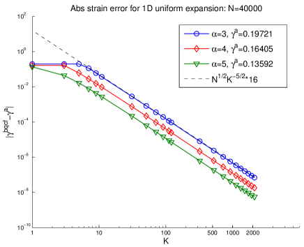
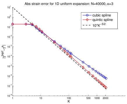
The computational results are shown in Figure 1. In Figure 1(a) we plot the dependence of the errors of quintic blending on $K$ for different values of $\alpha$. We see that the graph of the error for the quintic blending is very close to the lower bound $K^{-5/2}$ as given by (2.8) in Theorem 2.1. Also, the error is lower for larger $\alpha$, which is also in accordance with the theoretical results. Indeed, when $\alpha$ is large, the strength of the next-nearest neighbor interaction, $\phi^{\prime\prime}_{2F}$, is small relative to the nearest neighbor interaction $\phi^{\prime\prime}_{F}$, which contributes to a better stability of B-QCF according to (2.8).

Figure 1(b) shows the results of comparison of the cubic and the quintic blending. We see that the cubic blending produces the error that seems to decay slower, like $K^{-2}$. On the other hand, the quantitative difference between cubic and quintic is not large on the example considered. To observe a significantly higher accuracy of the quintic spline, the computational domain size $N$ has to be much larger. In addition, for larger $\alpha$, $N$ has to be even larger for the quintic blending to have advantage over the cubic blending.

(a) Quintic spline blending

(b) Quintic v.s. Cubic

Figure 1. (a) The absolute critical strain errors for a $1$D uniform expansion. We set $N=40,000,$ $\Delta\gamma=1/N^{2}$ where $\Delta\gamma$ is the strain increment used for testing stability, and $\gamma^{\rm{a}}$ and $\gamma^{\rm{bqcf}}$ are the critical strains for the atomistic and B-QCF models, respectively. The dashed line corresponds to the theoretical asymptote. (b) The absolute critical strain errors of quintic and cubic blending functions with $N=40,000$ and $\alpha=3$. The solid line corresponds to the theoretical asymptote.

3. The B-QCF Operator in $2$D.

3.1. The Triangular Lattice

For some integer $N\in\mathbb{N}$ and $\epsilon:=1/N$, we define the scaled 2D triangular lattice $\mathbb{L}$ to be

$$\mathbb{L}:=\mathtt{A}_{6}\mathbb{Z}^{2},\quad\text{where}\quad\mathtt{A}_{6}:=\left[{a}_{1},{a}_{2}\right]:=\epsilon\left[\begin{array}[]{cc}1&1/2\\ 0&\sqrt{3}/2\end{array}\right],$$

where ${a}_{i},\,i=1,2$ are the scaled lattice vectors. Throughout our analysis, we use the following definition of the periodic reference cell

$$\Omega:=\mathtt{A}_{6}(-N/2,N/2]^{2}\quad\text{and}\quad\mathcal{L}:=\mathbb{L}\cap\Omega.$$

We furthermore set ${a}_{3}=(-1/2\epsilon,\sqrt{3}/2\epsilon)^{\mathtt{T}}$, then the set of nearest-neighbor directions is given by

$$\mathcal{N}_{1}:=\{\pm{a}_{1},\pm{a}_{2},\pm{a}_{3}\}.$$

The set of next nearest-neighbor directions is given by

$$\mathcal{N}_{2}:=\{\pm{b}_{1},\pm{b}_{2},\pm{b}_{3}\},\quad\text{where}\quad b_{1}:=a_{1}+a_{2},\quad b_{2}:=a_{2}+a_{3},\quad\text{and}\quad b_{3}=a_{3}-a_{1}.$$

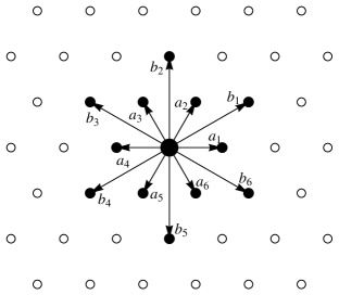
We use the notation $\mathcal{N}:=\mathcal{N}_{1}\cup\mathcal{N}_{2}$ to denote the directions of the neighboring bonds in the interaction range of each atom (see Figure 2).

We identify all lattice functions $\mathbf{v}:\mathbb{L}\to\mathbb{R}^{2}$ with their continuous, piecewise affine interpolants with respect to the canonical triangulation $\mathcal{T}$ of $\mathbb{R}^{2}$ with nodes $\mathbb{L}$.

(a) Neighbor set

(b) Domain decomposition

Figure 2. (a) The 12 neighboring bonds of each atom. (b) The periodic reference cell $\mathcal{L}:=\mathbb{L}\cap\Omega,$ the atomistic region $\Omega_{a}:=\mathtt{Hex}(\epsilon R_{a}),$ and the blending region $\Omega_{b}:=\mathtt{Hex}(\epsilon R_{b})\setminus\Omega_{a}$. Here, $N=32,$ $R_{a}=3$, $R_{b}=7$, and $K=4$.

3.2. The Atomistic, Continuum, and Blending Regions

Let $\mathtt{Hex}(R)$ denote the closed hexagon centered at the origin, with sides aligned with the lattice directions $a_{1},a_{2},a_{3}$, and diameter $2R$. For $R_{a}<R_{b}\ <N\in\mathbb{N}$, we define the atomistic, blending, and continuum regions, respectively, as

$$\Omega_{a}:=\mathtt{Hex}(\epsilon R_{a}),\quad\Omega_{b}:=\mathtt{Hex}(\epsilon R_{b})\setminus\Omega_{a},\quad\text{and}\quad\Omega_{c}:={\rm clos}\left(\Omega\setminus\left(\Omega_{a}\cup\Omega_{b}\right)\right).$$

We denote the blending width by $K:=R_{b}-R_{a}$. Moreover, we define the corresponding lattice sites

$$\mathcal{L}^{a}:=\mathcal{L}\cap\Omega_{a},\qquad\mathcal{L}^{b}:=\mathcal{L}\cap\Omega_{b},\qquad\text{and}\qquad\mathcal{L}^{c}:=\mathcal{L}\cap\Omega_{c}.$$

For simplicity, we will again use $\mathcal{L}$ as the finite element nodes, that is, every atom is a repatom. For a map $\mathbf{v}:\mathbb{L}\rightarrow\mathbb{R}^{2}$ and bond directions $r,s\in\mathcal{N}$, we define the finite difference operators

$$D_{r}v(x):=\frac{v(x+r)-v(x)}{\epsilon}\quad\text{and}\quad D_{r}D_{s}v(x):=\frac{D_{s}v(x+r)-D_{s}v(x)}{\epsilon}.$$

We define the space of all admissible displacements, $\mathcal{U}$, as all discrete functions $\mathbb{L}\rightarrow\mathbb{R}^{2}$ which are $\Omega$-periodic and satisfy the mean zero condition on the computational domain:

$$\mathcal{U}:=\Big{\{}\mathbf{u}:\mathbb{L}\rightarrow\mathbb{R}^{2}:\text{$u(x)$ is $\Omega$-periodic and }{\textstyle\sum_{x\in\mathcal{L}}}u(x)=0\Big{\}}.$$

For a given matrix $B\in\mathbb{R}^{2\times 2}$, $\mathrm{det}(B)>0$, we admit deformations $\mathbf{y}$ from the space

$$\mathcal{Y}_{B}:=\big{\{}\mathbf{y}:\mathbb{L}\rightarrow\mathbb{R}^{2}:y(x)=Bx+u(x){{\color[rgb]{0.0,0,0}\,\,\,\forall x\in\mathbb{L},\,}}\text{ for some $\mathbf{u}\in\mathcal{U}$}\big{\}}.$$

For a displacement $\mathbf{u}\in\mathcal{U}$ and its discrete directional derivatives, we employ the weighted discrete $\ell_{\epsilon}^{2}$ and $\ell_{\epsilon}^{\infty}$ norms given by

$$\|\mathbf{u}\|_{\ell_{\epsilon}^{2}}:=\left(\epsilon^{2}\sum_{x\in\mathcal{L}}|u(x)|^{2}\right)^{1/2},\quad\|\mathbf{u}\|_{\ell_{\epsilon}^{\infty}}:=\max\limits_{x\in\mathcal{L}}|u(x)|,\quad\text{and}$$

$$\qquad\quad\|D\mathbf{u}\|_{\ell_{\epsilon}^{2}}:=\left(\epsilon^{2}\sum_{x\in\mathcal{L}}\sum_{i=1}^{3}|D_{a_{i}}u(x)|^{2}\right)^{1/2}.$$

The inner product associated with $\ell^{2}_{\epsilon}$ is

$$\langle\mathbf{u},\mathbf{w}\rangle:=\epsilon^{2}\sum\limits_{x\in\mathcal{L}}u(x)\cdot w(x).$$

3.3. The B-QCF operator.

The total scaled atomistic energy for a periodic computational cell $\Omega$ is

$$\mathcal{E}^{\rm{a}}(\mathbf{y})= \frac{\epsilon^{2}}{2}\sum_{x\in\mathcal{L}}\sum_{r\in\mathcal{N}}\phi(D_{r}y({x}))=\epsilon^{2}\sum_{x\in\mathcal{L}}\sum_{i=1}^{3}\big{[}\phi(D_{a_{i}}y({x}))+\phi(D_{b_{i}}y({x}))\big{]},$$ (3.1)

where $\phi\in C^{2}(\mathbb{R}^{2})$, for the sake of simplicity. Typically, one assumes $\phi(r)=\varphi(|r|)$; the more general form we use gives rise to a simplified notation; see also [33]. We define $\phi^{\prime}(r)\in\mathbb{R}^{2}$ and $\phi^{\prime\prime}(r)\in\mathbb{R}^{2\times 2}$ to be, respectively, the gradient and hessian of $\phi$.

The equilibrium equations are given by the force balance at each atom,

$$F^{a}(x;y)+f(x;y)=0,\quad\text{for}\quad x\in\mathcal{L},$$ (3.2)

where $f(x;y)$ are the external forces and $F^{a}(x;y)$ are the atomistic forces (per unit area $\epsilon^{2}$)

$$F^{\rm a}(x;y):= -\frac{1}{\epsilon^{2}}\frac{\partial\mathcal{E}^{\rm a}(\mathbf{y})}{\partial y(x)}$$

$$= -\frac{1}{\epsilon}\sum_{i=1}^{3}\Big{[}\phi^{\prime}\left(D_{a_{i}}y(x)\right)+\phi^{\prime}\left(D_{-a_{i}}y(x)\right)\Big{]}-\frac{1}{\epsilon}\sum_{i=1}^{3}\Big{[}\phi^{\prime}\left(D_{b_{i}}y(x)\right)+\phi^{\prime}\left(D_{-b_{i}}y(x)\right)\Big{]}.$$

Again, since $\mathbf{u}=\mathbf{y}-\mathbf{y}_{B}$, where $y_{B}(x)=Bx$, is assumed to be small, we linearize the atomistic equilibrium equation (3.2) about $\mathbf{y}_{B}$:

$$\left(L^{\rm a}\mathbf{u}^{\rm a}\right)(x)=f(x),\quad\text{for}\quad x\in\mathcal{L},$$

where $\left(L^{\rm a}\mathbf{u}\right)(x)$, for a displacement $\mathbf{u}$, is given by

$$\left(L^{\rm a}\mathbf{u}\right)(x)=-\sum_{i=1}^{3}\phi^{\prime\prime}(Ba_{i})D_{a_{i}}D_{a_{i}}u(x-a_{i})-\sum_{i=1}^{3}\phi^{\prime\prime}(Bb_{i})D_{b_{i}}D_{b_{i}}u(x-b_{i}),\quad\text{for}\quad x\in\mathcal{L}.$$

We use the Cauchy-Born extrapolation rule to approximate the nonlocal atomistic model by a local continuum Cauchy-Born model [41, 39, 29]. Using the bond density lemma [33, Lemma 3.2] (see also [37]), we can write the total QCL energy (the discretized Cauchy-Born energy) as a sum of the bond density integrals

$$\mathcal{E}^{\rm c}(\mathbf{y})={{\color[rgb]{0.0,0,0}\frac{1}{\Omega_{0}}}}\int_{\Omega}\sum_{r\in\mathcal{N}}\phi(\partial_{r}y)\,dx=\sum_{x\in\mathcal{L}}\sum_{r\in\mathcal{N}}\int_{0}^{1}\phi\big{(}\partial_{r}y(x+tr)\big{)}dt,$$ (3.3)

where the factor $\Omega_{0}:=\sqrt{3}/2$ is the volume of one primitive cell of $\mathcal{L}$ and $\partial_{r}y(x):=\frac{d}{dt}y(x+tr)|_{t=0}$ denotes the directional derivative. We compute the continuum force

$$F^{\rm c}(x;y)=-\frac{1}{\epsilon^{2}}\frac{\partial\mathcal{E}^{\rm c}}{\partial y(x)},$$

and linearize the force equation about the uniform deformation $\mathbf{y}_{B}$ to obtain

$$\left(L^{\rm c}\mathbf{u}^{\rm c}\right)(x)=f(x),\quad\text{for}\quad x\in\mathcal{L}.$$

To formulate the B-QCF method, we let the blending function $\beta(s):\mathbb{R}^{2}\rightarrow[0,1]$ be a “smooth”, $\Omega$-periodic function. Then, the (nonlinear) B-QCF forces are given through a convex combination of $F^{\rm a}(x;y)$ and $F^{\rm c}(x;y)$:

$$F^{\rm{bqcf}}(x;y):=\beta(x)F^{\rm a}(x;y)+(1-\beta(x))F^{\rm c}(x;y),$$

and linearizing the equilibrium equation $F^{\rm{bqcf}}+f=0$ about $y_{B}$ yields

$$\begin{split}&(L^{\rm{bqcf}}\mathbf{u}^{\rm{bqcf}})(x)=f(x),\quad\text{for }x\in\mathcal{L},\\ &\text{where}\quad(L^{\rm{bqcf}}\mathbf{u})(x)=\beta(x)(L^{\rm a}\mathbf{u})(x)+(1-\beta(x))(L^{\rm c}\mathbf{u})(x).\end{split}$$ (3.4)

The $2$D blending function in our computational experiments will be defined radially using cubic and quintic splines:

$$\hat{\beta}(x):=\hat{B}\left(\frac{\epsilon R_{b}-|x|}{\epsilon R_{b}-\epsilon R_{a}}\right)\quad\text{ and }\quad\bar{\beta}(x):=\bar{B}\left(\frac{\epsilon R_{b}-|x|}{\epsilon R_{b}-\epsilon R_{a}}\right),$$

where $\hat{B}(x)$ is given by (2.10) and $\bar{B}(x)$ is given by (2.11). The function $\bar{\beta}(x)$ has the smoothness and satisfies 2D versions of the scaling bounds (2.5) needed for Theorem 3.1 below, whereas $\hat{\beta}(x)$ does not have a bounded third derivative. We therefore can expect that $\hat{\beta}(x)$ will give a larger error asymptotically as compared to $\bar{\beta}(x)$.

3.4. Positivity of the B-QCF operator in 2D

Necessary and sufficient conditions for $L^{\rm{bqcf}}$ to be positive-definite are given in [21]. To make this paper more concise, we only state the conclusions without proof. First, we state a lower bound for $\langle L^{\rm{bqcf}}\mathbf{u},\mathbf{u}\rangle$:

Theorem 3.1.

Suppose that $\beta\in C^{3}$ and satisfies the scaling bounds (2.5); then,

$$\langle L^{\rm{bqcf}}\mathbf{u},\mathbf{u}\rangle\geq\gamma_{\rm{bqcf}}\|D\mathbf{u}\|_{\ell^{2}_{\epsilon}}^{2},$$

where

$$\gamma_{\rm{bqcf}}:=\tilde{\gamma}-C\,\big{[}K^{-5/2}R_{b}^{1/2}|\log(R_{b}/N)|^{1/2}\big{]},$$ (3.5)

where $C$ is a generic constant independent of $N$, and $\tilde{\gamma}$ is the coercivity constant for the operator $\tilde{L}$:

$$\langle\tilde{L}\mathbf{u},\mathbf{u}\rangle:=\langle L^{\rm c}\mathbf{u},\mathbf{u}\rangle-\epsilon^{4}\sum_{i=1}^{3}\sum_{x\in\mathcal{L}}\beta(x-a_{2})\big{|}D_{a_{i}}D_{a_{i+1}}u(x-a_{1}-a_{2})\big{|}_{b_{i}}^{2}\geq\tilde{\gamma}\|D\mathbf{u}\|_{\ell^{2}_{\epsilon}}^{2}\qquad\forall\mathbf{u}\in\mathcal{U}.$$

One can see very clearly that, whenever $N$ is polynomial in $R_{b}$ and $K\gg R_{b}^{1/5}$, then $L^{\rm bqcf}$ can be expected to be coercive. Both are natural and easy to achieve. We can thus deduce the following result for the coercivity of $L^{\rm{bqcf}}:$

Corollary 3.1.

Suppose that $\tilde{L}$ is positive-definite and that the blending function $\beta\in C^{3}$ and satisfies the scaling bounds (2.5). Let the number of atoms $R_{a}$ along the radius be of order $N^{\alpha}$ with $0\leq\alpha\leq 1$. If the blending width $K$ satisfies

$$K\gg\begin{cases}|\log{N}|^{1/4},\quad\alpha=0,\\ |\log{N}|^{1/5}N^{\alpha/5},\quad 0<\alpha<1,\\ N^{1/5},\quad\alpha=1,\end{cases}$$

then the B-QCF operator $L^{\rm{bqcf}}$ is positive-definite.

Remark 3.1.

• The stability result of Theorem 3.1, and hence of Corollary 3.1, is based on the conjecture that the operator $\tilde{L}$ is stable. In [21] we show that $\tilde{L}$ is indeed stable whenever nearest-neighbor interactions dominate.

  Moreover, based on the analysis and numerical experiments in [33] for a similar linearized operator, we expect that the region of stability for $\tilde{L}$ is the same as for $L^{a}$ as $N,\,R_{a},\,R_{b}\rightarrow\infty$. We therefore expect that the result of Theorem 3.1 holds (up to a controllable error) if coercivity of $\tilde{L}$ is replaced by coercivity of $L^{\rm{a}}$ in the hypothesis.

• One can apply the argument of Remark 2.1 to conclude that the results of Theorem 3.1 and Corollary 3.1 are valid for homogeneous Dirichlet boundary conditions as well.

By constructing a radial counterexample similar to our $1$D counterexample, we can observe that our conditions in Corollary 3.1 are essentially necessary.

Theorem 3.2.

Suppose that $L^{\rm a}$ is positive-definite and that the blending function $\beta\in C^{3}$ and satisfies the scaling bounds (2.5). The number of atoms $R_{a}$ along the radius is of order $N^{\alpha}$ with $0<\alpha\leq 1$. If the blending width $K$ is $K\ll N^{\alpha/5}$, then the B-QCF operator $L^{\rm{bqcf}}$ cannot be positive-definite and we can construct a radial counterexample in this case.

We note that there is a gap between the necessary and sufficient conditions for $0<\alpha<1$. In addition, we have no necessary condition for $\alpha=0$, which corresponds to a fixed atomistic core independent of the reference cell $\Omega$.

3.5. 2D numerical experiments for B-QCF operators.

In this subsection, we will continue the numerical experiments for the $2$D B-QCF models to verify the theoretical findings by comparing the decay rates of the error in critical strain as computed by B-QCF with the theoretically predicted rates as we increase the blending width $K$.

1. Uniform expansion.

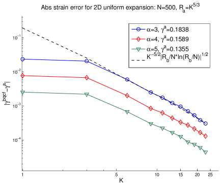
   We first consider the simplest $2$D deformation: we apply a uniform expansion $y(x)=Bx$ with

   $$B=\gamma\left(\begin{array}[]{cc}1&0\\ 0&1\end{array}\right)$$

   to the perfect lattice $\mathcal{L}$ with Dirichlet boundary condition:

   $$u(x)=0\quad\forall x\in\partial\Omega.$$ (3.6)

   Then we compute the critical strains $\gamma$ of the atomistic and B-QCF models with different blending region width $K$.

   We note that the $2$D conclusions also depend on the size of the atomistic region. Therefore we let $R_{a}=K^{5/3}$ in order to narrow the dependence only to the blending width $K$. Then the asymptotical term in (3.5) for sufficiently large $N$ is approximately

   $$K^{-5/2}R_{b}^{1/2}|\log(R_{b}/N)|^{1/2}= K^{-5/2}(R_{a}+K)^{1/2}|\log(R_{b}/N)|^{1/2}$$

   $$\approx K^{-5/2}R_{a}^{1/2}=K^{-5/3}=R_{a}^{-1},$$

   which means that the error in $\gamma_{\rm{bqcf}}$ is systematically improvable.

   The choice of scaling $R_{a}=K^{5/3}$ is motivated by the results in [17] which indicate that, generically, one should expect an $O(R_{a}^{-1})$ error in the regions of stability between the infinite lattice atomistic model and the atomistic model in a domain with radius $R_{a}$. In the computation, we assign integer values for $K$ and use the rounded values for $R_{a}$, that is $R_{a}=\lfloor K^{5/3}\rfloor$.

   The critical strains are defined as

   $$\gamma^{\rm w}:=\max\big{\{}\bar{\gamma}>0:L^{\rm w}(B\mathbf{x})\text{ is positive definite for }\gamma\in[0,\bar{\gamma})\big{\}},$$ (3.7)

   where $\rm{w}\in\{\rm a,\rm{bqcf}\}$ denote the models. Here we use the MATLAB function eigs [28] to compute the smallest eigenvalue of the symmetric part of $L^{\rm w}(B\mathbf{x})$ and thus determine the positive-definiteness of $L^{\rm w}(B\mathbf{x})$.

   We also define the increment of the strain $\gamma$ in each step by $\Delta\gamma$. The results in [33, 17, 14, 10] suggest that the theoretical increments be of order $O(N^{-2})$ (at least, for finding the critical strain of a uniform lattice), and we set $\Delta\gamma=10^{-8}$ which is sufficiently small considering $N=200$ or $300$ in our experiments.

   

   (a) Quintic spline blending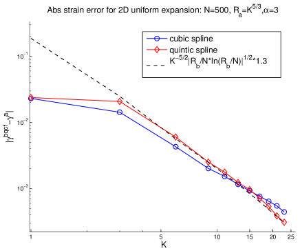

   

   (b) Quintic v.s. Cubic

   Figure 3. (a) The absolute critical strain errors for the $2$D uniform expansion. We set $N=500$, and we denote the critical strains for the atomistic and B-QCF models by $\gamma^{\rm a}$ and $\gamma^{\rm{bqcf}},$ respectively. The dashed line corresponds to the theoretical asymptote. (b) The absolute critical strain errors for the quintic and cubic blending functions with $N=500$ and $\alpha=3$. The solid line corresponds to the theoretical asymptote.

   We plot the difference of the critical strains with different blending width $K$ in Figure 3. The numerical critical strain errors in the left figure approach the analytical asymptote as $K$ increases. There are larger fluctuations of errors as compared to the $1$D case, which is likely due to round-off errors in calculating $R_{a}=K^{5/3}$. Thus, the slopes of the errors with quintic blending agree with the theoretical prediction in Theorem 3.1. Also, similarly to the 1D results, the error is smaller when the nearest neighbor interaction dominates (that is, when $\alpha$ is large).

   Although the slope of the errors with cubic blending seems to be one half order less than that with quintic blending (see Figure 3(b)), the computed errors for cubic blending are slightly smaller for the relatively small $N$ considered. We expect that for a sufficiently large system, the quintic blending would be more accurate. In addition, the $2$D errors for uniform expansion are similar to the $1$D results. This is reasonable since the $2$D uniform expansion is similar to the $1$D deformation.

2. Uniform shear deformation.

   We now investigate stability of B-QCF under shear deformation. We apply a y-directional shear deformation to the hexagonal lattice $\Omega$ with Dirichlet boundary conditions (3.6). The y-directional shear is $y(x)=\tilde{B}x$ with

   $$\tilde{B}=\left(\begin{array}[]{cc}1&0\\ \gamma&1\end{array}\right).$$

   The critical strain errors between the B-QCF and atomistic models with the quintic blending are plotted in Figure 4.

   

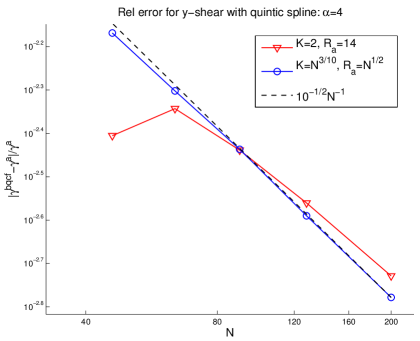
   (a) Error vs 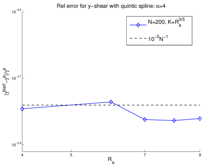$N$

   

   (b) Error vs $R_{a}$

   Figure 4. The relative critical strain error for the y-directional shear deformation. $\gamma^{\rm a}$ and $\gamma^{\rm{bqcf}}$ are the critical strains for the atomistic and B-QCF models respectively. For $N=200$, $\gamma^{a}\approx 0.1813.$ The dashed line corresponds to the theoretical asymptote. The fluctuations in the plotted error for $N={\rm const}$ seems to be due to round-off errors in calculating $R_{a}$ and $K$. The method parameters were rounded as follows: in (a) $K=\lfloor N^{3/10}\rfloor$ and $R_{a}=\lfloor N^{1/2}\rfloor$, and in (b) $K=\lfloor R_{a}^{3/5}\rfloor$.

   In Figure 4 we plot the critical strain errors in the following three regimes: (1) $N$ increases, $R_{a}={\rm const}$, $K={\rm const}$, (2) all three parameters increase, and (3) $N={\rm const}$, $R_{a}$ and $K$ increases. The choice of constant parameters, $K=2$ and $R_{a}=14$, does not follow the scaling $K\approx R_{a}^{3/5}$, and was made to show that such nonoptimal parameters do not significantly affect the results in this case. The results indicate that the error in this case depends on $N$, but does not depend on $R_{a}$ or $K$. This means that, for shear deformations, the local continuum approximation and its finite element coarse-graining contributes most of the error.

   We explain such a qualitative difference between the uniform expansion and the shear deformation in the following way. For the uniform expansion the onset of instability is due to competition of interaction of the nearest neighbors (NNs), contributing to stability, and the second nearest neighbors (NNNs), contributing to instability. On the other hand, for the shear deformation the onset of instability is primarily due to competition between elongated and compressed NN bonds. Therefore, for the uniform expansion it is important to reduce the interface error which distorts the NNN interaction, whereas in shear deformation the NNN interactions do not contribute significantly to stability errors. Since, for NN interaction, the atomistic, Cauchy-Born and B-QCF models are identical, the stability error only depends on the domain size.

3. Regions of stability.

   We now combine the uniform expansion and shear deformation together and study the stability region of $L^{\rm{bqcf}}$ for a general class of homogeneous deformations. We consider the following family of deformations which involve shear, expansion, and compression.

   $$B=\left(\begin{array}[]{cc}1+s&0.1\\ 0&1+r\end{array}\right).$$

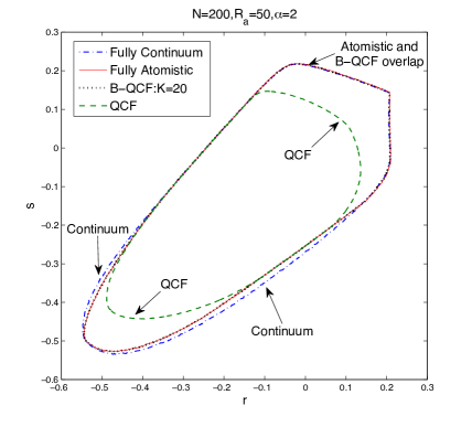
   Applying these specific homogeneous deformations to the hexagonal lattice in the reference cell and again using the Dirichlet boundary condition, we plot the stability regions (regions where the operators are positive definite) in Figure LABEL:StabRegRa50Fig1.

   

   (a) 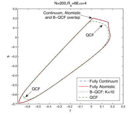$\alpha=2$

   

   (b) $\alpha=4$

   Figure 5. The stability regions of the different models. These closed curves are the boundaries of the stability regions for the atomistic, B-QCF, and the local continuum models, respectively. The curves with indicators are for QCF.

   We observe that the stability regions of the B-QCF model with different blending sizes are all proper subsets of the atomistic model. In addition, the fully atomistic and continuum models are very close to each other, which agrees with the stability analysis of the perfect lattice [17]. Also, when $\alpha$ increases, which means the next-nearest neighbor interactions become less important, the difference becomes smaller.

   There is a visible difference in the stability regions between the QCF model and the exact atomistic model, whereas the difference between the B-QCF model and the atomistic model is almost not seen. This implies that using a blending region can significantly improve the stability properties of the approximation models.

4. Stability of micro-cracks.

   The experiments that we have reported up to this point were based on perfect lattices. Now we apply the B-QCF model to lattices with local defects.

   The atomistic system is as follows. There is a micro-crack in the center of the domain $\Omega$ with length $5$, i.e., $5$ atoms are removed from the lattice (see Figure 6). Hence, we redefine accordingly the positions of atoms in the reference configuration $\mathbf{x}$, the interaction energy $\mathcal{E}^{a}$, etc. We impose a vertical stretching $B=\left[\begin{array}[]{cc}1&0\\ 0&1+\gamma\end{array}\right]$ on the lattice and compute the critical strains $\gamma^{\rm c}>0$ beyond which the system loses stability.

   

   Figure 6. The stable equilibrium configuration of the micro-crack with crack length$=5$ and $\gamma=0.001$, and the $\ell^{\infty}_{\epsilon}$ norm of the force residual is of order $O(10^{-12}).$

   We computed the critical strain $\gamma^{\rm c}$ in the following way. Given $\gamma>0$, we use Newton’s iteration method to solve the following force equations for $\mathbf{y}^{\gamma}$ with the initial guess $\mathbf{y}_{F}=B\mathbf{x}$:

   $$F^{w}(x;y^{\gamma})=0\quad\text{for}\quad x\in\Omega\setminus\partial\Omega.$$

   We set the tolerance for the $\ell^{\infty}_{\epsilon}$ norm of the force residual of the Newton’s iteration to be $10^{-5}$. To prevent the configuration from “jumping out” of the local energy well corresponding to the defect under consideration, we require at each step the $\ell_{\epsilon}^{\infty}$ norm of force residual to be less than $100$ and the positive-definiteness of $L^{w}(\mathbf{y})$, where $\mathbf{y}$ is the current configuration. If any of the two requirements is not met, then the current $\gamma$ is regarded as an unstable strain. When the force residual is smaller than the tolerance, the configuration $\mathbf{y}^{*}$ is thought to be in its equilibrium of the local energy well. Then we check the positive definiteness of corresponding operator $L^{\rm{w}}(\mathbf{y}^{*})$ with the equilibrium configuration $\mathbf{y}^{*}$. The nonlinear critical strain is thus defined as

   $$\gamma^{\rm c}:=\max\{\bar{\gamma}>0:L^{\rm{w}}(\mathbf{y}^{*})\text{ is positive definite for }\gamma\in[0,\,\bar{\gamma})\}.$$

   The plot of critical strain for the B-QCF models are shown in Figure 7.

   

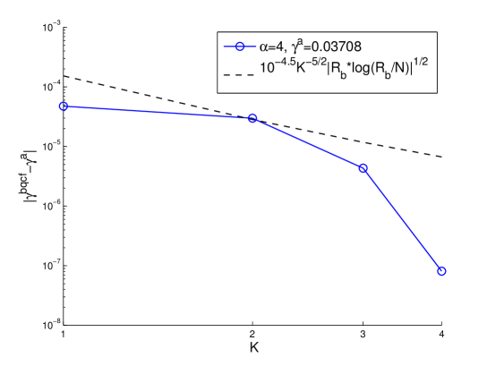
   Figure 7. The nonlinear critical strain error for vertical stretching. We set $N=200$, crack length$=5$, and $R_{a}=\max\{K^{2},6\}$. $\gamma^{\rm{a}}$, $\gamma^{\rm{bqcf}}$ are the critical strains for the atomistic and B-QCF models, respectively. The dashed line corresponds to the theoretical asymptote.

   Even though we choose the blending width $K\approx R^{1/2}$ slightly smaller then our previous choice ($K\approx R^{3/5}$), we observe the nonlinear error decays much faster than the theoretical predicted rates and it can reach the strain increment $\Delta\gamma=10^{-8}$. This phenomenon has been observed in [33] and is likely related to superconvergence of local quantities of interest. The indicator of the superconvergence is the concentration of the critical eigenmode corresponding to $\gamma^{\rm c}$ near the defect, which is illustrated in Figure 8.

   

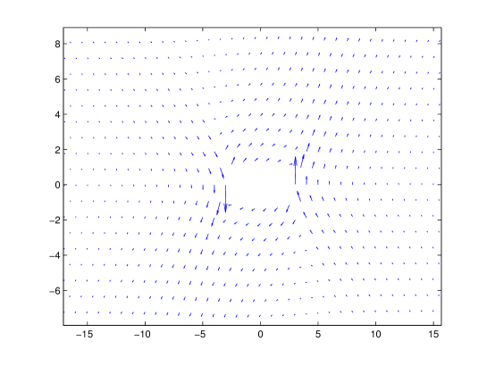
   Figure 8. The zoomed-in critical eigenvector of critical strain of vertically stretching a micro-crack. We set $N=200$, crack length$=5$, strain increment $\Delta\gamma=10^{-11}$ and $\alpha=4.$

   We also study the relative errors of the critical strains for two different choices of the blending width, $K=2$ and $K\approx R_{a}^{3/5}+2$. Motivated by the analysis in [33], the size of the atomistic core is chosen to be $R_{a}=\sqrt{N}$. According to Figure 9, the relative errors for $K\approx R_{a}^{3/5}+2$ are approximately $10$ times smaller than those for $K=2$. But both graphs decay rapidly as $N$ increases. The rate of decay appears to be quadratic.

   

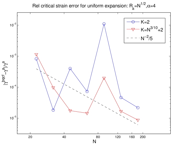
   Figure 9. The relative errors of the critical strains of vertically stretching a micro-crack in $\log_{10}$ scale plot. We set crack length$=5$ and $\alpha=4$. $\gamma^{\rm a}$, $\gamma^{\rm{bqcf}}$ are the critical strains for the atomistic and B-QCF models, respectively. The dashed line is the theoretical asymptote.

Remark 3.2.

The numerical computations in this section are conducted without coarsening. The main reason for this was that coarsening introduces more approximation parameters and potentially more fluctuations in the results. Typically, coarsening does not reduce the stability, and we therefore expect that our stability results will remain valid for any coarsening. Another reason to discard coarsening was to better compare the numerics with the theory. However, the purpose of a/c coupling is to reduce the number of degrees of freedom of an atomistic computation, therefore coarsening is required when comparing efficiency (i.e., accuracy against the number of degrees of freedom) of different methods.

4. The Accuracy of B-QCF

In the previous sections, we investigated the positivity of the B-QCF operator. One motivation for this study is that these experiments fill a gap in our error analysis of the B-QCF method [19]. We now briefly review these results and then include some numerical experiments demonstrating the superior accuracy of B-QCF over other a/c coupling schemes that we have investigated previously in [27].

4.1. Implementation of the B-QCF method

Let $\mathcal{V}\subset\mathbb{L}$ be a set of vacancy sites and $\mathbb{L}_{\mathcal{V}}:=\mathbb{L}\setminus\mathcal{V}$ the corresponding lattice with defects. Let $B\in\mathbb{R}^{2\times 2}$ be the applied far-field strain. We consider the atomistic problem

$$y^{\rm a}\in\arg\min\big{\{}\mathcal{E}^{\rm a}(y):y:\mathbb{L}_{\mathcal{V}}\to\mathbb{R}^{2},y(x)\sim Bx\text{ as }|\xi|\to\infty\big{\}}.$$ (4.1)

We remark that one must carefully renormalize $\mathcal{E}^{\rm a}$ in order to rigorously make sense of this problem; see e.g. [19] for the details. The vacancy sites are accounted for in the definition of $\mathcal{E}^{\rm a}$ by simply removing the relevant pair interactions.

We wish to approximate this problem with a practical variant (i.e., with coarsening) of the B-QCF method. To that end, we choose $R_{a},R_{b}=R_{a}+K,N\in\mathbb{N}$ in such a way that all vacancy sites are contained in the atomistic region $\Omega_{a}$, which is a hexagon with side length $R_{a}$. The blending region is defined analogously. The full computational domain is given by $\Omega$, which is a hexagon with side length $N$. We triangulate $\Omega$ in such a way that it matches the canonical triangulation of the triangular lattice in $\Omega$.

Let $\mathcal{T}_{h}$ denote the set of triangles, let $\mathcal{N}_{h}$ denote the nodes of the triangulation, and let $\mathcal{N}_{h}^{\rm free}:=\mathcal{N}_{h}\setminus(\mathcal{V}\cup\partial\Omega)$ denote the free nodes.

Let ${\rm P}^{1}_{h}$ denote the space of all functions $v_{h}:\Omega\to\mathbb{R}^{2}$, that are continuous and piecewise affine with respect to the triangulation $\mathcal{T}_{h}$. The space of admissible trial functions is then given by

$${\rm Y}_{h}:=\big{\{}y_{h}\in{\rm P}^{1}_{h}:y_{h}(x)=Bx\text{ for }x\in\partial\Omega\big{\}}.$$

Each deformation $y_{h}\in{\rm Y}_{h}$ is understood to be extended by $Bx$ outside of $\Omega$ and thereby gives rise to an admissible atomistic configuration.

We define the discretized Cauchy-Born energy functional as

$$\mathcal{E}^{\rm c}(y_{h}):=\sum_{T\in\mathcal{T}_{h}}{\rm vol}(T)W\big{(}\nabla y_{h}|_{T}\big{)},$$

where ${\rm vol}(T)$ in $2$D is the area of the triangle $T$. We can define the discretized B-QCF operator, for a given blending function $\beta$, as follows:

$$F^{\rm bqcf}(x;y_{h}):=(1-\beta(x))\frac{\partial\mathcal{E}^{\rm a}(y)}{\partial y(x)}\Big{|}_{y=y_{h}}+\beta(x)\frac{\partial\mathcal{E}^{\rm c}(z_{h})}{\partial z_{h}(x)}\Big{|}_{z_{h}=y_{h}}\qquad\text{ for }x\in\mathcal{N}_{h}^{\rm free}.$$

In the B-QCF method, we aim to find a solution $y_{h}^{\rm bqcf}\in{\rm Y}_{h}$ satisfying

$$F^{\rm bqcf}(x;y_{h}^{\rm bqcf})=0\qquad\forall x\in\mathcal{N}_{h}^{\rm free}.$$ (4.2)

We remark that this method has essentially five approximation parameters that must be chosen carefully: the atomistic region size $R_{a}$, the blending width $K$, the computational domain size $N$, the blending function $\beta,$ and the finite element mesh $\mathcal{T}_{h}$.

4.1.1. Practical considerations

To implement (4.2) in practice, we need to specify further details of the method:

1. In our choice of blending function, we deviate from the optimal choice of a $C^{2,1}$-blending function and instead choose only a $C^{1,1}$ blending function, which is more easily constructed. This is justified, firstly, by our foregoing numerical experiments which suggest that little additional accuracy in the stability regions can be gained in the pre-asymptotic regime by using quintic splines (i.e., $C^{2,1}$-blending), and secondly, because the consistency error does not depend on the regularity of the blending function.

   We choose the blending function proposed in [27], which minimizes $\|\nabla^{2}\beta\|_{L^{2}}$, or a discrete variant thereof, in a precomputation step (see [27] for the details).

2. In addition to the blending region $\Omega_{b}$ we ensure that two additional “layers” of atoms outside of it belong to $\mathcal{N}_{h}$. This makes the implementation of the atomistic force contribution in (4.2) straightforward.

   Moreover, we ensure that the vacancy sites do not affect the forces on atoms $x$ where $\beta(x)\neq 0$. This ensures that all the Cauchy-Born force contributions in (4.2) are the correct Cauchy-Born forces.

3. To obtain an appropriate initial guess for the B-QCF solutions, we first solve the corresponding energy-based blended QCE method (B-QCE) [27] with the same approximation parameters, using a preconditioned line search method. The details are described in [27]. The B-QCE solution is then taken as a starting guess for the B-QCF Newton iteration to solve (4.2). If no B-QCE code is readily available, then a natural alternative would be to implement a damped Newton method for B-QCF.

   We remark, that the Jacobian matrix of the B-QCF operator is straightforward to assemble from the Hessians of the atomistic and Cauchy-Born energy. Nevertheless, for large 3D simulations, more sophisticated solution methods may be required.

4. We are now only left to choose the remaining approximation parameters $R_{a},K,N$ and the mesh $\mathcal{T}_{h}$.

4.2. Error versus computational cost

We briefly review the main ideas of our analysis in [19] without technical details. A first key result is that if the atomistic solution is stable ($\delta^{2}\mathcal{E}^{\rm a}(y^{\rm a})$ is positive definite) and the linearized B-QCF operator $\delta F^{\rm bqcf}(\cdot;Bx)$ is positive definite, then choosing $R_{a}$ and $K$ sufficiently large implies that $\delta F^{\rm bqcf}(\cdot;y^{\rm a})$ is also positive definite, that is, the B-QCF method is stable under these conditions. To achieve this in practice, we need to choose $K^{3}\gg R_{a}$ (recall from section 4.1.1 that we have chosen a sub-optimal $\beta$).

From this stability result, we can deduce the existence of a B-QCF solution in a neighborhood of the atomistic solution, and an error estimate in terms of the best approximation error (the best approximation of $y^{\rm a}$ from the finite element space ${\rm Y}_{h}$). and of the modeling error (the force discrepancy of the B-QCF and atomistic models). We estimate the error in the strain $\nabla y^{\rm a}-\nabla y_{h}^{\rm bqcf}$ in terms of the “smoothness” of $y^{\rm a}$, which is measured in terms of bounds on the derivatives $\nabla^{j}y^{\rm a}$. The derivatives of the discrete functions $y^{\rm a}$ are understood as derivatives of a smooth interpolant. (See [19] for the details.)

Dropping an unimportant term for the sake of readability, our error estimate reads

$$\|\nabla y^{\rm a}-\nabla y_{h}^{\rm bqcf}\|_{L^{2}(\mathbb{R}^{2})}\lesssim C^{\rm stab}\Big{(}C^{\beta}\|\nabla^{3}y^{\rm a}\|_{L^{2}(\mathbb{R}^{2}\setminus\omega_{\rm a})}+\|h\nabla^{2}y^{\rm a}\|_{L^{2}(\Omega\setminus\omega_{\rm a})}+\|\nabla y^{\rm a}\|_{L^{2}(\mathbb{R}^{2}\setminus\omega)}\Big{)},$$ (4.3)

where $\|\nabla^{3}y^{\rm a}\|_{L^{2}(\mathbb{R}^{2}\setminus\omega_{\rm a})}$ measures the modeling error, $\|h\nabla^{2}y^{\rm a}\|_{L^{2}(\Omega\setminus\omega_{\rm a})}$ the finite element discretization error and $\|\nabla y^{\rm a}\|_{L^{2}(\mathbb{R}^{2}\setminus\omega)}$ the error in the far-field due to the artificial boundary condition (the two latter errors comprise the best approximation error). The domains $\omega_{\rm a},\omega$ are slightly smaller hexagonal subsets of, respectively, $\Omega_{\rm a}$ and $\Omega$, with comparable side lengths.

In addition, $C^{\rm stab}$ is a stability constant that is uniformly bounded for $R_{a}\ll K^{3}$, and

$$C^{\beta}:=K^{-1/2}R_{a}^{1/2}\log\big{|}R_{a}/N\big{|}$$

is a $\beta$-dependent prefactor, which arises from a crucial inequality, $\|\nabla(\beta v)\|_{L^{2}}\leq C^{\beta}\|\nabla v\|_{L^{2}}$, in the consistency analysis of B-QCF.

We choose $K\approx R_{a}$ and $N$ a polynomial of $R_{a}$ (we will see momentarily why this is natural), then $C^{\beta}$ is uniformly bounded and in addition, we choose $R_{a}\ll K^{3}$ , which we require for stability. With this choice, it is easy to see that $C^{\beta}\|\nabla^{3}y^{\rm a}\|_{L^{2}(\mathbb{R}^{2}\setminus\omega_{\rm a})}\lesssim\|h\nabla^{2}y^{\rm a}\|_{L^{2}(\Omega\setminus\omega_{\rm a})}$ (recall that we are working in units where atomic spacing is $1$), and hence we can simply ignore the modeling error term from now on.

We recall from [27] that the atomistic method (ATM) is given by the B-QCF method with $\beta\equiv 0.$ We also recall the corresponding error estimates (dropping less important terms) for the atomistic (ATM) and the B-QCE methods [19, 27]

$$\|\nabla y^{\rm a}-\nabla y^{\rm atm}\|_{L^{2}(\mathbb{R}^{2})} \lesssim\|\nabla y^{\rm a}\|_{L^{2}(\mathbb{R}^{2}\setminus\omega)},$$ (4.4)

$$\|\nabla y^{\rm a}-\nabla y_{h}^{\rm bqce}\|_{L^{2}(\mathbb{R}^{2})} \lesssim\|\nabla^{2}\beta\|_{L^{2}(\mathbb{R}^{2}\setminus\omega_{\rm a})}+\|h\nabla^{2}y^{\rm a}\|_{L^{2}(\Omega\setminus\omega_{\rm a})}+\|\nabla y^{\rm a}\|_{L^{2}(\mathbb{R}^{2}\setminus\omega)}.$$ (4.5)

To better understand the best approximation error, we need to understand the regularity of $y^{\rm a}$. Since the problems only involve defects with zero Burgers vector, it is reasonable to assume based on linear elasticity, that

$$|\nabla^{j}y^{\rm a}(x)|\sim|x|^{-j-1}.$$

(We stress that this estimate only applies in the far-field. In the preasymptotic regime different rates of decay might be observed, e.g., $|\nabla^{j}y^{\rm a}(x)|\sim|x|^{1/2-j}$ for the micro-crack case discussed in § 4.3.2.)

Having this explicit knowledge about the elastic field, we can optimize our choice of finite element triangulation. Using the construction in [33] and also used successfully in our B-QCE experiments in [27], we obtain a triangulation $\mathcal{T}_{h}$ (as a function of $R_{b}$ and $N$), for which the following estimate holds:

$$\|h\nabla^{2}y^{\rm a}\|_{L^{2}(\Omega\setminus\omega_{\rm a})}+\|\nabla y^{\rm a}\|_{L^{2}(\mathbb{R}^{2}\setminus\omega)}\lesssim R_{a}^{-2}+N^{-1}.$$

Thus, we choose $N\approx R_{a}^{2}$ to balance these two error contributions.

Finally, we note that, with this construction, the number of degrees of freedom in ${\rm Y}_{h}$, ${\rm DoF}:={\rm dim}{\rm Y}_{h}=2\#\mathcal{N}_{h}^{\rm free}$ is approximately equal to ${\rm DoF}\approx R_{a}^{2}$. (In particular, the number of degrees of freedom in the atomistic, blending and continuum regions are comparable.)

In summary, choosing $K\approx R_{a},N\approx R_{a}^{2}$, the blending function $\beta$ according to the construction proposed in [27], and the finite element mesh according to the construction proposed in [33], we obtain from (4.3) the error estimate

$$\|\nabla y^{\rm a}-\nabla y_{h}^{\rm bqcf}\|_{L^{2}(\mathbb{R}^{2})}\lesssim{\rm DoF}^{-1}.$$ (4.6)

We note that $N=R_{a}$ in the ATM method, and consequently we obtain from (4.5)

$$\|\nabla y^{\rm a}-\nabla y^{\rm atm}\|_{L^{2}(\mathbb{R}^{2})}\lesssim{\rm DoF}^{-1/2};$$ (4.7)

thus demonstrating an improved rate of convergence for the B-QCF method in comparison with the ATM method.

We remark that this is optimal for P1-finite element type coarse-graining schemes, as the modeling error is in fact dominated by the finite element error. In particular, it is a substantial improvement over the B-QCE method, for which the corresponding error estimate obtained from (4.4) is

$$\|\nabla y^{\rm a}-\nabla y_{h}^{\rm bqce}\|_{L^{2}(\mathbb{R}^{2})}\lesssim{\rm DoF}^{-1/2}.$$

We note that the B-QCE method can be shown to have a higher rate of convergence than the ATM method for defects with nonzero Burgers vector (such as dislocations) which have a lower rate of decay. The finite element coarse-graining of the B-QCE method can more efficiently approximate the larger region where the strain gradient is significant; [19, 27] for the details.

4.3. Numerical rates

We test our analytical predictions against the two numerical examples, for which we already tested the B-QCE method in [27]. In both examples, we choose the Morse interaction potential

$$\phi(r)=\left[1-\exp(-\alpha(r-1))\right]^{2},$$

with stiffness parameter $\alpha=4$.

We compare the B-QCF method with a pure atomistic computation on a finite domain, with the QCE and B-QCE methods (cf. [27] for a detailed description of these three methods) and with the pure QCF method, which is simply the B-QCF method with $K<1$ (i.e., $\beta(x)\in\{0,1\}$).

Finally, we have also included a highly optimized B-QCE variant where we choose $K\approx R_{a}^{2}$ and $N\approx R_{a}^{4}$, which is a very unexpected scaling, but yields improved errors in the preasymptotic regime; see [27, Remark 4.3]. We denote this method by B-QCE+ in the error graphs.

4.3.1. The di-vacancy example

Figure 10. Setup of the B-QCF method for the di-vacancy example, for a specific choice of approximation parameters, shown in deformed equilibrium. The size/color of the atoms in the center correspond to decreasing values of $(1-\beta(x))$.

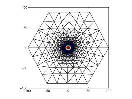
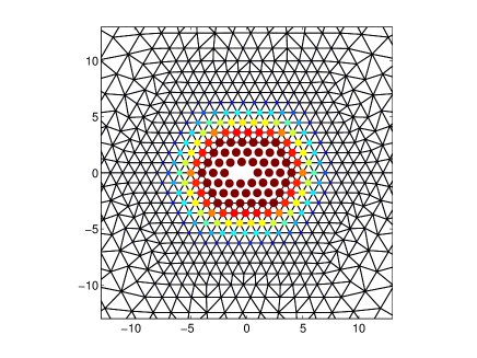
We choose the vacancy set $\mathcal{V}=\{0,e_{1}\}$ and the macroscopic strain

$$B=\left(\begin{matrix}1.03&0.3\\ 0.0&1.03\end{matrix}\right)\cdot B_{0},$$

where $B_{0}$ is a minimizer of $W$ ($3\%$ uniform stretch and $3\%$ shear from ground state). The setup of the B-QCF method for the di-vacancy problem is shown in Figure 10.

Figure 11. Plots of computational cost (DoF) versus error in the energy-norm for various a/c coupling methods approximating the di-vacancy problem described in section 4.3.1.

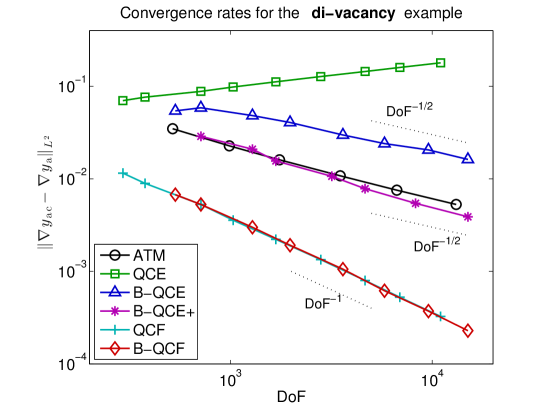
In Figure 11, we plot the degrees of freedom (DoF) against the error in the energy-norm for the various a/c coupling methods that we consider. As predicted by our analysis, the B-QCF method clearly outperforms all other methods, with the exception of the QCF method, which is barely distinguishable from the B-QCF method in this graph. Unfortunately, we cannot offer a satisfactory theory for the QCF method at present.

We also remark that, due to the high consistency error committed in the interface region, the B-QCE does not even outperform a plain atomistic computation in this particular example. (But it will clearly outperform the fully atomistic method (ATM) in the micro-crack example, where the elastic field is much more significant.)

4.3.2. The micro-crack example

Figure 12. Setup of the B-QCF method for the micro-crack example, for a specific choice of approximation parameters, shown in deformed equilibrium. The size/color of the atoms in the center correspond to decreasing values of $(1-\beta(x))$.

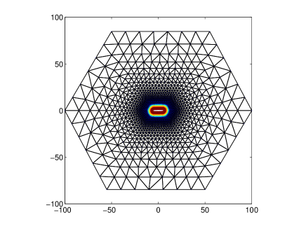
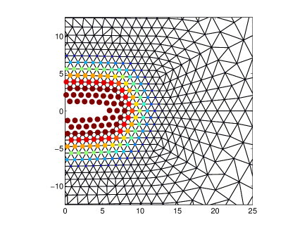
In the micro-crack (or void) example, we choose the vacancy set $\mathcal{V}=\{-5e_{1},\dots,5e_{1}\}$ and the macroscopic strain

$$B=\left(\begin{matrix}1.0&0.03\\ 0.0&1.03\end{matrix}\right)\cdot B_{0},$$

where $B_{0}$ is a minimizer of $W$ ($3\%$ tensile stretch and $3\%$ shear from ground state). The setup of the B-QCF method for the micro-crack problem is shown in Figure 12.

Figure 13. Plots of computational cost (DoF) versus error in the energy-norm for various a/c coupling methods approximating the micro-crack problem described in section 4.3.2.

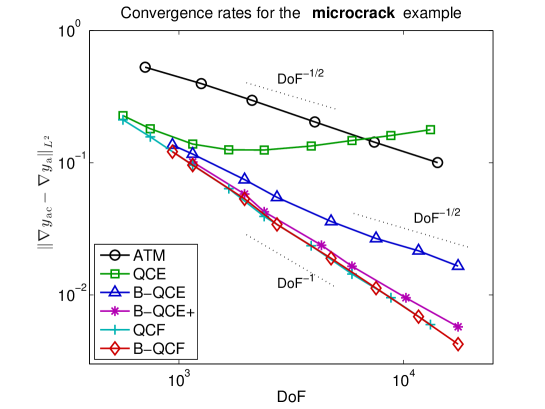
In Figure 13 we plot the degrees of freedom (DoF) against the error in the energy-norm, for the various a/c coupling methods that we consider. In this example the picture is less clear than in the di-vacancy example due to a more significant preasymptotic regime, which is caused by the more significant deformation admitted by the microcrack. In the preasymptotic regime we observe that the QCE and B-QCE methods perform much better than expected, but eventually fall back to the predicted rates. By contrast, the B-QCF and QCF methods display clear systematic convergence at the predicted rate throughout.

We also note that, in this example, the B-QCE+ method performs comparable to the B-QCF and QCF methods, at least in the preasymptotic regime accessible in the experiment.

5. Conclusion

We have formulated an atomistic-to-continuum force-based coupling, which we call the blended force-based quasicontinuum (B-QCF) method. In this paper, we numerically studied the stability as well as accuracy of the B-QCF method. We computed the critical strain errors between the atomistic and B-QCF models with different sizes of the blending region under different types of deformations.

The main theoretical conclusion in [21] is that the required blending width to ensure coercivity of the linearized B-QCF operator is surprisingly small. For both $1$D and $2$D uniform expansion, the computational results of the linearized operators perfectly match the analytic predictions. In addition, the stability for a general class of homogeneous deformations of the $2$D B-QCF operator becomes almost the same as that of the atomistic model by using a very small blending region, in contrast to the fact that the stability region of the force-based quasicontinuum (QCF) method, that is, the B-QCF method without blending region, is just a proper subset of the fully atomistic model. However, the critical strain error for the B-QCF operator applied to shear deformation seems to only linearly depend on the system size and is thus insensitive to blending width.

For the problem of a microcrack in a two-dimensional crystal, we studied the nonlinear stability of the B-QCF operators. The critical strain error decays faster than the prediction, and it can be as small as the strain increment. However, we find that the error increases a little bit when the blending size becomes larger, which is possibly due to round-off error.

Moreover, we implemented a practical version of the B-QCF method. We briefly reviewed the accuracy results in terms of computational cost [19]. The numerical experiments, di-vacancy and microcrack demonstrate the superior accuracy of B-QCF over other a/c coupling schemes that we have investigated previously in [27].

The BQCF method with a surprisingly small blending region is an appealing choice for numerical simulations of atomistic multi-scale problems as it is always consistent and can be guaranteed by both theory and benchmark testing to be positive definite when the fully atomistic operator is positive definite.

6. Acknowledgments

We appreciate helpful discussions with Brian Van Koten.

References

- [1] S. Badia, P. Bochev, R. Lehoucq, M. L. Parks, J. Fish, M. Nuggehally, and M. Gunzburger. A force-based blending model for atomistic-to-continuum coupling. International Journal for Multiscale Computational Engineering, 5:387–406, 2007.
- [2] S. Badia, M. Parks, P. Bochev, M. Gunzburger, and R. Lehoucq. On atomistic-to-continuum coupling by blending. Multiscale Model. Simul., 7(1):381–406, 2008.
- [3] P. T. Bauman, H. B. Dhia, N. Elkhodja, J. T. Oden, and S. Prudhomme. On the application of the Arlequin method to the coupling of particle and continuum models. Comput. Mech., 42(4):511–530, 2008.
- [4] T. Belytschko and S. P. Xiao. Coupling methods for continuum model with molecular model. International Journal for Multiscale Computational Engineering, 1:115–126, 2003.
- [5] T. Belytschko, S. P. Xiao, G. C. Schatz, and R. S. Ruoff. Atomistic simulations of nanotube fracture. Phys. Rev B, 65, 2002.
- [6] X. Blanc, C. Le Bris, and F. Legoll. Analysis of a prototypical multiscale method coupling atomistic and continuum mechanics. M2AN Math. Model. Numer. Anal., 39(4):797–826, 2005.
- [7] W. Curtin and R. Miller. Atomistic/continuum coupling in computational materials science. Modell. Simul. Mater. Sci. Eng., 11(3):R33–R68, 2003.
- [8] M. Dobson and M. Luskin. Analysis of a force-based quasicontinuum approximation. M2AN Math. Model. Numer. Anal., 42(1):113–139, 2008.
- [9] M. Dobson and M. Luskin. An analysis of the effect of ghost force oscillation on the quasicontinuum error. Mathematical Modelling and Numerical Analysis, 43:591–604, 2009.
- [10] M. Dobson, M. Luskin, and C. Ortner. Accuracy of quasicontinuum approximations near instabilities. Journal of the Mechanics and Physics of Solids, 58:1741–1757, 2010.
- [11] M. Dobson, M. Luskin, and C. Ortner. Sharp stability estimates for force-based quasicontinuum methods. SIAM J. Multiscale Modeling and Simulation, 8:782–802, 2010.
- [12] M. Dobson, M. Luskin, and C. Ortner. Stability, instability and error of the force-based quasicontinuum approximation. Archive for Rational Mechanics and Analysis, 197:179–202, 2010.
- [13] M. Dobson, M. Luskin, and C. Ortner. Iterative methods for the force-based quasicontinuum approximation. Computer Methods in Applied Mechanics and Engineering, 200:2697–2709, 2011.
- [14] M. Dobson, C. Ortner, and A. V. Shapeev. The Spectrum of the Force-Based Quasicontinuum Operator for a Homogeneous Periodic Chain. Multiscale Model. Simul., 10(3):744–765, 2012.
- [15] W. E, J. Lu, and J. Yang. Uniform accuracy of the quasicontinuum method. Phys. Rev. B, 74(21):214115, 2006.
- [16] J. Fish, M. A. Nuggehally, M. S. Shephard, C. R. Picu, S. Badia, M. L. Parks, and M. Gunzburger. Concurrent AtC coupling based on a blend of the continuum stress and the atomistic force. Comput. Methods Appl. Mech. Engrg., 196(45-48):4548–4560, 2007.
- [17] T. Hudson and C. Ortner. On the stability of Bravais lattices and their Cauchy–Born approximations. M2AN Math. Model. Numer. Anal., 46:81–110, 2012.
- [18] B. V. Koten and M. Luskin. Analysis of energy-based blended quasicontinuum approximations. SIAM. J. Numer. Anal., 49:2182–2209, 2011.
- [19] H. Li, M. Luskin, C. Ortner, A. V. Shapeev, and B. Van Koten. Blended atomistic/continuum hybrid methods. manuscript.
- [20] X. H. Li and M. Luskin. A generalized quasi-nonlocal atomistic-to-continuum coupling method with finite range interaction. IMA Journal of Numerical Analysis, 32:373–393, 2012.
- [21] X. H. Li, M. Luskin, and C. Ortner. Positive-definiteness of the blended force-based quasicontinuum method. SIAM J. Multiscale Modeling & Simulation, 10:1023– 1045, 2012. arXiv:1112.2528v1.
- [22] P. Lin. Convergence analysis of a quasi-continuum approximation for a two-dimensional material without defects. SIAM J. Numer. Anal., 45(1):313–332 (electronic), 2007.
- [23] W. K. Liu, H. Park, D. Qian, E. G. Karpov, H. Kadowaki, and G. J. Wagner. Bridging scale methods for nanomechanics and materials. Comput. Methods Appl. Mech. Engrg., 195:1407 –1421, 2006.
- [24] J. Lu and P. Ming. Stability of a force-based hybrid method in three dimension with sharp interface. ArXiv e-prints, Dec. 2012.
- [25] J. Lu and P. Ming. Convergence of a force-based hybrid method in three dimensions. Communications on Pure and Applied Mathematics, 66(1):83–108, 2013.
- [26] M. Luskin and C. Ortner. Atomistic-to-continuum coupling. Acta Numerica, 22:397–508, 4 2013.
- [27] M. Luskin, C. Ortner, and B. Van Koten. Formulation and optimization of the energy-based blended quasicontinuum method. Computer Methods in Applied Mechanics and Engineering, 253:160–168, 2013. arXiv: 1112.2377.
- [28] MATLAB. version 8 (R2012b). The MathWorks Inc., Natick, Massachusetts, 2010.
- [29] R. Miller and E. Tadmor. The quasicontinuum method: overview, applications and current directions. Journal of Computer-Aided Materials Design, 9:203–239, 2003.
- [30] R. Miller and E. Tadmor. Benchmarking multiscale methods. Modelling and Simulation in Materials Science and Engineering, 17:053001 (51pp), 2009.
- [31] P. Ming and J. Z. Yang. Analysis of a one-dimensional nonlocal quasi-continuum method. Multiscale Model. Simul., 7(4):1838–1875, 2009.
- [32] C. Ortner. A priori and a posteriori analysis of the quasinonlocal quasicontinuum method in 1D. Math. Comp., 80(275):1265–1285, 2011.
- [33] C. Ortner and A. V. Shapeev. Analysis of an energy-based atomistic/continuum approximation of a vacancy in the 2D triangular lattice. Math. Comp., 82:2191–2236, 2013. arXiv:1104.0311.
- [34] C. Ortner and L. Zhang. Construction and sharp consistency estimates for atomistic/continuum coupling methods with general interfaces: a 2D model problem. SIAM J. Numer. Anal., 50, 2012.
- [35] S. Prudhomme, H. Ben Dhia, P. T. Bauman, N. Elkhodja, and J. T. Oden. Computational analysis of modeling error for the coupling of particle and continuum models by the Arlequin method. Comput. Methods Appl. Mech. Engrg., 197(41-42):3399–3409, 2008.
- [36] P. Seleson and M. Gunzburger. Bridging methods for atomistic-to-continuum coupling and their implementation. Communications in Computational Physics, 7:831–876, 2010.
- [37] A. V. Shapeev. Consistent Energy-Based Atomistic/Continuum Coupling for Two-Body Potentials in One and Two Dimensions . SIAM Journal on Multiscale Modeling and Simulation, 9:905–932, 2011.
- [38] A. V. Shapeev. Consistent energy-based atomistic/continuum coupling for two-body potentials in three dimensions. SIAM Journal on Scientific Computing, 34(3):B335–B360, 2012.
- [39] V. B. Shenoy, R. Miller, E. B. Tadmor, D. Rodney, R. Phillips, and M. Ortiz. An adaptive finite element approach to atomic-scale mechanics–the quasicontinuum method. J. Mech. Phys. Solids, 47(3):611–642, 1999.
- [40] T. Shimokawa, J. Mortensen, J. Schiotz, and K. Jacobsen. Matching conditions in the quasicontinuum method: Removal of the error introduced at the interface between the coarse-grained and fully atomistic region. Phys. Rev. B, 69(21):214104, 2004.
- [41] E. B. Tadmor, M. Ortiz, and R. Phillips. Quasicontinuum analysis of defects in solids. Philosophical Magazine A, 73(6):1529–1563, 1996.
- [42] S. P. Xiao and T. Belytschko. A bridging domain method for coupling continua with molecular dynamics. Comput. Methods Appl. Mech. Engrg., 193(17-20):1645–1669, 2004.