The Effects of Inhomogeneities within Colliding Flows on the Formation and Evolution of Molecular Clouds

Abstract

Observational evidence from local star-forming regions mandates that star formation occurs shortly after, or even during, molecular cloud formation. Models of the formation of molecular clouds in large-scale converging flows have identified the physical mechanisms driving the necessary rapid fragmentation. They also point to global gravitational collapse driving supersonic turbulence in molecular clouds. Previous cloud formation models have focused on turbulence generation, gravitational collapse, magnetic fields, and feedback. Here, we explore the effect of structure in the flow on the resulting clouds and the ensuing gravitational collapse. We compare two extreme cases, one with a collision between two smooth streams, and one with streams containing small clumps. We find that structured converging flows lead to a delay of local gravitational collapse (“star formation”). Thus, more gas has time to accumulate, eventually leading to a strong global collapse, and thus to a high star formation rate. Uniform converging flows fragment hydrodynamically early on, leading to the rapid onset of local gravitational collapse and an overall low sink formation rate.

1 Introduction

The concept of flow-driven cloud formation (Vázquez-Semadeni et al., 1995; Ballesteros-Paredes et al., 1999; Hartmann et al., 2001) can explain two observational constraints on how molecular clouds form stars, derived from local star-forming regions: first, all local molecular clouds are observed to be forming stars, and second, the stellar age spreads are on the order of $1-2$ Myr, several times shorter than cloud crossing times (Hartmann et al., 2001; Ballesteros-Paredes & Hartmann, 2007, see summary in ). The first constraint suggests that star formation sets in immediately (or even during) molecular cloud formation, and that the second constraint is trivially fulfilled in a scenario where the clouds themselves form in large-scale “converging” flows. The immediate (“rapid”) onset of star formation in the forming clouds and the fact that the star formation efficiency is only a few percent (Evans et al., 2009) mandates that the clouds are highly structured: local collapse must set in before global collapse can overwhelm the dynamics.

The notion of cloud formation in converging flows has led to a series of numerical experiments investigating the physical processes relevant for the rapid fragmentation and for the control of the star formation efficiency. There is agreement across the models (despite different initial and boundary conditions) on the following results: (1) Rapid fragmentation is induced by strong radiative losses during the flow collision (possibly even by thermal instability if the clouds form from atomic gas), and by dynamical instabilities (Hueckstaedt, 2003; Audit & Hennebelle, 2005; Vázquez-Semadeni et al., 2006; Heitsch et al., 2008b) (2) Turbulence in molecular clouds is a natural result of the dynamical instabilities during the cloud formation, and is driven by global gravitational collapse at later stages of the cloud evolution (Vázquez-Semadeni et al., 2007). (3) Strong, non-linear density contrasts can also be driven by self-gravity in finite clouds, due to geometry (or “edge”) effects (Burkert & Hartmann, 2004). (4) Although the rapid fragmentation can keep the star formation efficiency low, eventually, feedback or cloud dispersal is needed to prevent a large percentage of the gas to participate in gravitational collapse (Vázquez-Semadeni et al., 2010).

The most obvious difference in the simulation results is the morphology of the forming clouds. All models use some mechanism to break the symmetry in the colliding flows – otherwise, the flow collision would result in a plane-parallel shock. Models with small-scale perturbations (“noise”) in the velocities tend to lead to extremely flattened clouds with a strong ring due to the gravitational edge effect (Burkert & Hartmann, 2004; Hartmann & Burkert, 2007) in finite, sheet-like clouds. If the velocity perturbations are imposed on larger scales (e.g as a turbulent power spectrum), or if the collision interface between the two flows is perturbed, turbulent structures form that are not necessarily coherent when viewed from different directions (Heitsch et al., 2009).

To understand better the effect of initial conditions on the clouds forming in the flow collisions, we present a simple experiment, comparing two (otherwise identical) cloud formation simulations, one with a smooth inflow, and one with a clumpy inflow of identical mass. The experiment is also motivated by the analysis of Pringle et al. (2001), suggesting that cloud formation out of warm atomic gas would require time and length scales too large to be feasible (see also McKee & Ostriker (2007)). This problem is solved by the realization that the flow collision is three-dimensional, allowing gravitational collapse and accretion along the dimensions perpendicular to the flows, and thus circumventing the one-dimensional limit on column density accumulation (Heitsch et al., 2008a). Yet, Pringle et al. (2001) suggest that clumpy flows could reduce the accumulation and molecule formation time scale (especially if the clumps are already molecular). Here, we will test, what effects a clumpy flow has on the resulting cloud and star formation process.

2 Method, Initial Conditions, and Parameters

To model a finite molecular cloud forming in a collision of two flows, we use the adaptive-mesh-refinement code AstroBEAR 2.0 to solve the equations of hydrodynamics including self-gravity and equilibrium cooling. For a detailed discussion of AstroBEAR, see Carroll-Nellenback et al. (2013). Poisson’s equation is solved with HYPRE (Falgout & Yang, 2002). We used a non-split CTU integrator following Gardiner & Stone (2008), and the sink particle implementation discussed by Federrath et al. (2010).

We performed two simulations of $40$ pc diameter flows with a mean density $n=1.0$ cm^-3, colliding head-on at $v_{0}=8.25$ km s^-1 for a period of 30 Myr. The flows collide in the y-z plane within a box that is $62.5\times 100\times 100$ pc³ in size. We use a base grid of $40\times 64\times 64$ cells with $5$ additional levels of refinement for an effective resolution of $1280\times 2048\times 2048$ and a physical cell size of $\approx 0.05$ pc. The flows combine to give a mass flux of $\dot{M}=665$ M_☉ Myr^-1 and a ram pressure of $P_{\mbox{ram}}=10472$ K cm^-3. We used an ideal equation of state at $\gamma=5/3$, with a mean particle mass $\chi=1.27$ and a parametrized cooling function $\mathcal{S}$ that includes heating terms consistent with Inoue & Inutsuka (2008) though modified to give lower temperatures $10$ K at higher densities ($n>10^{3}$ cm^-3) to account for UV shielding (Ryan & Heitsch in prep).

$$\begin{array}[]{l}\mathcal{S}=n(-\Gamma+n\Lambda)\mbox{erg cm}^{-3}\mbox{s}^{-1}\\ \Gamma=2\times 10^{-26}\\ \frac{\Lambda}{\Gamma}=1.0\times 10^{7}\exp{\left(\frac{-118400}{T+1000}\right)}+1.4\times 10^{-2}\sqrt{T}\exp{\left(\frac{-22.75}{\max{\left[1.0,T-4\right]}}\right)}\end{array}$$ (1)

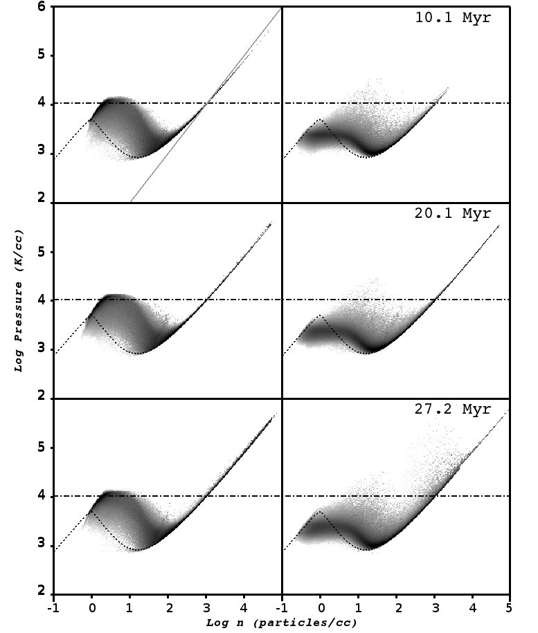
The combined heating and cooling results in a thermal equilibrium pressure for each density. This curve can be seen in the dashed line of figure 1. Note the dashed line only extends to densities of $10^{2}$ cm^-3 to avoid confusion at higher densities - but the equilibrium curve can be seen at higher densities in the distribution itself because the thermal timescales are much smaller than any other time scale at those densities, and thus the gas lines up with the equilibrium curve. In the “Smooth” simulation, the inflowing gas has a uniform density of $1.0$ cm^-3 and a thermal equilibrium pressure of $4931$ K cm^-3. For the “Clumpy” simulation, the mean inflow density is also $1.0$ cm^-3, yet the flow contains many small clumps of radius $0.55$ pc and a density of $15.2$ cm^-3, placed randomly in a smooth lower background density of $0.25$ cm^-3. Both the clumps and the low density background are in pressure equilibrium at $6857$ K cm^-3 and both are stable to thermal instabilities, though they are not in thermal equilibrium with each other. The high density contrast $\chi=60.8$ between clumps and background results in a filling fraction of $f=0.05$. The clump radius was chosen to be much less than the Jeans length at the clump density and pressure ($L_{J}=43.3$ pc) so that the clumps would be stable against gravitational collapse. In both runs, the interface between oppositely directed material is initially rippled with a random sequence of sines and cosines of amplitude $2$ pc, wavelengths from 40 pc down to $2.5$ pc and power proportional to $k^{-3}$.

Figure 1: Density-weighted joint probability distribution function for density vs. pressure for the Smooth run (left) and Clumpy run (right), at $10.1,20.1$, and $27.2$ Myr. The dot-dashed line indicates the ram pressure of the flows, and the diagonal line in the upper left plot shows $T\equiv 10$ K.

3 Results

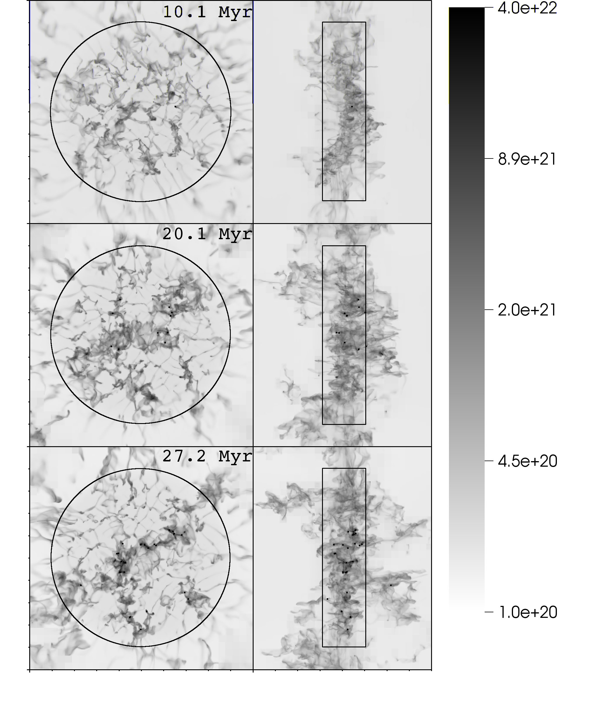
All of the following analysis focuses on a hockey-puck shaped region that is $40$ pc in diameter and $10$ pc thick, centered on the interface between the two flows. This region is outlined in figures 2 and 3. Figure 1 shows the joint probability distribution in logarithmic density-pressure space for both runs at times $10.1,20.1$, and $27.2$ Myr.

3.1 Thermal Properties

In the Smooth model (left column), material enters the collision region on the equilibrium curve at $1.0$ cm^-3 which coincides with the peak in the equilibrium cooling curve. As the material collides with the oppositely directed material it is initially compressed adiabatically up to the flow ram pressure at $1.04\times 10^{4}$ cm^-3. It then cools and compresses onto the thermal equilibrium curve. With time, more material piles up at higher densities. Eventually, self-gravity takes over at the highest densities and compresses this material further, above the ram pressure provided by the flow. At this point, gas collapses and forms a core, or is being accreted by an existing core. The core formation or accretion explains the lack of material at densities above $\approx 10^{4.6}$ cm^-3.

The Clumpy flow on the other hand (right column) has material entering the collision region at both $0.25$ cm^-3 and $15.2$ cm^-3. Additionally, some mixing occurs between the clumps and the background flow which causes the thick band of material below the thermal equilibrium curve. At these densities, the thermal time scales are longer than the dynamical time [see Fig. 3 of Heitsch et al. (2008b)] - so this material does not equilibrate before colliding with the oppositely directed flow. The low density background appears to also compress adiabatically though not to as high pressures as the Smooth run. At the interface between the two flows there are three possible types of interactions due to the two densities present in the flow: (a) For background-background collisions, the ram pressure will be $1/4$th of that for the Smooth flow. (b) Collisions between background material from one side and clumps from the other will produce bow shocks equivalent to background material running over a stationary clump with velocity $2v_{0}=16.5$ km s^-1, resulting in a ram pressure equal to that in the Smooth model, at $1.04\times 10^{4}$ K cm^-3. (c) Finally, head-on clump-clump collisions, though rare, can produce pressures $15.2$ times the ram pressure in the Smooth model. Yet this material will cool fairly quickly due to the high densities.

3.2 Morphologies

Figures 2 and 3 show column densities taken along the flow axis (left) and normal to the flow axis (right) for the Smooth and Clumpy runs respectively. Also shown are the boundaries of the “hockey puck” region used for the following analysis. The Smooth run exhibits the usual filamentary structure due primarily to the non-linear thin shell instability [NTSI, (Vishniac, 1994; Hueckstaedt, 2003; Heitsch et al., 2005; Vázquez-Semadeni et al., 2006)], and at later times gravity. Also visible is material which has been “splashed” radially outward from the collision region due to the high ram pressures. The NTSI focuses material into various nodes and by $10.1$ Myr the first core (solid black square) has formed in one of these nodes (Heitsch et al., 2008a, see also). By $20.1$ Myr, nine cores have formed throughout the complex and by $27.2$ Myr, $27$ cores have begun to arrange themselves into clusters.

Figure 2: Column density in units of cm^-2 projected parallel (left) and perpendicular (right) to flow axis, at $10.1,20.1$, and $27.2$ Myr for the Smooth run. Sink particles appear as small black squares. Tick-marks are spaced every 5 pc and each panel is $50$ pc tall.

Figure 3: Column density in units of cm^-2, projected parallel (left) and perpendicular (right) to flow axis, at $10.1,20.1$, and $27.2$ Myr for the Clumpy run. Sink particles appear as small black squares.

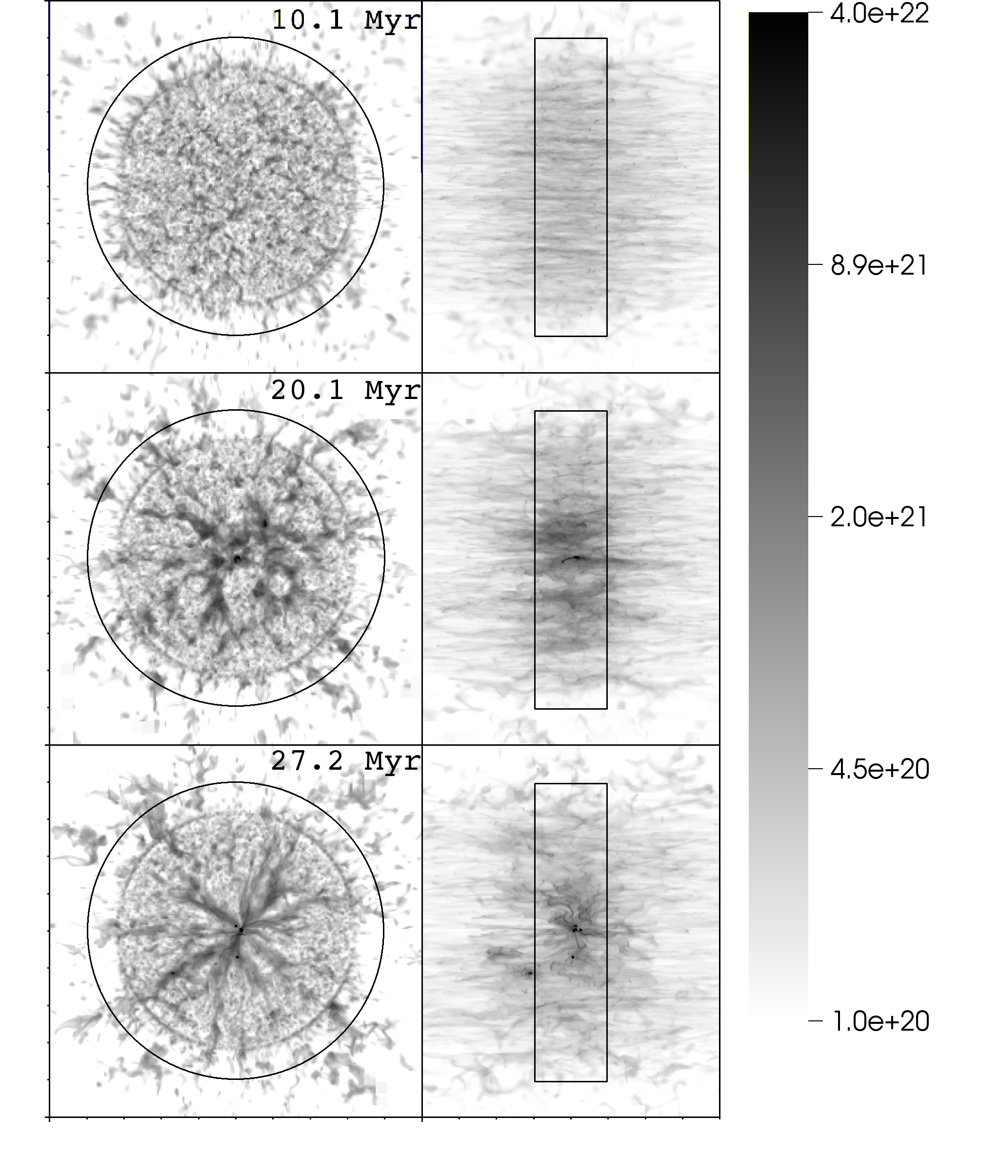
The morphology of the Clumpy run (Figure 3) is quite different from the Smooth run. The view along the flow axis shows that the clumps are confined to be within the stream by a few pc and they have a tendency to cluster around the perimeter. This is just an artifact of the clump placing algorithm and can be safely ignored. There also tends to be much less radial splashing than in the Smooth run because the uniform background component prone to being splashed out is only $1/4$th as dense. The interaction region is much more extended along the flow axis than in the Smooth run. Early on, dense clumps run into the lighter background and travel a distance before being destroyed. The timescale for the clump destruction will be of order the clump crushing time $t_{cc}=\frac{\chi r_{c}}{v_{w}}$ (Klein et al., 1994) where $v_{w}$ is the ‘wind velocity’ as seen by the clump and $\chi$ is the density contrast. Since the clump is itself traveling into an oppositely directed flow, $v_{w}=2v_{0}$ and the distance the clump will travel will be of order

$$\mathcal{D}=t_{cc}v_{0}=\frac{\chi r_{c}}{2}=4.3\mbox{ pc}.$$ (2)

If the clump survives for a few clump crushing times, it will travel distances of $\approx 10$ pc before being destroyed. This explains the more extended interaction region in the upper right panel of figure 3. Later in time, the clumps pass through a denser wall of material that has built up and they are also pulled back by gravity - so the extent of the collision region shrinks over time. While the Smooth run has formed nine isolated cores by $20.1$ Myr distributed throughout the collision region, the Clumpy run has only just formed a group of three cores near the center of the global potential well. By $27.$ Myr, the entire region is undergoing rapid global collapse and a dense group of $20$ cores has formed again near the center of the potential well.

3.3 Spectra

To generate spectra we first take a cube of size $d=40.625$ pc, centered on the simulation domain. The data within the cube is then windowed with

$$w(r)=\left\{\begin{array}[]{ll}\cos(\pi r/d)&:r<=d/2\\ 0&:r>d/2\end{array}\right.$$

The process of mapping AMR data onto a fixed grid often leads to spurious signals at wavelengths corresponding to coarser cell sizes. To reduce this effect we prolongated in Fourier space instead of physical space. The coarse data within the cube was transformed into Fourier space, and the various components were then mapped onto a finer Fourier grid. A phase was then added to each Fourier component (since finer cells are not collocated with their coarser parent cells) before being transformed back into physical space. Then this prolongated grid was updated with existing data on the next finest level and the process was repeated.

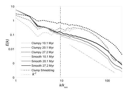
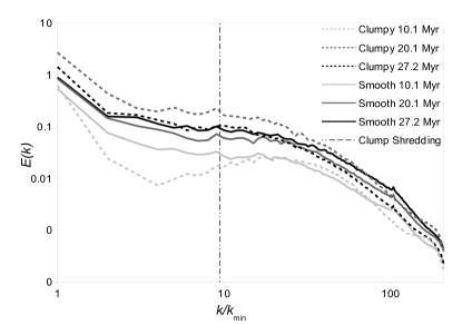
Figure 4 shows the kinetic and gravitational energy spectra. At $10.1$ Myr, the Clumpy run has an excess of kinetic energy at small scales and a lack of kinetic energy at large scales. While both runs have the same flux of kinetic energy, the Clumpy run contains most of the kinetic energy in dense clumps on small scales. When these flows collide, the clumps are able to maintain coherence until they have travelled a clump shredding distance (eq. 2) at which point their kinetic energy is able to dissipate. This clump shredding distance can be thought of as a ‘driving scale’ for the small scale ‘turbulence’ and roughly corresponds to the break in the power spectrum.

By $20.1$ Myr, the Clumpy run has gained large scale energy due to the onset of global collapse, and by $27.2$ Myr the Clumpy run has gained energy on all scales due to both the continued global collapse as well as the onset of local collapse. The Smooth run on the other hand does not show any growth of large scale kinetic energy, with modest growth of smaller scale kinetic energy. This picture is confirmed by the gravitational energy spectra - thought it should be mentioned that both spectra are for non-accreted gas. The overall drop in gravitational energy in the Clumpy run between 20.1 and 27.2 Myr is due to the very rapid accretion onto sink particles, following the global collapse.

Figure 4: Kinetic energy (left) and gravitational energy spectra (right) for both runs and three times as indicated in the diagram. The vertical line indicates the clump shredding distance (eq. 2).

3.4 Energy budgets

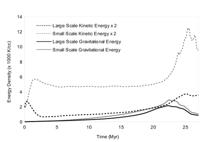
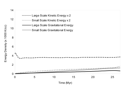
Figure 5 shows the evolution the energy densities at large and small scales. We choose the clump shredding distance $\mathcal{D}=4.3$ pc (see eq. 2) as the dividing line between “small” and “large” scales. For the Smooth run (right panel) we note that the kinetic energy on large scales is always greater than the large scale gravitational energy. This is consistent with the lack of global collapse observed for the Smooth run. However, the small scale gravitational energy becomes comparable to the small scale kinetic energy after $10$ Myr which is when we begin to see the formation of isolated cores, indicating local collapse. The Clumpy run on the other hand shows the opposite – the energy is dominated by small scale kinetic energy which suppresses local collapse. Only after $20$ Myr, when the large scale gravitational energy becomes comparable to the large scale kinetic energy, do we begin to see global collapse. By $23$ Myr, much of the gas has been accreted into several large cores near the center of the potential well, which explains the drop in energies.

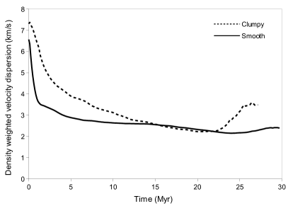
While both runs begin with the same total kinetic energy, and while they have the same flux of kinetic energy, the Smooth run is much more efficient at dissipating this energy in large coherent shocks resulting in a smaller overall kinetic energy within the collision zone. In the Clumpy run, the density contrast between the clumps and the opposing ambient material leads to a less efficient dissipation of kinetic energy. This excess kinetic energy on small scales suppresses local collapse (remember that the clumps themselves are gravitationally stable) but cannot prevent global collapse - while in the Smooth run, the higher degree of kinetic energy on large scales resists global collapse but not local collapse. Another way to see this is that the shocks in the Smooth run will fragment quickly due to the thermal instability. Yet, the velocity dispersion between the fragments will be small, at least smaller than for the Clumpy run (see Fig. 6, right), thus forming structures that are more or less coherent in velocity space. Thus, local collapse is seeded. For the Clumpy run, thermal instability does not play much of a role, and gas accretion onto the clumps due to cooling or gravity is negligible within the (dynamical) timescales considered. Thus, local collapse is suppressed, while global collapse sets in once enough mass in clumps has been assembled.

Figure 5: Plots showing time evolution of mean kinetic and gravitational energy densities split between large ($>\mathcal{D}$, see eq. 2) and small scales for both the Clumpy run (left) and the Smooth run (right).

3.5 Core Formation

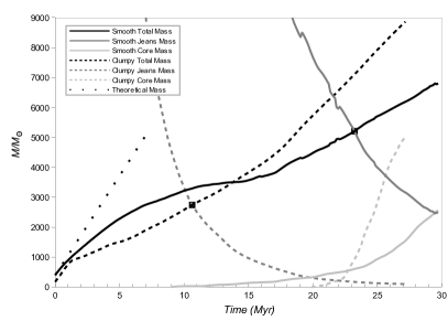
The left panel of Figure 6 shows the growth in total mass within the collision region as well as the theoretical upper bound (dotted line) using the mass flux $\dot{M}$. Both runs collect mass at the inflow rate $\dot{M}$ for the first two Myr, after which the growth rate drops. For the Smooth run, material is being splashed radially outwards, and at later times, some of the NTSI fingers develop past the analysis region (see Fig. 2). Eventually, after $15$ Myr, material is falling back in from the edges of the analysis region, increasing the mass collection rate again. In the Clumpy run, some of the clumps exit the analysis region on the far side after $2$ Myr. The overall mass collection rate slowly increases after that, with material falling back in, and eventually collapsing globally.

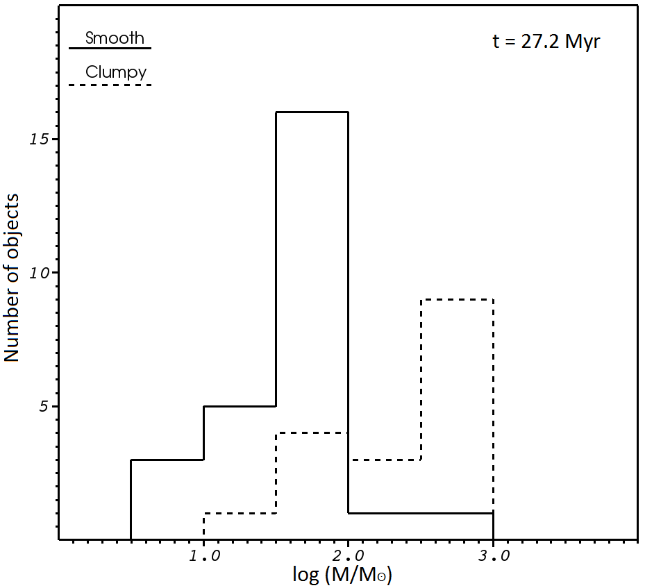
The Smooth run begins forming cores at $10$ Myr, and by $25$ Myr, the rate of total mass growth and core mass growth have become equal. This implies that material is being accreted by the cores at the same rate it is entering the collision region. The Clumpy run (Figure 3) does not begin to form cores until $20$ Myr, but then quickly accretes gas at a rate higher than the mass flux into the region. This suggests a degree of global collapse not present in the Smooth run.

Since the gas is being compressed and cooled, the Jeans mass at a given sound speed $c_{s}$ and a mass column density $\Sigma$

$$M_{J}=1.17\frac{c_{s}^{4}}{G^{2}\Sigma}$$ (3)

will drop with time, as shown in Figure 6 (left panel). It levels out once the minimum temperature of $\approx 10$ K is reached (this is only obvious in the Clumpy run, dashed lines, for $t>25$ Myr. The Jeans mass for the Clumpy run is smaller by at least an order of magnitude, because of the clumps at higher densities and lower temperatures. Yet, since these clumps do not form a coherent region with $M>M_{J}$, local gravitational collapse is suppressed until $\approx 20$ Myr, and sinks form only once global collapse sets in, indicated by the increasing slope of the total mass, black dashed line. The onset of global collapse in the Clumpy run is also visible in Figure 5 (left), and in the velocity dispersions shown in the right panel of Figure 6.

The Smooth run has a substantially larger Jeans mass that does not level out at a minimum within the model run time. Yet, because of the rapid local fragmentation into structures larger than a local Jeans mass, local collapse (and sink formation) sets in at $\approx 10$ Myr. There is no signature of global collapse in the velocity dispersions, or in the energies.

Figure 6: Left: Mass history against time for the Clumpy and Smooth run. Black lines indicate total mass in the analysis region, dark gray lines trace the Jeans mass, also in the analysis region, and the light gray lines follow the mass in sinks, tracing local collapse. The dotted line stands for the mass accumulation expected from simple sweep-up. Local collapse is suppressed in the Clumpy run until $\approx 20$ Myr, while the Smooth run forms sinks after $\approx 10$ Myr. Right: Density-weighted velocity dispersion against time, for the Clumpy and Smooth run, again within the analysis region. The Clumpy dispersion is systematically higher until $\approx 15$ Myr, and increases again once global collapse sets in at $22$ Myr.

Figure 7: Core mass distribution at $27.2$ Myr. Cores in the Smooth run tend to have less mass than those in the Clumpy run.

Figure 7 shows the distribution of core masses for both runs at $27.2$ Myr. The Smooth run forms many intermediate sized cores $<100$ M_☉ consistent with the idea of local collapse. The Clumpy run shows many more high density cores ($100-1000$ M_☉) visible in the center of the potential well (Fig. 3) due to global collapse.

3.6 Mixing

In both runs, material injected from the left and right side was marked with a tracer ($\rho_{L}$ and $\rho_{R}$) proportional to the density so that the amount of mixing could be investigated. We then define a mixing ratio

$$MR=\frac{2\min{\left(\rho_{L},\rho_{R}\right)}}{\max{\left(\rho,\rho_{L}+\rho_{R}\right)}}.$$ (4)

Thus, $MR=0$ indicates the presence of only one tracer (or none - as is the case in the ambient medium outside of the flow), and $MR=1$ indicates equal amounts of both tracers with no ambient material mixed in. Since we are confining our analysis to the colliding flow region, there should be no ambient material present so $\rho=\rho_{L}+\rho_{R}$ - and the definition is equivalent to

$$MR=\frac{2\min{\left(\rho_{L},\rho_{R}\right)}}{\rho_{L}+\rho_{R}}.$$ (5)

Figure 8: Left: Mass-weighted mixing ratio (eq. 5) for the gas in the analysis region, at $10.1$ Myr. Right: Mixing ratio of cores at $27.2$ Myr.

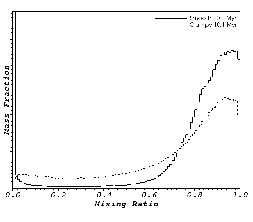
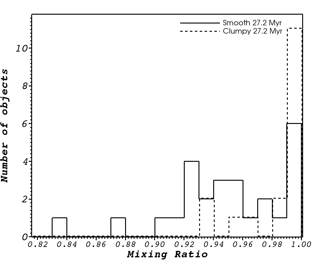
In the Smooth run, there is a higher mass-fraction of well-mixed material (Fig. 8, left panel; note that the total masses in the analysis region at that time are comparable). The Clumpy run tends to have a more spread out distribution of mixing ratios than the Smooth run. As clumps drive through the opposing stream - they will shed some of their material and provide varying amounts of mixing. In the Smooth case, the flows interact along a thin interface and it is difficult to get unequal amounts of material from either side in the same region. One might expect the Clumpy run to have less well-mixed cores, yet the right panel of figure 8 shows just the opposite. The Smooth run has more cores with lower mixing ratios.

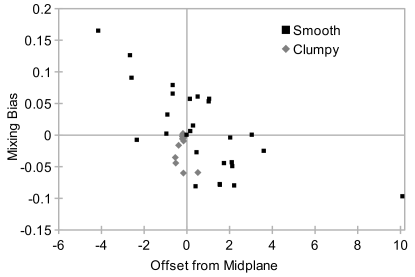
One possible explanation for this is that the NTSI creates nodes that act to funnel material streaming into the “trough” from only side, while diverting material from the other side. If so, then cores that formed to the left of the collisional mid-plane should be biased towards the right tracer and vice versa. To test this, we define a mixing bias as

$$MB=\frac{\rho_{R}-\rho_{L}}{\rho_{R}+\rho_{L}}$$ (6)

and plot it against the core’s distance from the y-z mid-plane (Fig. 9). Indeed, cores with negative offsets (left of mid-plane) tend to have a higher value for the mixing bias so they have more right tracer and are comprised of material primarily from the right side, and vice versa. Note that this bias is absent in the cores formed in the Clumpy run, whose cores are clustered around $0$.

Figure 9: Mixing Bias (eq. 6) against distance of cores to mid-plane, at $27.2$ Myr. Smooth cores show a bias, while Clumpy cores are clustered around $0$.

4 Discussion and Conclusion

We present the results of two simulations of flow-driven molecular cloud formation. The models are identical except for the physical conditions of the inflowing gas. One model (“Smooth”) starts out with a completely uniform flow. The other model (“Clumpy”) uses the same mass inflow rate, but the gas is distributed in dense clumplets with a filling factor of $5$%. This setup is in parts motivated by Pringle’s et al. 2001 claim that in order to form molecular clouds from atomic gas sufficiently fast, dense pockets of already molecular gas should exist in the inflow. Here, we are focusing on the resulting dynamics of smooth versus clumpy inflows.

In both cases, the thermal and dynamical fragmentation of the shocked collision region leads to turbulence, at a level of $10$ to $20$% of the inflowing kinetic energy. This is consistent with earlier results. The Clumpy run shows a somewhat higher velocity dispersion initially, since the clumps are less easily stopped in a flow collision (see §3.2).

Due to the lower compression factor in the Clumpy model, less gas is being cooled to higher densities than in the Smooth run. Thus, the kinetic energy of the inflow is less efficiently dissipated. Together with a non-contiguous distribution of cold, sub-jeans, fragments, this leads to a suppression of local collapse for nearly $20$ Myr after the initial flow collision. At that point, sufficient mass has assembled to induce global collapse of the whole region, resulting in a “star burst” (more appropriately, “sink burst”) at a high sink formation rate. In contrast, the Smooth run shows local collapse already after $10$ Myr, at less than half the sink formation rate of the Clumpy run. Due to the local nature of the thermal fragmentation, more fragmentation will occur with increasing resolution (Hennebelle & Audit, 2007), thus, the times quoted here are upper limits for the onset of local collapse. Nevertheless, structured flows can delay the onset of (substantial) local collapse. Global collapse is only clearly visible in the Clumpy run.

The differences between Clumpy and Smooth inflows extend to the mixing efficiencies. Somewhat counter to a naive expectation, the Smooth initial conditions result in less well mixed material (and cores). This is primarily due to the NTSI funneling material preferentially into the troughs located far into the opposing inflow. For the Clumpy run, the global collapse of the accumulated clumps erases all memory of the initial inflow direction.

Obviously, we have chosen two extremes as our initial conditions. It is more likely that the inflows themselves will contain turbulent velocity and density structures that are coherent in space. Spatial coherence leads to stronger shocks in the collision region, and thus to more efficient energy dissipation. In that sense, our Clumpy run is overestimating the effect of structured inflows.

References

- Audit & Hennebelle (2005) Audit, E., & Hennebelle, P. 2005, A&A, 433, 1
- Ballesteros-Paredes et al. (1999) Ballesteros-Paredes, J., Hartmann, L., & Vázquez-Semadeni, E. 1999, ApJ, 527, 285
- Ballesteros-Paredes & Hartmann (2007) Ballesteros-Paredes, J., & Hartmann. L. 2007, Revista Mexicana de Astronomia y Astrofisica, 43, 123
- Burkert & Hartmann (2004) Burkert, A., & Hartmann, L. 2004, ApJ, 616, 288
- Carroll-Nellenback et al. (2013) Carroll-Nellenback, J. J., Shroyer, B., Frank, A., & Ding, C. 2013, Journal of Computational Physics, 236, 461
- Evans et al. (2009) Evans, II, N. J., Dunham, M. M., Jørgensen, J. K. et al. 2009, ApJS, 181, 321
- Falgout & Yang (2002) Falgout, R. & Yang, U. 2002, in Computational Science - ICCS 2002, ed. P. Sloot et al. (Springer Berlin Heidelberg), 632
- Federrath et al. (2010) Federrath, C., Banerjee, R., Clark, P. C., & Klessen, R. S. 2010, ApJ, 713, 269
- Gardiner & Stone (2008) Gardiner, T. A. & Stone, J. M. 2008, JCoPh 227, 4123
- Hartmann et al. (2001) Hartmann, L., Ballesteros-Paredes, J., & Bergin, E. A. 2001, ApJ, 562, 852
- Hartmann & Burkert (2007) Hartmann, L., & Burkert, A. 2007, ApJ, 654, 988
- Heitsch et al. (2005) Heitsch, F., Burkert, A., Hartmann, L. W., Slyz, A. D., & Devriendt, J. E. G. 2005, ApJ, 633, 113
- Heitsch et al. (2008a) Heitsch, F., Hartmann, L. W., Slyz, A. D., Devriendt, J. E. G., & Burkert, A. 2008, ApJ, 674, 316
- Heitsch et al. (2008b) Heitsch, F., Hartmann, L. W., & Burkert, A. 2008, ApJ, 683, 786
- Heitsch & Hartmann (2008) Heitsch, F., & Hartmann, L. 2008, ApJ, 689, 290
- Heitsch et al. (2009) Heitsch, F., Ballesteros-Paredes, J., & Hartmann, L. W. 2009, ApJ, 704, 1735
- Hennebelle & Audit (2007) Hennebelle, P., & Audit, E. 2007, A&A, 465, 431
- Hueckstaedt (2003) Hueckstaedt, R. M. 2003, New Astronomy, 8, 295
- Inoue & Inutsuka (2008) Inoue, T. & Inutsuka, S. 2008 arxiv, arxiv:0801.0486v2
- Klein et al. (1994) Klein, R. I., McKee, C. F., & Colella, P. 1994, ApJ420, 213
- McKee & Ostriker (2007) McKee, C. F., & Ostriker, E. C. 2007, ARA&A, 45, 565
- Pringle et al. (2001) Pringle, J. E., Allen, R. J., & Lubow, S. H. 2001, MNRAS, 327, 663
- Vázquez-Semadeni et al. (1995) Vázquez-Semadeni, E., Passot, T., & Pouquet, A. 1995, ApJ, 441, 702
- Vázquez-Semadeni et al. (2006) Vázquez-Semadeni, E., Ryu, D., Passot, T., González, R. F., & Gazol, A. 2006 ApJ643, 245
- Vázquez-Semadeni et al. (2007) Vázquez-Semadeni, E., Gómez, G. .C., Jappsen, A. K., Ballesteros-Paredes, J., González, R. F., & Klessen, R. S. 2007, ApJ, 657, 870
- Vázquez-Semadeni et al. (2010) Vázquez-Semadeni, E., Colín, P., Gómez, G. C., Ballesteros-Paredes, J., & Watson, A. W. 2010, ApJ, 715, 1302
- Vishniac (1994) Vishniac, E. T. 1994, ApJ, 428, 186