Remarks on the Cauchy problem for the one-dimensional quadratic (fractional) heat equation

Abstract.

We prove that the Cauchy problem associated with the one dimensional quadratic (fractional) heat equation: $u_{t}=D_{x}^{2\alpha}u\mp u^{2},\;t\in(0,T),\;x\in{\TenEns R}$ or ${\TenEns T}$, with $0<\alpha\leq 1$ is well-posed in $H^{s}$ for $s\geq\max(-\alpha,1/2-2\alpha)$ except in the case $\alpha=1/2$ where it is shown to be well-posed for $s>-1/2$ and ill-posed for $s=-1/2$. As a by-product we improve the known well-posedness results for the heat equation ($\alpha=1$) by reaching the end-point Sobolev index $s=-1$. Finally, in the case $1/2<\alpha\leq 1$, we also prove optimal results in the Besov spaces $B^{s,q}_{2}.$

Keywords: Nonlinear heat equation, Fractional heat equation, Ill-posedness, Well-posedness, Sobolev spaces, Besov spaces.

2000 AMS Classification: 35K15, 35K55, 35K65, 35B40

1. Introduction and main results

The Cauchy problem for the quadratic fractional heat equation reads

(1.1) $$u_{t}-D_{x}^{2\alpha}u=\mp u^{2},$$

(1.2) $$u(0,\cdot)=u_{0},$$

where $u=u(t,x)\in{\TenEns R}\;,\alpha\in]0,1],\;t\in(0,T),\;T>0,\;x\in{\TenEns R}$ or ${\TenEns T}$ and $D^{2\alpha}_{x}$ is the Fourier multiplier by $|\xi|^{2\alpha}$. In this paper, we consider actually the corresponding integral equation which is given by

(1.3) $$u(t)=S_{\alpha}(t)u_{0}\mp\int_{0}^{t}S_{\alpha}(t-\sigma)\big{(}u^{2}(\sigma)\big{)}d\sigma,$$

where $S_{\alpha}(t)$ is the linear fractional heat semi-group and are interested in local well-posedness and ill-posedness results in the Besov spaces $B^{s,q}_{2}(K)$ with $s\in{\TenEns R}$, $q\in[1,\infty[$ and $K={\TenEns R}$ or ${\TenEns T}.$

Let us recall that the Cauchy problem associated with the nonlinear heat equation in ${\TenEns R}^{n}$

(1.4) $$u_{t}-\Delta u=\mp u^{k}$$

has been studied in many papers (see for instance [3, 4, 5, 6, 7, 9, 11, 12, 13, 14, 18, 19, 20, 21] and references therein). It is well-known that this equation is invariant by the space-time dilation symmetry $u(t,x)\mapsto u_{\lambda}(t,x)=\lambda^{2\over k-1}u(\lambda^{2}t,\lambda x)$ and that the homogeneous Sobolev space $\dot{H}^{\frac{n}{2}-\frac{2}{k-1}}$ is invariant by the associated space dilation symmetry $\varphi(x)\mapsto\lambda^{2\over k-1}\varphi(\lambda x)$. The Cauchy problem (1.4) is known to be well-posed in $H^{s}$ for $s\geq s_{c}=\frac{n}{2}-\frac{2}{k-1}$ except in the case $(n,k)=(1,2)$. Indeed, in this case the well-posedness is only known in $H^{s}$ for $s>-1$ and in [9] it is proven that the flow-map cannot be of class $C^{2}$ below $H^{-1}$. Hence, this result is close to be optimal if one requires the smoothness of the flow-map. Recently, it was proven in [8] that the associated solution-map : $u_{0}\mapsto u$ cannot be even continuous in $H^{s}$ for $s<-1$. The first aim of this work is to push down the well-posedness result to the end point $H^{-1}$. The second step is to extend these type of results for the one-dimensional quadratic fractional heat equation (1.1). Indeed we will derive optimal results for the Cauchy problem (1.1) in the scale of the Besov spaces $B^{s,q}_{2}$ in the case $\frac{1}{2}<\alpha\leq 1$. In particular we will prove that the lowest reachable Sobolev index is $-\alpha$ that is strictly bigger then the critical Sobolev index for dilation symmetry that is $1/2-2\alpha$.
To reach the end-point index $H^{-\alpha}$ we do not follow the classical method for parabolic equations (cf. [4, 12, 21]) that does not seem to be applicable here. We rather rely on an approach that was first introduced by Tataru [16] in the context of wave maps. Note that we mainly follow [10] where this method has been adapted for dispersive-dissipative equations. The fact that our equation is purely parabolic enables us to simplify the proof. The optimality of our results follows from an approach first introduced by Bejenaru-Tao [1] for a one-dimensional quadratic Schrödinger equation. This approach is based on a high-to low frequency cascade argument.

Finally we consider the case $0<\alpha\leq 1/2$. By classical parabolic methods we obtain the well-posedness in the Sobolev space $H^{s}({\TenEns R})$, $s\geq 1/2-2\alpha$, unless $\alpha=1/2$. On the other hand, following a very nice result by Iwabuchi-Ogawa [8], we prove that (1.1) is ill-posed in $H^{-1/2}({\TenEns R})$ for $\alpha=1/2$. It is worth noticing that $(1/2,-1/2)$ is the intersection of the straight borderlines for well-posedness that are $s=-\alpha$ and $s=1/2-2\alpha$.

Before stating our main result, let us give the precise definition of well-posedness we will use in this paper.

Definition 1.1.

We will say that the Cauchy problem (1.1)-(1.2) is (locally) well-posed in some normed function space $B$ if, for any initial data $u_{0}\in B$, there exist a radius $R>0$, a time $T>0$ and a unique solution $u$ to (1.3), belonging to some space-time function space continuously embedded in $C([0,T];B)$, such that for any $t\in[0,T]$ the map $u_{0}\mapsto u(t)$ is continuous from the ball of $B$ centered at $u_{0}$ with radius $R$ into $B$. A Cauchy problem will be said to be ill-posed if it is not well-posed.

Theorem 1.

Let $K={\TenEns R}$ or ${\TenEns T}$ and $\alpha\in]1/2,1]$. The Cauchy problem (1.1) is locally well-posed in the Besov space $B^{s,q}_{2}(K)$ if and only if $(s,q)\in{\TenEns R}\times[1,+\infty[$ satisfies $s>-\alpha$ or $s=-\alpha$ and $q\in[1,2]$.

Remark 1.2.

Our negative results can be stated more precisely in the following way : For any couple $(s,q)\in{\TenEns R}\times[1,+\infty[$ satisfying, $s<-\alpha$ or $s=-\alpha$ and $q>2$, there exists $T>0$ such that the flow-map $u_{0}\mapsto u(t)$ is not continuous at the origin from $B^{s,q}_{2}(K)$ into ${\mathcal{D}}^{\prime}(K)$ for any $t\in]0,T[$.

This paper is organized as follows. In the next section we define our resolution spaces in the case $K={\TenEns R}$. In Section 3 we derive the needed linear estimates on the free term and the retarded Duhamel operator and in Section 4 we prove our well-posedness result. Section 5 is devoted to the non-continuity results for the same range of $\alpha$. In Section 6 we complete the well-posedness results by considering the case $0<\alpha\leq 1/2$. First, by classical parabolic methods, we prove that we can reach the critical Sobolev index for dilation symmetry that is $1/2-2\alpha$ unless $\alpha=1/2$. Then, following [8], we prove that (1.1) is ill-posed in $H^{-1/2}({\TenEns R})$ for $\alpha=1/2$. Finally we explain the needed adaptations in the periodic case $K={\TenEns T}$.

Throughout the paper, we will write $f\lesssim g,$ whenever a constant $C\geq 1,$ only depending on parameters and not on $t$ or $x$, exists such that $f\leq Cg$. We write $f\sim g$ if $f\lesssim g,$ and $g\lesssim f.$ If $C$ depends on parameters $a,$ we write $f\lesssim_{a}g,$ instead.

2. Resolution Space

We use the following definition for the Fourier transform

$${\mathcal{F}}({f})(\xi)=\int_{\TenEns R}f(x)e^{-ix\xi}dx,$$

and the inverse Fourier transform is

$${\mathcal{F}}^{-1}({f})(x)={1\over 2\pi}\int_{\TenEns R}{\mathcal{F}}({f})(\xi)e^{ix\xi}d\xi,$$

for $f$ in ${\mathcal{S}}({\TenEns R}),$ the Schwartz space of rapidly decreasing smooth functions, and by duality if $f$ in ${\mathcal{S}}^{\prime}({\TenEns R}),$ the space of tempered distributions. We denote sometimes ${\mathcal{F}}({f})$ by $\hat{f}.$ The fractional power of the Laplacien can be defined by the Fourier transform: For $\alpha\in{\TenEns R},$

$${\mathcal{F}}\big{(}(-\partial^{2}_{x})^{\alpha}f\big{)}(\xi)=|\xi|^{2\alpha}{\mathcal{F}}({f})(\xi).$$

Let $s$ be a real number. The Sobolev space $H^{s}({\TenEns R})$ is defined by

$$H^{s}({\TenEns R})=\{u\in\mathcal{S}^{\prime}({\TenEns R})\;|\;\int_{{\TenEns R}}(1+|\xi|^{2})^{s}|\mathcal{F}(u)(\xi)|^{2}d\xi<\infty\}$$

where $\mathcal{F}(u)$ is the Fourier transform of $u.$ The norm on $H^{s}({\TenEns R})$ is defined by

$$||u||_{H^{s}({\TenEns R})}=\Big{(}\int_{{\TenEns R}}(1+|\xi|^{2})^{s}|\mathcal{F}(u)(\xi)|^{2}d\xi\Big{)}^{1/2}.$$

We will need a Littlewood-Paley analysis. Let $\eta\in C^{\infty}_{0}({\TenEns R})$ be a non negative even function such that $\mbox{supp}\,\eta\subset[-2,2]$ and $\eta\equiv 1$ on $[-1,1]$. We define $\varphi(\xi)=\eta(\xi/2)-\eta(\xi)$ and the Fourier multipliers

$$\mathcal{F}(\Delta_{j}u)(\xi)=\varphi(2^{-j}\xi)\mathcal{F}u(\xi),\;j\geq 0,\quad\mbox{ and }\quad\mathcal{F}(\Delta_{-1}u)(\xi)=\eta(\xi)\mathcal{F}u(\xi)\;.$$

For any $s\in{\TenEns R}$ and $q\geq 1$, the Besov space $B^{s,q}_{2}({\TenEns R})$ is defined as the completion of ${\mathcal{S}}({\TenEns R})$ for the norm

$$\|u\|_{B^{s,q}_{2}({\TenEns R})}=\Big{(}\sum_{j\geq-1}2^{jsq}||\Delta_{j}u||^{q}_{L^{2}({\TenEns R})}\Big{)}^{1/q}\;.$$

For $s\in{\TenEns R}$, $s_{1}<s_{2}$, $1\leq q_{1}\leq q_{2}$ and $q\geq 1$ we have the following embeddings

$$B^{s,q_{1}}_{2}\hookrightarrow B^{s,q_{2}}_{2}\;\mbox{ and }\;B^{s_{2},q}_{2}\hookrightarrow B^{s_{1},1}_{2}.$$

Moreover, It is well-known that the $H^{s}({\TenEns R})$-norm is equivalent to the $B^{s,2}_{2}$-norm so that $H^{s}({\TenEns R})=B^{s,2}_{2}({\TenEns R})$.
Finally, for $1\leq p\leq\infty$ we consider the space-time space $\tilde{L}^{p}({\TenEns R};B^{s,q}_{2})$ equipped with the norm

$$\|u\|_{\tilde{L^{p}_{t}}B^{s,q}_{2}}=\Bigl{[}\sum_{j\geq-1}2^{sjq}\|\Delta_{j}u(t)\|_{L^{p}_{t}L^{2}_{x}}^{q}\Bigr{]}^{1/q}.$$

We are now able to define our resolution space. For $T>0$ fixed, we consider the space $X^{s,q}_{\alpha,T}=\tilde{L}_{T}^{\infty}B^{s,q}_{2}\cap\tilde{L}_{T}^{2}B^{s+\alpha,q}_{2}$ equipped with the norm:

$$\|u\|_{X^{s,q}_{\alpha,T}}=\Bigl{[}\sum_{j}\sup_{t\in]0,T[}2^{sjq}\|\Delta_{j}u(t)\|_{L^{2}_{x}}^{q}\Bigr{]}^{1/q}+\Bigl{[}\sum_{j}2^{j(s+\alpha)q}\|\Delta_{j}u\|_{L^{2}_{T}L^{2}_{x}}^{q}\Bigr{]}^{1/q}.$$

Let us also consider the space

$$Y^{s,q}_{\alpha}:=\Big{\{}u\in\tilde{L}^{1}\big{(}{\TenEns R}_{+}^{*};B^{s+2\alpha,q}_{2}({\TenEns R})\big{)}\mbox{ and }\partial_{t}u\in\tilde{L}^{1}\big{(}{\TenEns R}_{+}^{*};B^{s,q}_{2}({\TenEns R})\big{)}\Big{\}}$$

equipped with the norm:

$$\|u\|_{Y^{s,q}_{\alpha}}=\Bigl{[}\sum_{j}2^{(s+2\alpha)jq}\|\Delta_{j}u\|_{L^{1}_{t}L^{2}_{x}}^{q}\Bigr{]}^{1/q}+\Bigl{[}\sum_{j}2^{sjq}\|\Delta_{j}u_{t}\|_{L^{1}_{t}L^{2}_{x}}^{q}\Bigr{]}^{1/q}$$

For $T>0$, the restriction space $Y^{s,q}_{\alpha,T}$ of $Y^{s,q}_{\alpha}$ is endowed with the usual norm

$$\|u\|_{Y^{s,q}_{\alpha,T}}=\inf_{v\in Y}\{\|v\|_{Y^{s,q}_{\alpha}}\,,\,v\equiv u\mbox{ on }]0,T[\,\}\;.$$

For $T>0$ our resolution space will be $E_{\alpha,T}^{s,q}=X^{s,q}_{\alpha,T}+Y^{s,q}_{\alpha,T}$ endowed with the usual norm for a sum space :

$$\ \|u\|_{E_{\alpha,T}^{s,q}}:=\inf_{u=v+w}(\|v\|_{X^{s,q}_{\alpha,T}}+\|w\|_{Y^{s,q}_{\alpha,T}}).$$

3. Linear estimates

We first establish the following lemma.

Lemma 3.1.

Let $0<T\leq 1$ and $\varphi\in B^{s,q}_{2}.$ Then we have

(3.1) $$\|S_{\alpha}(t)\varphi\|_{X^{s,q}_{\alpha,T}}\lesssim\|\varphi\|_{B^{s,q}_{2}}\;.$$

Proof.

The standard smoothing effect of the (fractional) heat semi-group is not sufficient here since we have

$$\|S_{\alpha}(t)\varphi\|_{B^{s+\alpha,q}_{2}}\lesssim t^{-\frac{1}{2}}\|\varphi\|_{B^{s,q}_{2}}$$

and the right hand side of this inequality is not square integrable near $t=0.$ Integrating by parts the linear fractional heat equation

(3.2) $$\partial_{t}u-D^{2\alpha}_{x}u=0$$

on $]0,t[\times{\TenEns R}$, $t>0$, against $u$ and using that $u(0)=\varphi$, we obtain

$$\int_{{\TenEns R}}u^{2}(t,x)\,dx+\int_{0}^{t}\int_{{\TenEns R}}|D^{\alpha}_{x}u(s,x)|^{2}\,dx\,ds=\int_{{\TenEns R}}\varphi^{2}(x)\,dx\;.$$

Using that for each $j\in{\TenEns N}$, $\Delta_{j}S_{\alpha}(t)D^{s}_{x}\varphi$ satisfies the linear fractional heat equation (3.2) with $D^{s}_{x}\varphi$ as initial datum, powering in $q/2$ and then summing in $j\geq 0$, we get for any $T>0$,

$$\Bigl{(}\sum_{j\geq 0}2^{sjq}\|\Delta_{j}S_{\alpha}(t)\varphi\|_{L^{\infty}_{T}L^{2}_{x}}^{q}\Bigr{)}^{1/q}+\Bigl{(}\sum_{j\geq 0}2^{(s+\alpha)jq}\|\Delta_{j}S_{\alpha}(t)\varphi\|_{L^{2}_{T}L^{2}_{x}}^{q}\Bigr{)}^{1/q}\lesssim\Bigl{(}\sum_{j\geq 0}2^{sjq}\|\Delta_{j}\varphi\|_{L^{2}_{x}}^{q}\Bigr{)}^{1/q}\;.$$

On the other hand, for $j=-1$ we write

$$\|\Delta_{-1}S_{\alpha}(t)\varphi\|_{L^{\infty}_{T}L^{2}_{x}}+\|\Delta_{-1}S_{\alpha}(t)\varphi\|_{L^{2}_{T}L^{2}_{x}}\leq 2\,T^{1/2}\|\Delta_{-1}S_{\alpha}(t)\varphi\|_{L^{\infty}_{T}L^{2}_{x}}\leq 2\,T^{1/2}\|\Delta_{-1}\varphi\|_{L^{2}_{x}}$$

and the result follows. ∎

As a direct consequence we get the following estimate on the semi-group : Let $0<T\leq 1$ and $\varphi\in B^{s,q}_{2}$ then it holds

(3.3) $$\|S_{\alpha}(t)\varphi\|_{E_{\alpha,T}^{s,q}}\lesssim\|S_{\alpha}(t)\varphi\|_{X^{s,q}_{\alpha,T}}\lesssim\|\varphi\|_{B^{s,q}_{2}}\;.$$

Let us now define the operator $\mathcal{L}_{\alpha}$ by

(3.4) $$\mathcal{L}_{\alpha}(f)(t,x)=\int_{0}^{t}S_{\alpha}(t-t^{\prime})f(t^{\prime})dt^{\prime}.$$

Then we have

Lemma 3.2.

Let $0<T\leq 1$ and $f\in E_{\alpha,T}^{s,q}.$ Then we have

(3.5) $$\|\mathcal{L}_{\alpha}(f)\|_{Y^{s,q}_{\alpha,T}}\lesssim(1+T)\|f\|_{\tilde{L}^{1}_{T}B^{s,q}_{2}}\;.$$

Proof.

It suffices to prove the result for a time extension of $\mathcal{L}_{\alpha}(f)$. More precisely, it suffices to prove that

$$\|\eta\mathcal{L}_{\alpha}(f)\|_{Y^{s,q}_{\alpha,T}}\lesssim\|f\|_{\tilde{L}^{1}_{t>0}B^{s,q}_{2}}\;,$$

for any $f\in\tilde{L}^{1}_{t>0}B^{s,q}_{2}$ supported in time in $[0,1]$ and where $\eta\in C_{0}^{\infty}({\TenEns R})$ is defined in Section 2 . Let $u$ be the solution of the Cauchy problem

$$\partial_{t}u-D_{x}^{2\alpha}u=f,\;u(0)=0.$$

It is easy to check that $u=\mathcal{L}_{\alpha}(f)$. Multiplying this equation by $u$ and integrating by parts, we get

$$\frac{1}{2}{d\over dt}\int_{\TenEns R}u^{2}+\int_{\TenEns R}(D_{x}^{\alpha}u)^{2}=\int_{\TenEns R}fu\;.$$

Applying this equality to localizing in frequencies equation and using Bernstein inequality and the Cauchy-Schwarz one, we get for any $j\in{\TenEns N}$,

$$\frac{1}{2}{d\over dt}\int_{\TenEns R}u_{j}^{2}+2^{2\alpha j}\int_{\TenEns R}u_{j}^{2}\leq\big{(}\int_{\TenEns R}f_{j}^{2}\big{)}^{1/2}\big{(}\int_{\TenEns R}u_{j}^{2}\big{)}^{1/2}.$$

Here $u_{j}=\Delta_{j}u,\;f_{j}=\Delta_{j}f$. If $\big{(}\int_{\TenEns R}u_{j}^{2}\big{)}^{1/2}\neq 0$ we divide this last inequality by $\big{(}\int_{\TenEns R}u_{j}^{2}\big{)}^{1/2}$ to obtain

$${d\over dt}\Big{(}\big{(}\int_{\TenEns R}u_{j}^{2}\big{)}^{1/2}\Big{)}+2^{2\alpha j}\big{(}\int_{\TenEns R}u_{j}^{2}\big{)}^{1/2}\leq\big{(}\int_{\TenEns R}f_{j}^{2}\big{)}^{1/2}.$$

On the other hand, the smoothness and non negativity of $t\mapsto\|u_{j}(t)\|_{L^{2}_{x}}^{2}$ forces $\frac{d}{dt}\|u_{j}(t)\|^{2}_{L^{2}_{x}}=0$ as soon as $\|u_{j}(t)\|_{L^{2}_{x}}=0$. This ensures that the above differential inequality is actually valid for all $t>0$. Integrating this differential inequality in time we get for any $j\in{\TenEns N}$,

(3.6) $$\ 2^{2\alpha j}\|u_{j}\|_{L^{1}_{t}L^{2}_{x}}\lesssim\|f_{j}\|_{L^{1}_{t}L^{2}_{x}}.$$

Now, in the case $j=-1$, we get in the same way $\|\Delta_{-1}u\|_{L^{2}}\lesssim\|\Delta_{-1}f\|_{L^{1}_{t}L^{2}_{x}}$. Integrating on $[0,2T]$ this leads to $\|\eta\Delta_{-1}u\|_{L^{1}_{t}L^{2}_{x}}\lesssim T\|f_{j}\|_{L^{1}_{t}L^{2}_{x}}$.
Finally, in view of the linear fractional heat equation, the triangle inequality leads to

(3.7) $$\|\partial_{t}(\eta u_{j})\|_{L^{1}_{t}L^{2}_{x}}\lesssim\|\eta\partial_{t}u_{j}\|_{L^{1}_{t}L^{2}_{x}}+\|u_{j}\|_{L^{1}_{t}L^{2}_{x}}\lesssim\|f_{j}\|_{L^{1}_{t}L^{2}_{x}}.$$

Since $u=\mathcal{L}_{\alpha}(f)$, summing in $j\in{\TenEns N}$ using Bernstein inequalities and recalling the expression of the norm in $Y^{s,\alpha}$, we conclude that

(3.8) $$\|\eta\mathcal{L}_{\alpha}(f)\|_{Y^{s,q}_{\alpha,T}}\lesssim\|f\|_{\tilde{L}^{1}_{t}B^{s,q}_{x}}\;.$$

∎

Lemma 3.3.

Let $0<T\leq 1$ and $u\in Y^{s,q}_{\alpha,T}$. Then it holds

(3.9) $$\|u\|_{X^{s,q}_{\alpha,T}}=\|u\|_{\tilde{L}^{\infty}_{T}B_{2}^{s,q}}+\|u\|_{\tilde{L}^{2}_{T}B^{s+\alpha,q}_{2}}\lesssim\|u\|_{Y^{s,q}_{\alpha,T}}\;.$$

In particular, $E^{s,q}_{\alpha,T}\hookrightarrow X^{s,q}_{\alpha,T}$.

Proof.

Again it suffices to prove this estimate for the non restriction spaces. Actually, by localizing in space frequencies it suffices to prove that for any function $u\in L^{1}({\TenEns R}_{+};L^{2}({\TenEns R}))$ with $u_{t}\in L^{1}({\TenEns R}_{+};L^{2}({\TenEns R}))$ it holds

(3.10) $$\|u\|_{L^{\infty}_{t}L^{2}_{x}}\lesssim\|u_{t}\|_{L^{1}_{t}L^{2}_{x}}\quad\mbox{ and }\quad\|u\|_{L^{2}_{t>0}L^{2}_{x}}^{2}\lesssim\|u\|_{L^{1}_{t>0}L^{2}_{x}}\|u_{t}\|_{L^{1}_{t>0}L^{2}_{x}}\;.$$

Indeed, applying (3.10) to the space frequency localization $u_{j}$ of $u$, Bernstein’s inequalities lead to

$$2^{js}\|u_{j}\|_{L^{\infty}_{t}L^{2}_{x}}\lesssim 2^{js}\|\partial_{t}u_{j}\|_{L^{1}_{t}L^{2}_{x}}\quad\mbox{ and }\quad 2^{jq(s+\alpha)}\|u_{j}\|_{L^{2}_{t>0}L^{2}_{x}}^{q}\lesssim 2^{jq(s+2\alpha)/2}\|u_{j}\|_{L^{1}_{t>0}L^{2}_{x}}^{q/2}2^{jqs/2}\|\partial_{t}u_{j}\|_{L^{1}_{t>0}L^{2}_{x}}^{q/2}\;,$$

which yields the result by summing in $j$ and applying Cauchy-Schwarz in $j$ on the right-hand member of the second inequalities.
Let us now prove (3.10). The first part is a direct consequence of the equality $u(t)=-\int_{t}^{\infty}u_{t}(s)ds$ and Minkowsky integral inequality. To prove the second part we notice that $u^{2}(t)=-u(t)\int_{t}^{\infty}u_{t}(s)ds$ so that we can write

$$\int_{0}^{\infty}\int_{{\TenEns R}}u^{2}(t,x)\,dx\,dt = \int_{0}^{\infty}\int_{{\TenEns R}}u(t,x)\int_{0}^{t}u_{t}(s,x)\,ds\,dx\,dt$$

$$\lesssim \int_{{\TenEns R}}\int_{0}^{\infty}|u(t,x)|\,dt\,\int_{0}^{\infty}|u_{t}(t,x)|\,dt\,dx$$

$$\lesssim \|\int_{0}^{\infty}|u(t,\cdot)|\,dt\|_{L^{2}_{x}}\|\int_{0}^{\infty}|u_{t}(t,\cdot)|\,dt\|_{L^{2}_{x}}$$

$$\lesssim \|u\|_{L^{1}_{t>0}L^{2}_{x}}\|u_{t}\|_{L^{1}_{t>0}L^{2}_{x}},$$

where we used Minkowsky integral inequality in the last step. ∎

4. Well-posedness for $1/2<\alpha\leq 1$

According to Lemma 3.2 we easily get for $0<T\leq 1$,

(4.1) $$\|\mathcal{L}_{\alpha}(u^{2})\|_{E_{\alpha,T}^{s,q}}\lesssim\|\mathcal{L}_{\alpha}(u^{2})\|_{Y^{s,q}_{\alpha,T}} \lesssim \Bigl{(}\sum_{j}2^{jsq}\|\Delta_{j}(u^{2})\|_{L^{1}_{T}L^{2}_{x}}^{q}\Bigr{)}^{1/q}$$

$$\lesssim \Bigl{(}\sum_{j}2^{jq(s+1/2)}\|\Delta_{j}(u^{2})\|_{L^{1}_{T}L^{1}_{x}}^{q}\Bigr{)}^{1/q}\;.$$

Now, by para-product decomposition we have

$$\|\Delta_{j}(u^{2})\|_{L^{1}_{T}L^{1}_{x}}\lesssim\|u\|_{L^{2}_{T,x}}\|\Delta_{j}u\|_{L^{2}_{T,x}}+\sum_{|k-k^{\prime}|\leq 3,\,k\gtrsim j}\|\Delta_{k}u\|_{L^{2}_{T,x}}\|\Delta_{k^{\prime}}u\|_{L^{2}_{T,x}}\;.$$

The contribution to (4.1) of the first term of the above right-hand side member can be estimated by

$$\|u\|_{L^{2}_{T,x}}\Bigl{(}\sum_{j}2^{jq(s+1/2)}\|\Delta_{j}u\|_{L^{2}_{T}L^{2}_{x}}^{q}\Bigr{)}^{1/q}=\|u\|_{L^{2}_{T,x}}\|u\|_{\tilde{L}^{2}_{T}B^{s+1/2,q}_{2}}$$

which is acceptable as soon as $\alpha\geq 1/2$ and ($s>-\alpha$ or $s=-\alpha$ and $1\leq q\leq 2$ ). Indeed, this last condition ensures that $\|u\|_{L^{2}_{T,x}}\lesssim\|u\|_{\tilde{L}^{2}_{T}B^{s+\alpha,q}_{2}}$. For the second term, we notice that for $\alpha>1/2$, we can estimate its contribution by

$$\|u\|_{\tilde{L}^{2}_{T}B^{0,\infty}_{2}}\|u\|_{\tilde{L}^{2}_{T}B^{s+\alpha,q}_{2}}\Bigl{(}\sum_{j}2^{jq(1/2-\alpha)}\Bigr{)}^{1/q}\leq C(\alpha)\,\|u\|_{\tilde{L}^{2}_{T}B^{0,\infty}_{2}}\|u\|_{\tilde{L}^{2}_{T}B^{s+\alpha,q}_{2}}\;,$$

where $C(\alpha)>0$ only depends on $\alpha>1/2$.
In view of Lemma 3.3, this proves that for $\alpha>1/2$,

(4.2) $$\|\mathcal{L}_{\alpha}(u^{2})\|_{E_{\alpha,T}^{s,q}}\lesssim\|u\|_{\tilde{L}^{2}_{Tx}}\|u\|_{\tilde{L}^{2}_{T}B^{s+\alpha,q}_{2}}\lesssim\|u\|_{E^{-\alpha,2}_{\alpha,T}}\|u\|_{E^{s,q}_{\alpha,T}}\;,$$

where the implicit constants only depends on $\alpha$. In the same way, for any $\alpha\in]1/2,1]$, there exists $C_{\alpha}>0$ such that

(4.3) $$\|\mathcal{L}_{\alpha}(uv)\|_{E_{T}^{s,\alpha}} \lesssim \|u\|_{\tilde{L}^{2}_{Tx}}\|v\|_{\tilde{L}^{2}_{T}B^{s+\alpha,q}_{2}}+\|v\|_{\tilde{L}^{2}_{Tx}}\|u\|_{\tilde{L}^{2}_{T}B^{s+\alpha,q}_{2}}$$

$$\leq C_{\alpha}\Bigl{(}\|u\|_{E^{-\alpha,2}_{\alpha,T}}\|v\|_{E^{s,q}_{\alpha,T}}+\|v\|_{E^{-\alpha,2}_{\alpha,T}}\|u\|_{E^{s,q}_{\alpha,T}}\Bigr{)}\;.$$

Let us now fixed $\alpha\in]1/2,1]$. (4.3) together with (3.3) lead to the existence of $\beta>0$ such that for all $u_{0}\in B^{-\alpha,2}_{2}({\TenEns R})$ with

(4.4) $$\|u_{0}\|_{B^{-\alpha,2}_{2}({\TenEns R})}\leq\beta\;,$$

the mapping

$$u\mapsto S_{\alpha}(\cdot)u_{0}+{\mathcal{L}}_{\alpha}(u^{2})$$

is a strict contraction in the ball of $E^{-\alpha,2}_{\alpha,1}$ centered at the origin of radius $(2C_{\alpha})^{-1}$. Noticing that $E^{s,q}_{\alpha,1}\hookrightarrow E^{-\alpha,2}_{\alpha,1}$ as soon as

(4.5) $$(s\geq-\alpha\mbox{ and }1\leq q\leq 2)\;\mbox{ or }\;s>-\alpha,$$

this ensures that the above mapping is also strictly contractive is a small ball of $E^{s,q}_{\alpha,T}$ as soon as (4.5)-(4.4) are satisfied. Since $S_{\alpha}$ is a continuous semi-group in $B^{s,q}_{2}({\TenEns R})$ and according to Lemma 3.3, $E^{s,q}_{\alpha,1}\hookrightarrow\tilde{L}^{\infty}_{1}B^{s,q}_{2}$, this leads to the well-posedness result in $B^{s,q}_{2}({\TenEns R})$ under conditions (4.5) for initial data satisfying (4.4). The result for general initial data follows by a simple dilation argument. Indeed, the equation (1.1) is invariant under the dilation $u(t,x)\mapsto u_{\lambda}(t,x)=\lambda^{2\alpha}u(\lambda^{2\alpha}t,\lambda x)$ whereas $\|\lambda^{2\alpha}u_{0}(\lambda\cdot)\|_{B^{-\alpha,2}_{2}({\TenEns R})}\leq\lambda^{\alpha-1/2}\|u_{0}\|_{B^{-\alpha,2}_{2}({\TenEns R})}\to 0$ as $\lambda\searrow 0$. Classical arguments then lead to the well-posedness result in $B^{s,q}_{2}({\TenEns R})$ for arbitrary large initial data with a minimal time of existence $T\sim\big{(}1+\|u_{0}\|_{B^{-\alpha,2}_{2}({\TenEns R})}\big{)}^{-\frac{4\alpha}{2\alpha-1}}$. Note that, the well-posedness being obtained by a fixed point argument, as a by-product we get that the solution-map : $u_{0}\mapsto u$ is real analytic from $B^{s,q}_{2}({\TenEns R})$ into $C\big{(}[0,T];B^{s,q}_{2}({\TenEns R})\big{)}.$

5. Ill-posedness results for $1/2<\alpha\leq 1$.

In this section we prove discontinuity results on the flow map $u_{0}\mapsto u(t)$ for any fixed $t>0$ less than some $T>0.$ To clarified the presentation we separate the case $s<-\alpha$ and the case $s=-\alpha$ and $q>2$.

5.1. The case $s<-\alpha$

We take the counter example of [10] used for the KdV-Burgers equation.

We define the sequence of initial data $\{\phi_{N}\}_{N\geq 1}\subset C^{\infty}({\TenEns R})$ via its Fourier transform by

(5.6) $$\hat{\phi}_{N}(\xi)=N^{\alpha}\Big{(}\chi_{I_{N}}(\xi)+\chi_{I_{N}}(-\xi)\Big{)},$$

where $I_{N}=[N,N+2]$ and $\chi_{I_{N}}$ is the characteristic function of the interval $I_{N},$

$$\chi_{I_{N}}(\xi)=\begin{cases}1&\text{ if }\xi\in I_{N},\\ 0&\text{ if }\xi\not\in I_{N}.\end{cases}$$

That is

$$\phi_{N}(x)=\begin{cases}{N^{\alpha}\over\pi}{\sin(x)\over x}\cos\big{[}(N+1)x\big{]}&\text{ if }x\not=0,\\ {N^{\alpha}\over\pi}&\text{ if }x=0.\end{cases}$$

Clearly $\phi_{N}\in C_{0}({\TenEns R}):=\Big{\{}f\in C({\TenEns R})|\lim_{|x|\to\infty}f(x)=0\Big{\}}.$

For any $(s,q)\in{\TenEns R}\times[1,+\infty]$ we have $\|\phi_{N}\|_{B^{s,q}_{2}({\TenEns R})}\sim N^{\alpha+s}$ and thus $\|\phi_{N}\|_{B^{-\alpha,q}_{2}({\TenEns R})}\sim 1$ whereas $\phi_{N}\to 0$ in $B^{s,q}_{2}({\TenEns R})$, for $s<-\alpha.$

Let us consider the following bilinear operator, closely related to second iteration of the Picard scheme,

$$A_{2}(t,h,h)=2\int_{0}^{t}S_{\alpha}(t-t^{\prime})[S_{\alpha}(t^{\prime})h]^{2}dt^{\prime},$$

where $S_{\alpha}$ is the semi-group of the linear heat equation. Let us denote by ${\mathcal{F}}_{x}$ the partial Fourier transform with respect to $x.$ Recall that

$${\mathcal{F}}_{x}\big{(}S_{\alpha}(t)\varphi\big{)}(\xi)=e^{-t[\xi|^{2\alpha}}{\mathcal{F}}_{x}(\varphi)(\xi),\forall\,\varphi\in{\mathcal{S}}^{\prime}({\TenEns R}),$$

and ${\mathcal{F}}_{x}(fg)={\mathcal{F}}_{x}(f)\star{\mathcal{F}}_{x}(g),$ where $\star$ is the convolution product.

It follows that

(5.7) $${\mathcal{F}}_{x}\Big{(}A_{2}(t,\phi_{N},\phi_{N})\Big{)}(\xi) = 2\int_{0}^{t}e^{-(t-t^{\prime})|\xi|^{2\alpha}}\Big{(}\int_{\TenEns R}e^{-t^{\prime}|\xi_{1}|^{2\alpha}}\hat{\phi}_{N}(\xi_{1})e^{-t^{\prime}|\xi-\xi_{1}|^{2\alpha}}\hat{\phi}_{N}(\xi-\xi_{1})d\xi_{1}\Big{)}dt^{\prime}$$

$$= 2\int_{\TenEns R}\hat{\phi}_{N}(\xi_{1})\hat{\phi}_{N}(\xi-\xi_{1})\Big{(}\int_{0}^{t}e^{-(t-t^{\prime})|\xi|^{2\alpha}}e^{-[|\xi_{1}|^{2\alpha}+|\xi-\xi_{1}|^{2\alpha}]t^{\prime}}dt^{\prime}\Big{)}d\xi_{1}$$

$$= 2\int_{\TenEns R}\hat{\phi}_{N}(\xi_{1})\hat{\phi}_{N}(\xi-\xi_{1})\Big{(}{e^{-[|\xi_{1}|^{2\alpha}+|\xi-\xi_{1}|^{2\alpha}]t}-e^{-|\xi|^{2\alpha}t}\over\Theta_{\alpha}(\xi,\xi_{1})}\Bigr{)}d\xi_{1},$$

where

$$\Theta_{\alpha}(\xi,\xi_{1})=|\xi|^{2\alpha}-|\xi_{1}|^{2\alpha}-|\xi-\xi_{1}|^{2\alpha}\;.$$

Note that the integrand is nonnegative. In particular, ${\mathcal{F}}_{x}\Big{(}A_{2}(t,\phi_{N},\phi_{N})\Big{)}(\xi)=|{\mathcal{F}}_{x}\big{(}A_{2}(t,\phi_{N},\phi_{N})\big{)}(\xi)|.$ Let

$$K_{1}^{N}(\xi)=\Big{\{}\xi_{1}\;|\;(\xi-\xi_{1},\xi_{1})\in I_{N}\times I_{N}\mbox{ or }(\xi-\xi_{1},\xi_{1})\in I_{-N}\times I_{-N}\Big{\}}$$

and

$$K_{2}^{N}(\xi)=\Big{\{}\xi_{1}\;|\;(\xi-\xi_{1},\xi_{1})\in I_{N}\times I_{-N}\mbox{ or }(\xi-\xi_{1},\xi_{1})\in I_{-N}\times I_{N}\Big{\}}$$

For any $|\xi|\leq\frac{1}{2}$, $K_{1}^{N}(\xi)=\emptyset$ and thus

$${\mathcal{F}}_{x}\Big{(}A_{2}(t,\phi_{N},\phi_{N})\Big{)}(\xi) = 2\int_{K_{2}^{N}(\xi)}\hat{\phi}_{N}(\xi_{1})\hat{\phi}_{N}(\xi-\xi_{1})\Big{(}{e^{-[|\xi_{1}|^{2\alpha}+|\xi-\xi_{1}|^{2\alpha}]t}-e^{-|\xi|^{2\alpha}t}\over\Theta_{\alpha}(\xi,\xi_{1})}\Bigr{)}d\xi_{1}\;.$$

On the other hand, for any $(a,b)\in{\TenEns R}_{+}\times{\TenEns R}_{-}$ one has obviously,

$$|a|^{2\alpha}+|b|^{2\alpha}-|a+b|^{2\alpha}\geq\big{(}|a|\wedge|b|\big{)}^{2\alpha}.$$

Moreover, it is easy to check that $|K_{2}^{N}(\xi)|\geq 1$ and that in $K_{2}^{N}(\xi)$ it holds $N^{2\alpha}\leq|\Theta_{\alpha}(\xi,\xi_{1})|\leq 2(N+2)^{2\alpha}$ Hence, fixing $t\in]0,1[$, it holds

$${\mathcal{F}}_{x}\Big{(}A_{2}(t,\phi_{N},\phi_{N})\Big{)}(\xi) \geq e^{-t/2}N^{2\alpha}{1-e^{-N^{2\alpha}t}\over 2(N+2)^{2\alpha}}\,\geq\,{1\over 4}e^{-t/2},\quad\forall\xi\in[-1/2,1/2],$$

for any $N>0$ large enough. This ensures that for any fixed $(s,q)\in{\TenEns R}\times[1,+\infty]$ and any fixed $t\in]0,1[$,

(5.8) $$\|A_{2}(t,\phi_{N},\phi_{N})\|_{B^{s,q}_{2}}\geq{1\over 4}e^{-t/2}$$

for $N>0$ large enough. Taking $s<-\alpha$ this proves the discontinuity of the map $u_{0}\mapsto u(t)$ in $B^{s,q}_{2}$. To prove the discontinuity with value in ${\mathcal{D}}^{\prime}({\TenEns R})$, we proceed as follows. Let $g\in{\mathcal{S}}({\TenEns R})$ be such that $\hat{g}$ is positive equal to $1$ on $[-1/4,1/4]$ and supported in $[-1/2,1/2].$ We obtain for $N>0$ large enough,

$$|\int_{{\TenEns R}}A_{2}(t,\phi_{N},\phi_{N})(x)g(x)dx|\geq\frac{1}{8}e^{-t/4}.$$

On the other hand the analytical well-posedness ensures that $A_{2}(t,\phi_{N},\phi_{N})$ is bounded in $B^{-\alpha,1}_{2}$ uniformly in $N$. Then, since ${\mathcal{D}}({\TenEns R})$ is dense in ${\mathcal{S}}({\TenEns R}),$ there exists $\varphi\in{\mathcal{D}}({\TenEns R})$ such that

(5.9) $$\Bigl{|}\int_{{\TenEns R}}A_{2}(t,\phi_{N},\phi_{N})(x)\varphi(x)dx\Bigr{|}\geq\frac{1}{2^{4}}e^{-t/4}.$$

This shows that $A_{2}(t,\phi_{N};\phi_{N})$ does not converge to $0$ in ${\mathcal{D}}^{\prime}({\TenEns R})$ and proves the discontinuity from $B^{s,q}_{2}({\TenEns R}),s<-\alpha$ into ${\mathcal{D}}^{\prime}({\TenEns R}).$

We now turn to prove the discontinuity of the flow-map

$$\begin{array}[]{ccccc}u(t,\cdot)&:&B^{s,q}_{2}({\TenEns R})&\longrightarrow&B^{s,q}_{2}({\TenEns R})\\ &&h&\longmapsto&u(t,h)=S_{\alpha}(t)h+\int_{0}^{t}S_{\alpha}(t-\sigma)\big{(}u^{2}(\sigma)\big{)}d\sigma.\\ \end{array}$$

By the theorem of well posedness, there exist $T>0$ and $\epsilon_{0}>0$ such that for any $0<\epsilon\leq\epsilon_{0},$ $\|h\|_{B^{-\alpha,1}_{2}}\leq 1$ and $0\leq t\leq T,$

$$u(t,\epsilon h)=\epsilon S_{\alpha}(t)h+\sum_{k=2}^{\infty}\epsilon^{k}A_{k}(t,h^{k}),$$

where $h^{k}=(h,\cdots,h),\;h^{k}\mapsto A_{k}(t,h^{k})$ are $k-$linear continuous maps from $(B^{-\alpha,1}_{2}({\TenEns R}))^{k}$ into $C([0,T];B^{-\alpha,1}_{2}({\TenEns R}))$ and the series converges absolutely in $C([0,T];B^{-\alpha,1}_{2}({\TenEns R})).$

Hence

$$u(t,\epsilon\phi_{N})-\epsilon^{2}A_{2}(t,\phi_{N},\phi_{N})=\epsilon S_{\alpha}(t)\phi_{N}+\sum_{k=3}^{\infty}\epsilon^{k}A_{k}(t,\phi_{N}^{k}).$$

Using the inequalities

$$\|S_{\alpha}(t)\phi_{N}\|_{B^{s,1}_{2}({\TenEns R})}\leq\|\phi_{N}\|_{B^{s,1}_{2}({\TenEns R})}\leq 2N^{s+\alpha}$$

and

$$\Big{\|}\sum_{k=3}^{\infty}\epsilon^{k}A_{k}(t,\phi_{N}^{k})\Big{\|}_{B^{-\alpha,1}_{2}({\TenEns R})}\leq\Big{(}{\epsilon\over\epsilon_{0}}\Big{)}^{3}\Big{\|}\sum_{k=3}^{\infty}\epsilon_{0}^{k}A_{k}(t,\phi_{N}^{k})\Big{\|}_{B^{-\alpha,1}_{2}({\TenEns R})}\leq C\epsilon^{3},$$

where $C$ is a positive constant, we deduce that for $s\leq-\alpha$,

(5.10) $$\sup_{t\in[0,T]}\|u(t,\epsilon\phi_{N})-\epsilon^{2}A_{2}(t,\phi_{N},\phi_{N})\|_{B^{s,1}_{2}({\TenEns R})}\leq C\epsilon^{3}+2\epsilon_{0}N^{s+\alpha}.$$

According to (5.8) this leads, for $\epsilon\leq{C^{-1}e^{-t/4}\over 2^{5}}$, to

$$\|u(t,\epsilon\phi_{N})\|_{B^{s,q}_{2}({\TenEns R})}\geq C_{0}\epsilon^{2}/2-2\epsilon_{0}N^{s+\alpha}.$$

By letting $N\to\infty$ we obtain the discontinuity result since $u(t,0)=0$ and $\phi_{N}\to 0$ in $B^{s,q}_{2}({\TenEns R})$ for $s<-\alpha$. The discontinuity of the flow-map from $B^{s,q}_{2}({\TenEns R})$ into ${\mathcal{D}}^{\prime}({\TenEns R})$ follows in the same way by combining (5.9) and (5.10).

5.2. The case $s=-\alpha$ and $q>2$

This case is similar to the precedent except that we have to change a little the sequence of initial data. Here we take the same sequence as in the work of Iwabuchi and Ogawa [8]. For any $N\geq 10$ we define

$$\psi_{N}=N^{-{1\over 2}}\sum_{N\leq j\leq 2N}\phi_{2^{j}}\;.$$

where $\phi_{2^{j}}$ is defined in (5.6).
Noticing that $\Delta_{k}\phi_{2^{j}}=\delta_{k,j}\phi_{2^{j}}$, we can easily check that

$$\|\psi_{N}\|_{B^{-\alpha,q}_{2}}\sim N^{-{1\over 2}+{1\over q}}\;.$$

In particular, $\|\psi_{N}\|_{B^{\alpha,q}_{2}}\to 0$ for any $q>2$ whereas $\|\psi_{N}\|_{B^{-\alpha,2}_{2}}=\|\psi_{N}\|_{H^{-\alpha}}\sim 1$. Since the equation is analytically well-posed in $H^{-\alpha}({\TenEns R})$, in view of the preceding case, it suffices to prove that $A_{2}(\psi_{N},\psi_{N},t)$ does not tend to $0$ in ${\mathcal{D}}^{\prime}$. By the localization, it holds $\phi_{2^{j}}\star\phi_{2^{j^{\prime}}}\equiv 0$ on $]-1/2,1/2[$ as soon as $j\neq j^{\prime}\geq 10$ and the same reasons as above lead to

$${\mathcal{F}}_{x}\Big{(}A_{2}(t,\psi_{N},\psi_{N})\Big{)}(\xi) = N^{-{1\over 2}}\sum_{N\leq j\leq 2N}\int_{K_{2}^{2^{j}}(\xi)}\hat{\phi}_{2^{j}}(\xi_{1})\hat{\phi}_{2^{j}}(\xi-\xi_{1})\Big{(}{e^{-[|\xi_{1}|^{2\alpha}+|\xi-\xi_{1}|^{2\alpha}]t}-e^{-|\xi|^{2\alpha}t}\over\Theta_{\alpha}(\xi,\xi_{1})}\Bigr{)}d\xi_{1}$$

$$\geq N^{-{1\over 2}}e^{-t/2}N^{{1\over 2}}N^{2\alpha}{1-e^{-N^{2\alpha}t}\over 2(N+2)^{2\alpha}}\,\geq\,{1\over 4}e^{-t/2},\quad\forall\xi\in[-1/2,1/2],$$

for any $N>0$ large enough. This completes the proof of the ill-posedness results for $1/2<\alpha\leq 1$.

6. Further remarks

6.1. Wellposedness results in the case $0<\alpha\leq 1/2$

In this case we only consider the well-posedness results in the Sobolev spaces $H^{s}({\TenEns R})$. We prove by standard parabolic methods that one can reach the dilation critical Sobolev exponant $s_{c}=1/2-2\alpha$ except in the case $\alpha=1/2$ where $1/2-2\alpha=-\alpha$. See for instance [12], [4] or [21] for the same kind of results in the case $\alpha=1$.

Theorem 2.

Let $(\alpha,s)\in{\TenEns R}^{2}$ be such that $\alpha\in(0,1/2]$ and $s\geq 1/2-2\alpha$ with $s>-\alpha$. Then the Cauchy problem (1.1) is locally well-posed in $H^{s}({\TenEns R})$.

Proof.

The proof is done using a fixed point argument on a suitable metric space. The case $s>1/2$ is trivial since $H^{s}({\TenEns R})$ is an algebra and the semi-group $S_{\alpha}$ is contractive on $H^{s}({\TenEns R})$. One can thus simply perform a fixed point argument in $C([0,T];H^{s}({\TenEns R}))$ on the Duhamel formula for a suitable $T>0$ related to $\|u_{0}\|_{H^{s}({\TenEns R})}$. The case $s=1/2$ is also rather easy and is postponed at the end of the proof. So let us assume that

(6.1) $$1/2-2\alpha\leq s<1/2\mbox{ if }0<\alpha<1/2\mbox{ and }-1/2<s<1/2\mbox{ if }\alpha=1/2\;,$$

that is $\alpha,\;s$ belong to the set

$$\Bigl{\{}(\alpha,s)\in{\TenEns R}^{2}\,|\,0<\alpha\leq 1/2,\;s\geq 1/2-2\alpha\;\mbox{and }s>-\alpha\;\Bigr{\}}.$$

For $s$ fixed as above we take $0<s_{0}<1/2$ such that

$$0<s_{0}-s<\alpha\quad\mbox{and }\quad 2s_{0}-{1\over 2}<s\;.$$

This is obviously possible for $\alpha=1/2$ since $s>-1/2$, and for $0<\alpha<1/2$ since $s+1/2>s+\alpha\geq(1/2-2\alpha)+\alpha=1/2-\alpha>0$. We first establish the existence and uniqueness of a solution of (1.3) in

$$X_{M,T}:=\Big{\{}u\in C\big{(}(0,T],H^{s_{0}}({\TenEns R})\big{)}\;|\;\|u\|_{X_{T}}:=\sup_{t\in(0,T]}t^{{s_{0}-s\over 2\alpha}}\|u(t)\|_{H^{s_{0}}({\TenEns R})}\leq M\Big{\}}$$

by proving that the mapping

$$\Lambda_{u_{0}}(u)(t)=S_{\alpha}(t)u_{0}\mp\int_{0}^{t}S_{\alpha}(t-\sigma)\big{(}u^{2}(\sigma)\big{)}d\sigma,$$

is a strict contraction in $X_{M,T}$ for suitable $M>0,\;T>0$.

From classical regularizing effects for the fractional heat equation it holds

(6.2) $$\|S_{\alpha}(t)f\|_{H^{s_{2}}({\TenEns R})}\leq Ct^{-{s_{2}-s_{1}\over 2\alpha}}\|f\|_{H^{s_{1}}({\TenEns R})},\forall\;s_{1}\leq s_{2},\;\forall\;f\in H^{s_{1}}({\TenEns R}).$$

Applying (6.2) with $(s_{1},s_{2})=(s,s_{0})$, yields

(6.3) $$t^{s_{0}-s\over 2\alpha}\|S_{\alpha}(t)u_{0}\|_{H^{s_{0}}({\TenEns R})}\lesssim\|u_{0}\|_{H^{s}({\TenEns R})}\;.$$

Now, according to [11], since $0<s_{0}<1/2$, it holds :

(6.4) $$\|uv\|_{H^{2s_{0}-{1\over 2}}({\TenEns R})}\leq C\|u\|_{H^{s_{0}}({\TenEns R})}\|v\|_{H^{s_{0}}({\TenEns R})},$$

where $C$ is a positive constant. We thus obtain for any $t>0$,

(6.5) $$t^{s_{0}-s\over 2\alpha}\Bigl{\|}\int_{0}^{t}S_{\alpha}(t-t^{\prime})u^{2}(t^{\prime})\,dt^{\prime}\Bigr{\|}_{H^{s_{0}}({\TenEns R})} \lesssim t^{s_{0}-s\over 2\alpha}\int_{0}^{t}\Bigl{\|}S_{\alpha}(t-t^{\prime})u^{2}(t^{\prime})\Bigr{\|}_{H^{s_{0}}({\TenEns R})}\,dt^{\prime}$$

$$\lesssim t^{s_{0}-s\over 2\alpha}\int_{0}^{t}(t-t^{\prime})^{s_{0}-1/2\over 2\alpha}\|u^{2}(t^{\prime})\|_{H^{2s_{0}-1/2}({\TenEns R})}\,dt^{\prime}$$

$$\lesssim t^{s_{0}-s\over 2\alpha}\int_{0}^{t}(t-t^{\prime})^{s_{0}-1/2\over 2\alpha}\|u(t^{\prime})\|_{H^{s_{0}}({\TenEns R})}^{2}\,dt^{\prime}$$

$$\lesssim \sup_{\tau\in]0,t[}\Bigl{(}\tau^{{s_{0}-s\over 2\alpha}}\|u(\tau)\|_{H^{s_{0}}({\TenEns R})}\Bigr{)}^{2}\;t^{s-(1/2-2\alpha)\over 2\alpha}\int_{0}^{1}(1-\theta)^{2s_{0}-1\over 4\alpha}\theta^{s-s_{0}\over\alpha}\,d\theta$$

$$\lesssim t^{s-(1/2-2\alpha)\over 2\alpha}\|u\|_{X_{t}}^{2}\;$$

where in the last step we used that $0<s_{0}-s<\alpha$ and that $s_{0}>1/2-2\alpha$ since $s_{0}>s\geq 1/2-2\alpha$. In view of (6.5) we easily get for $0<T<1$ and $v_{i}\in X_{T}$, $i=1,2$,

(6.6) $$\|\Lambda_{u_{0}}(v_{i})\|_{X_{T}}\lesssim\|S_{\alpha}(\cdot)u_{0}\|_{X_{T}}+T^{s-(1/2-2\alpha)\over 2\alpha}\|v_{i}\|_{X_{T}}^{2}$$

and

(6.7) $$\|\Lambda_{u_{0}}(v_{1}-v_{2})\|_{X_{T}}\lesssim T^{s-(1/2-2\alpha)\over 2\alpha}(\|v_{1}\|_{X_{T}}+\|v_{2}\|_{X_{T}})\|v_{1}-v_{2}\|_{X_{T}}\;.$$

Combining these estimates with (6.3) we infer that for $s>1/2-2\alpha$, $\Lambda_{u_{0}}$ is a strict contraction on $X_{M,T}$ with $M\sim\|u_{0}\|_{H^{s}({\TenEns R})}$ and $T\sim\|u_{0}\|_{H^{s}({\TenEns R})}^{-2\alpha\over s-(1/2-2\alpha)}$ if $s>1/2-2\alpha$. This leads to the existence and uniqueness in $X_{T}$ for any $u_{0}\in H^{s}({\TenEns R})$. For $s=1/2-2\alpha,$ $\Lambda_{u_{0}}$ is also a strict contraction on $X_{M,T}$ with $M\sim\|u_{0}\|_{H^{s}({\TenEns R})}$ and $T\sim 1$ but only under a smallness assumption on $\|u_{0}\|_{H^{s}({\TenEns R})}$. Hence, we get the existence in $X_{T}$ for any $u_{0}\in H^{s}({\TenEns R})$ with small initial data. Now to prove that the solution $u$ belongs to $C([0,T];H^{s}({\TenEns R}))$ we first notice that $S_{\alpha}(u_{0})\in C({\TenEns R}_{+};H^{s}({\TenEns R}))$. Moreover , according to (6.2), we have

$$\sup_{t\in]0,T[}\Bigl{\|}\int_{0}^{t}S_{\alpha}(t-t^{\prime})(u^{2}-v^{2})(t^{\prime})\,dt^{\prime}\Bigr{\|}_{H^{s}({\TenEns R})} \lesssim\sup_{t\in]0,T[}\int_{0}^{t}\Bigl{\|}S_{\alpha}(t-t^{\prime})(u^{2}-v^{2})(t^{\prime})\Bigr{\|}_{H^{s}({\TenEns R})}\,dt^{\prime}$$

$$\lesssim\sup_{t\in]0,T[}\int_{0}^{t}(t-t^{\prime})^{\min(0,{(2s_{0}-1/2)-s\over 2\alpha})}\|u^{2}-v^{2}\|_{H^{2s_{0}-1/2}({\TenEns R})}\,dt^{\prime}$$

$$\lesssim\sup_{t\in]0,T[}\int_{0}^{t}(t-t^{\prime})^{\min(0,{(2s_{0}-1/2)-s\over 2\alpha})}\|u-v\|_{H^{s_{0}}({\TenEns R})}\|u+v\|_{H^{s_{0}}({\TenEns R})}\,dt^{\prime}$$

$$\lesssim\|u+v\|_{X_{T}}\|u-v\|_{X_{T}}$$

$$\;T^{\min(1+{s-s_{0}\over\alpha},{s-(1/2-2\alpha)\over 2\alpha})}\int_{0}^{1}(1-\theta)^{\min(0,{(2s_{0}-1/2)-s\over 2\alpha})}\theta^{s-s_{0}\over\alpha}\,d\theta$$

(6.8) $$\lesssim T^{\min(1+{s-s_{0}\over\alpha},{s-(1/2-2\alpha)\over 2\alpha})}\|u+v\|_{X_{T}}\|u-v\|_{X_{T}}\;$$

where in the last step we used that $0<s_{0}-s<\alpha$ and that ${2s_{0}-1/2-s\over 2\alpha}>-1$ since $2s_{0}-s>s\geq 1/2-2\alpha$. This ensures that starting with a continuous function $v\in C\big{(}[0,T];H^{s}({\TenEns R})\big{)}\cap X_{M,T}$, the sequence of function constructed by the Picard sheme that converges to the solution in $u\in X_{T}$ is a Cauchy sequence in $C\big{(}[0,T];H^{s}({\TenEns R})\big{)}$ and thus $u\in C\big{(}[0,T];H^{s}({\TenEns R})\big{)}$. The continuous dependence with respect to initial data in $H^{s}({\TenEns R})$ follows also easily from (6.8).

It remains to handle the case of arbitrary large initial data in $H^{s_{c}}({\TenEns R})$ when $s=s_{c}=1/2-2\alpha$. We first notice that, according to (6.6)-(6.7), $\Lambda_{u_{0}}$ is a strict contraction in $X_{M,T}$ as soon as $M=2\|S_{\alpha}(\cdot)u_{0}\|_{X_{T}}$ is small enough. Then, fixing $u_{0}\in H^{s_{c}}({\TenEns R})$, by the density of $H^{s_{0}}({\TenEns R})$ in $H^{s_{c}}({\TenEns R})$ we infer that for any $\varepsilon>0$ there exists $u_{0,\varepsilon}\in H^{s_{0}}({\TenEns R})$ such that $\|u_{0}-u_{0,\varepsilon}\|_{H^{s_{c}}({\TenEns R})}<\varepsilon$. Since $u_{0,\varepsilon}\in H^{s_{0}}({\TenEns R})$ it holds $\|S_{\alpha}(\cdot)u_{0,\varepsilon}\|_{X_{T}}\leq T^{s_{0}-s\over 2\alpha}\|u_{0,\varepsilon}\|_{H^{s_{0}}({\TenEns R})}$. This leads to

$$\|S_{\alpha}(\cdot)u_{0}\|_{X_{T}}\lesssim T^{s_{0}-s\over 2\alpha}\|u_{0,\varepsilon}\|_{H^{s_{0}}({\TenEns R})}+\varepsilon\;.$$

Noticing that the right-hand side member of the above inequality can be made arbitrary small by choosing suitable $\varepsilon>0$ and $T>0$, this proves the local existence in $C\big{(}[0,T];H^{s_{c}}({\TenEns R})\big{)}\cap X_{T}$ for arbitrary large initial data in $H^{s_{c}}({\TenEns R})$. Note that here $T>0$ does not depend only on $\|u_{0}\|_{H^{s_{c}}({\TenEns R})}$ but on the Fourier profile of $u_{0}$. The uniqueness holds in $\{f\in X_{T}\,/\,\|f\|_{X_{t}}\to 0\;\mbox{as }\;t\searrow 0\}$ . This completes the proof for $(\alpha,s)$ satisfying (6.1).

Finally for $s=1/2$ we apply the fixed point argument in

$$\tilde{X}_{M,T}:=\Big{\{}u\in C\big{(}(0,T],H^{1+\alpha\over 2}({\TenEns R})\big{)}\;|\;\|u\|_{\tilde{X}_{T}}:=\sup_{t\in(0,T]}t^{{1\over 4}}\|u(t)\|_{H^{1+\alpha\over 2}({\TenEns R})}\leq M\Big{\}}.$$

Using that $H^{1+\alpha\over 2}({\TenEns R})$ is an algebra we easily get

(6.9) $$t^{1\over 4}\Bigl{\|}\int_{0}^{t}S_{\alpha}(t-t^{\prime})u^{2}(t^{\prime})\,dt^{\prime}\Bigr{\|}_{H^{1+\alpha\over 2}({\TenEns R})} \lesssim t^{1\over 4}\int_{0}^{t}\|u^{2}\|_{H^{1+\alpha\over 2}({\TenEns R})}\,dt^{\prime}$$

$$\lesssim t^{1\over 4}\int_{0}^{t}\|u\|_{H^{1+\alpha\over 2}({\TenEns R})}^{2}\,dt^{\prime}$$

$$\lesssim t^{3\over 4}\|u\|_{\tilde{X}_{t}}^{2}\int_{0}^{1}\theta^{-1/2}\,d\theta\;.$$

This gives the local existence and uniqueness in $\tilde{X}_{M,T}$ for $M\sim\|u_{0}\|_{H^{1/2}({\TenEns R})}$ and $T\sim\|u_{0}\|_{H^{1/2}({\TenEns R})}^{-4\over 3}$. The fact that the solution $u$ belongs to $C\big{(}[0,T];H^{1\over 2}({\TenEns R})\big{)}$ and the continuous dependence with respect to initial data in $H^{1\over 2}({\TenEns R})$ follows by noticing that

(6.10) $$\sup_{t\in]0,T[}\Bigl{\|}\int_{0}^{t}S_{\alpha}(t-t^{\prime})(u^{2}-v^{2})(t^{\prime})\,dt^{\prime}\Bigr{\|}_{H^{1\over 2}({\TenEns R})} \lesssim \sup_{t\in]0,T[}\int_{0}^{t}\|S_{\alpha}(t-t^{\prime})(u^{2}-v^{2})(t^{\prime})\|_{H^{1\over 2}({\TenEns R})}\,dt^{\prime}$$

$$\lesssim \sup_{t\in]0,T[}\int_{0}^{t}\|(u^{2}-v^{2})(t^{\prime})\|_{H^{1\over 2}({\TenEns R})}\,dt^{\prime}$$

$$\lesssim \sup_{t\in]0,T[}\int_{0}^{t}\|u(t^{\prime})^{2}-v(t^{\prime})^{2}\|_{H^{1+\alpha\over 2}({\TenEns R})}\,dt^{\prime}$$

$$\lesssim \sup_{t\in]0,T[}\int_{0}^{t}\|u(t^{\prime})+v(t^{\prime})\|_{H^{1+\alpha\over 2}({\TenEns R})}\|u(t^{\prime})-v(t^{\prime})\|_{H^{1+\alpha\over 2}({\TenEns R})}\,dt^{\prime}$$

$$\lesssim \|u+v\|_{\tilde{X}_{T}}\|u-v\|_{\tilde{X}_{T}}\;T^{1\over 2}\int_{0}^{1}\theta^{-1/2}d\theta\;.$$

∎

6.2. Illposedness result for $\alpha=1/2$ and $s=-1/2$

Let us now prove an ill-posedness result at the crossing point $(\alpha,s)=(1/2,-1/2)$ of the two lines $s=-\alpha$ and $s=1/2-2\alpha$. Recall that there exists $T_{0}>0$ and $R_{0}>0$ such that the solution-map $u_{0}\mapsto u$ associated with (1.1) for $\alpha=1/2$ is well-defined and continuous from the ball $B(0,R_{0})_{L^{2}}$ of $L^{2}({\TenEns R})$ with values in $C([0,T];L^{2}({\TenEns R}))$. The following norm inflation result clearly disproves the continuity of this solution map from $B(0,R_{0})_{L^{2}}$ endowed with the $H^{-1/2}$-topology with values in $C([0,T];H^{-1/2})$, for any $T\leq T_{0}$.

Theorem 3.

There exists a sequence $T_{N}\searrow 0$ and a sequence of initial data $\{\phi_{N}\}\subset L^{2}({\TenEns R})$ such that the sequence of emanating solutions $\{u_{N}\}$ of (1.1)is included in $C([0,T_{N}];L^{2}({\TenEns R}))$ and satisfy

(6.11) $$\|\phi_{N}\|_{H^{-1/2}}\to 0\quad\mbox{ and }\quad\|u_{N}(T_{N})\|_{H^{-1/2}}\to+\infty\mbox{ as }N\to\infty\;.$$

We follow exactly the very nice proof of Iwabuchi-Ogawa [8] that proved the ill-posedness in $H^{-1}$ of the 2-D quadratic heat equation. Note that $(1,-1)$ is the intersection of the two lines $s=-\alpha$ and $s=1-2\alpha$, this last line corresponding to the scaling critical Sobolev exponent in dimension 2. We need to introduce the rescaled modulation spaces $(M_{2,1})_{N}$ that are defined for any integer $N\geq 1$ by

$$(M_{2,1})_{N}:=\Bigl{\{}u\in{\mathcal{S}}^{\prime}({\TenEns R})\,|\,\|u\|_{(M_{2,1})_{N}}<\infty\Bigl{\}}$$

where

$$\|u\|_{(M_{2,1})_{N}}:=\sum_{k\in 2^{N}{\TenEns Z}}\|\hat{u}\|_{L^{2}(k,k+2^{N})}\;.$$

It is easy to check that

(6.12) $$\|uv\|_{(M_{2,1})_{N}} = \sum_{k\in 2^{N}{\TenEns Z}}\|\hat{u}\ast\hat{v}\|_{L^{2}(k,k+2^{N})}$$

$$\lesssim \Bigl{(}\sum_{k\in 2^{N}{\TenEns Z}}\|\hat{v}\|_{L^{1}(k,k+2^{N})}\Bigr{)}\Bigl{(}\sum_{k\in 2^{N}{\TenEns Z}}\|\hat{u}\|_{L^{2}(k,k+2^{N})}\Bigr{)}$$

$$\leq C_{0}\,2^{N/2}\|u\|_{(M_{2,1})_{N}}\|v\|_{(M_{2,1})_{N}}\;,$$

for some constant $C_{0}>0$. Hence $(M_{2,1})_{N}$ is an algebra and, since $S_{\alpha}$ is clearly continuous in $(M_{2,1})_{N}$, we easily get for any $u_{0}\in(M_{2,1})_{N}$ and any $v\in L^{\infty}_{T}(M_{2,1})_{N}$ that

(6.13) $$\|\Lambda_{u_{0}}(v)\|_{L^{\infty}_{T}(M_{2,1})_{N}}\lesssim\|u_{0}\|_{(M_{2,1})_{N}}+T2^{N/2}\|\Lambda_{u_{0}}(v)\|_{L^{\infty}_{T}(M_{2,1})_{N}}^{2}\;.$$

Picard iterative scheme then ensures the well-posedness of (1.1) in $(M_{2,1})_{N}$ with a minimal time of existence

(6.14) $$T\sim 2^{-N/2}\|u_{0}\|^{-1}_{(M_{2,1})_{N}}\;.$$

Therefore the analytic expansion (6.16) holds in $(M_{2,1})_{N}$ on the time interval $[0,T]$.

We set

$$\widehat{\phi_{N,R}}:=R\varphi(2^{-N}\cdot)$$

where $\varphi$ is defined in the beginning of Section 2, $N\geq 1$ and $R>0$ tends to $0$ as $N\to\infty$. We easily check that

(6.15) $$\|\phi_{N,R}\|_{(M_{2,1})_{N}}\leq 4R2^{N/2}\quad\mbox{and }\quad\|\phi_{N,R}\|_{H^{-1/2}}\sim R\to 0\;\mbox{as }N\to+\infty\;.$$

According to (6.14), the solution $u_{N,R}$ of (1.1) emanating from $\phi_{N,R}$ exists and satisfies on $[0,2^{-N}]$,

(6.16) $$u_{N,R}(t)=S_{\alpha}(t)\phi_{N,R}+\sum_{k=2}^{\infty}A_{k}(t,\phi_{N,R}^{k}),$$

where $h^{k}=(h,\cdots,h),\;h^{k}\mapsto A_{k}(t,h^{k})$ are $k-$linear continuous maps from $((M_{2,1})_{N})^{k}$ into $C([0,T];(M_{2,1})_{N})$ and the series converges absolutely in $C([0,T];(M_{2,1})_{N})$. Moreover, setting $A_{1}(t,h):=S_{\alpha}(t)h$, the $A_{k}$’s satisfy the following recurrence formula for $k\geq 2$,

(6.17) $$A_{k}(t,h^{k})=\sum_{k_{1}+k_{2}=k}\int_{0}^{t}S_{\alpha}(t-t^{\prime})\Bigl{(}A_{k_{1}}(t^{\prime},h^{k_{1}})A_{k_{2}}(t^{\prime},h^{k_{2}})\Bigr{)}\,dt^{\prime}\;.$$

According to (6.15), for any $t>0$,

$$\|S_{\alpha}(t)\phi_{N,R}\|_{H^{-1/2}}\lesssim R\to 0\;\mbox{as }N\to+\infty\;.$$

Moreover, as in (5.7) , we have

$$\widehat{A_{2}(t)}(\xi):={\mathcal{F}}_{x}\Big{(}A_{2}(t,\phi_{N,R},\phi_{N,R})\Big{)}(\xi)=2\int_{\TenEns R}\widehat{\phi_{N,R}}(\xi_{1})\widehat{\phi_{N,R}}(\xi-\xi_{1})e^{-|\xi|t}\Big{(}{e^{[|\xi|-|\xi_{1}|-|\xi-\xi_{1}|]t}-1\over|\xi|-|\xi_{1}|-|\xi-\xi_{1}|}\Bigr{)}d\xi_{1}\;.$$

By the support property of $\hat{\phi}_{N,R}$ we infer that for $t\lesssim 2^{-N}$ it holds

$$e^{-|\xi|t}\,\Big{|}{e^{[|\xi|-|\xi_{1}|-|\xi-\xi_{1}|]t}-1\over|\xi|-|\xi_{1}|-|\xi-\xi_{1}|}\Bigr{|}\sim t\;.$$

This ensures that $|\widehat{A_{2}(t)}(\xi)|\gtrsim R^{2}2^{N}t$    for $t\lesssim 2^{-N}$ and $|\xi|\leq 2^{N}/8$. Hence,

(6.18) $$\|A_{2}(t)\|_{H^{-1/2}} \gtrsim R^{2}2^{N}t\Bigl{(}\int_{-2^{N}\over 8}^{2^{N}\over 8}\langle\xi\rangle^{-1}\Bigr{)}^{1/2}$$

$$\gtrsim R^{2}2^{N}tN^{1/2}\;,$$

where $\langle\xi\rangle=(1+|\xi|^{2})^{1/2}.$ On the other hand, we have the following upper bound on the $H^{-1/2}$-norm of the $A_{k}$’s.

Lemma 6.1.

For any $k\geq 3$ it holds

(6.19) $$\|A_{k}(t,\phi_{N,R}^{k})\|_{H^{-1/2}}\leq 8^{k}C_{0}^{k-1}(N+\ln k)^{1/2}R^{k}2^{(2k-2){N\over 2}}kt^{k-1}\;.$$

Proof.

We first prove that for $k\geq 1$ we have

(6.20) $$\|A_{k}(t,\phi_{N,R}^{k})\|_{(M_{2,1})_{N}}\leq 4^{k}C_{0}^{k-1}t^{k-1}R^{k}2^{(2k-1)N/2}.$$

For $k=1$, it follows directly from (6.15) that

$$\|A_{1}(t,\phi_{N,R})\|_{(M_{2,1})_{N}}=\|S_{1/2}(t)\phi_{N,R}\|_{(M_{2,1})_{N}}\leq 4R2^{N/2},$$

and using (6.12) we obtain

(6.21) $$\|A_{2}(t,\phi_{N,R}^{2})\|_{(M_{2,1})_{N}} \leq \int_{0}^{t}\Big{\|}\Bigl{(}A_{1}(\tau,\phi_{N,R})\Bigr{)}^{2}\Bigr{\|}_{(M_{2,1})_{N}}\,d\tau$$

$$\leq C_{0}2^{N/2}\int_{0}^{t}\Big{\|}A_{1}(t)\phi_{N,R}\Bigr{\|}_{(M_{2,1})_{N}}^{2}\,d\tau$$

$$\leq 4^{2}C_{0}2^{3N/2}R^{2}t\;.$$

In view of the expression (6.17) of $A_{k}(t,\phi_{N,R}^{k})$, (6.20) follows then easily by a recurrence argument on $k$.
Now, again from (6.17) it is easy to check that the support of the space Fourier transform of $A_{k}(t,\phi_{N,R}^{k})$ is contained in $\{\xi\in{\TenEns R},\,|\xi|\leq k2^{N+2}\}$. It thus holds, using Hausdorff-Young and Hölder inequalities, that

$$\|A_{k}(t,\phi_{N,R}^{k})\|_{H^{-1/2}} \leq \|\langle\cdot\rangle^{-1/2}\|_{L^{2}(-k2^{N+2},\,k2^{N+2})}\,\sup_{\xi\in{\TenEns R}}|\widehat{A_{k}}(t,,\phi_{N,R}^{k})|(\xi)$$

$$\lesssim 2(N+\ln k)^{1/2}\sum_{k_{1}+k_{2}=k}\int_{0}^{t}\|\widehat{A_{k_{1}}}(\tau,\phi_{N,R}^{k_{1}})\star\widehat{A_{k_{2}}}(\tau,\phi_{N,R}^{k_{2}})\|_{L^{\infty}_{\xi}}\,d\tau$$

$$\leq 2(N+\ln k)^{1/2}\sum_{k_{1}+k_{2}=k}\int_{0}^{t}\|A_{k_{1}}(\tau,\phi_{N,R}^{k_{1}})\|_{L^{2}}\|A_{k_{2}}(\tau,\phi_{N,R}^{k_{2}})\|_{L^{2}}\,d\tau\;.$$

Therefore (6.12) and the fact that $(M_{2,1})_{N}\hookrightarrow L^{2}$, with an embedding constant less than 1, lead to

(6.22) $$\|A_{k}(t,\phi_{N,R}^{k})\|_{H^{-1/2}} \leq 2(N+\ln k)^{1/2}\sum_{k_{1}+k_{2}=k}\int_{0}^{t}\|A_{k_{1}}(\tau,\phi_{N,R}^{k_{1}})\|_{(M_{2,1})_{N}}\|A_{k_{2}}(\tau,\phi_{N,R}^{k_{2}})\|_{(M_{2,1})_{N}}\,d\tau$$

$$\leq 2(N+\ln k)^{1/2}4^{k}C_{0}^{k-1}R^{k}2^{(2k-2)N/2}\int_{0}^{t}\tau^{k-2}\,d\tau\Big{(}\sum_{k_{1}+k_{2}=k}1\Big{)}$$

$$\leq 2(N+\ln k)^{1/2}4^{k}C_{0}^{k-1}R^{k}2^{(2k-2)N/2}\frac{k\,t^{k-1}}{k-1}\;.$$

∎

We deduce from the above lemma that

(6.23) $$\sum_{k\geq 3}\|A_{k}(t,\phi_{N,R}^{k})\|_{H^{-1/2}}\leq 8^{3}C_{0}^{3}2^{2N}R^{3}t^{2}\sum_{k\geq 3}(N+\ln k)^{1/2}(8C_{0}2^{N}Rt)^{k-3}\;.$$

Therefore setting $R:=N^{-1/4}\ln N$ we get

(6.24) $$\sup_{0<t\leq(8C_{0}2^{N})^{-1}}\sum_{k\geq 3}\|A_{k}(t,\phi_{N,R}^{k})\|_{H^{-1/2}}\lesssim N^{-3/4}(\ln N)^{3}\sum_{k\geq 3}(N+\ln k)^{1/2}\Bigl{(}\frac{\ln N}{N^{1/4}}\Bigr{)}^{k-3}\leq\gamma(N)\;,$$

with $\gamma(N)\to 0$ as $N\to\infty$. Setting $T_{N}:=(8C_{0}2^{N})^{-1}$ and gathering (6.18), (6.19), (6.24) and (6.16) we deduce that

(6.25) $$\|u_{N}(T_{N})\|_{H^{-1/2}}\gtrsim C(\ln N)^{2}-N^{-1/4}\ln N-\gamma(N)\longrightarrow+\infty\mbox{ as }N\to\infty\;,$$

which, together with (6.15), concludes the proof of Theorem 3.

Remark 6.2.

By the previous theorems, for $0<\alpha\leq 1$, we obtained the well-posedness of the fractional heat equation (1.3) in $H^{s}({\TenEns R})$ for $s\geq\max(-\alpha,1/2-2\alpha)$ and $(\alpha,s)\not=(1/2,-1/2)$. See Figure 1.

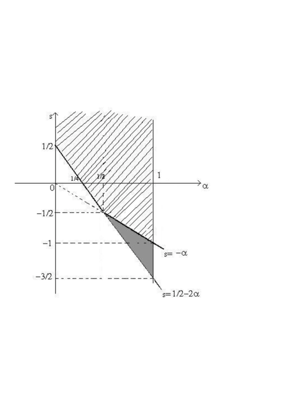
Figure 1. The domains of well-posedness and ill-posedness for the fractional heat equation (1.3) in $H^{s}({\TenEns R}),\;\alpha\,\in(0,1],\;s\in{\TenEns R}.$ Well-posedness holds inside the hatched region with its boundary without the point $(1/2,-1/2)$. Ill-posedness holds in side the shaded region and the point $(1/2,-1/2)$.

6.3. The periodic case

The periodic case can be treated in exactly the same way as the real line case since the linear fractional heat equation enjoys the same regularizing effects on the torus. The only difference is that the dilation symmetry, that we used at the end of Section 4, does not keep a torus invariant but maps it to another torus. To overcome this difficulty it suffices to notice that, in the periodic setting, the estimates derived in Section 3 are uniform for all period $\lambda\geq 1$.

References

- [1] I. Bejenaru and T. Tao, Sharp well-posedness and ill-posedness results for a quadratic non-linear Schrödinger equation, J. Funct. Anal. 233 (2006), 228–259.
- [2] J. Bourgain, Fourier restriction phenomena for certain lattice subset applications to nonlinear evolution equation, Geometric and Functional Anal., 3(1993), 107–156, 209–262.
- [3] H. Brézis and T. Cazenave, A nonlinear heat equation with singular initial data, J. Anal. Math., 68 (1996), 277-304.
- [4] T. Ghoul, An extension of Dickstein’s “small lambda” theorem for finite time blowup, Nonlinear Analysis, 74 (2011), 6105–6115.
- [5] Y. Giga, Solutions for semilinear parabolic equations in and regularity of weak solutions of the Navier-Stokes system, J. Differential Equations, 62 (1986), 186 212.
- [6] A. Haraux and F. B. Weissler, Non-uniqueness for a semilinear initial value problem, Indiana Univ. Math. J., 31 (1982), 167-189.
- [7] D. Henry, Geometric Theory of Semilinear Parabolic Equations, Lecture Notes in Mathematics, 840, Springer-Verlag, Berlin-New York, 1981.
- [8] T. Iwabuchi and T. Ogawa, Ill-posedness for nonlinear Schrödinger equation with quadratic non-linearity in lo dimensions, preprint.
- [9] L. Molinet, F. Ribaud and Y. Youssfi, Ill-posedness issues for a class of parabolic equations, Proc. Roy. Soc. Edinburgh Sect. A, 132 (2002), 1407–1416.
- [10] L. Molinet and S. Vento, Sharp ill-posedness and well-posedness results for the KdV-Burgers equation: the real line case, Ann. Scuola Norm. Sup. Pisa Cl. Sci. 10(2011), 531–560.
- [11] F. Ribaud, Cauchy problem for semilinear parabolic equations with initial data in spaces, Rev. Mat. Iberoamericana, 14 (1998), 1–46.
- [12] F. Ribaud, Semilinear parabolic equations with distributions as initial data, Discrete Contin. Dynam. Systems, 3 (1997), 305–316.
- [13] S. Snoussi, S. Tayachi, and F.B. Weissler, Asymptotically self-similar global solutions of a semilinear parabolic equation with a nonlinear gradient term, Proc. R. Soc. Edinb., Sect. A, Math. 129 (1999), 1291–1307.
- [14] S. Snoussi, S. Tayachi, and F.B. Weissler, Asymptotically self-similar global solutions of a general semilinear heat equation, Math. Ann., 321 (2001), 131–155.
- [15] Z. Tan and Y. Xu, Existence and nonexistence of global solutions for a semilinear heat equation with fractional laplacien, Acta Mathematica Scientia, Ser. B, 32(2012), 2203–2210.
- [16] D. Tataru, On global existence and scattering for the wave maps equation, Amer. J. Math. 123 (2001), 37–77.
- [17] M. E. Taylor, Pseudodifferential Operators and Nonlinear PDE, Progress in Mathematics, 100. Birkhaüser Boston, Inc., Boston, MA, 1991.
- [18] F. B. Weissler, Semilinear evolution equations in Banach spaces, J. Funct. Anal. 32 (1979), 277–296.
- [19] F. B. Weissler, Local existence and nonexistence for semilinear parabolic equation in , Indiana Univ. Math. J., 29 (1980), 79–102.
- [20] F. B. Weissler, Existence and nonexistence of global solutions for a semilinear heat equation, Israel J. Math., 38 (1981), 29–40.
- [21] J. Wu, Well-posedness of a semilinear heat equation with weak initial data, J. Fourier Anal. Appl., 4(1998), 629–642.