Production cross sections of $\gamma$-rays, electrons, and positrons in p-p collisions

Abstract

Because the production cross sections of $\gamma$ rays, electrons, and positrons (e^±) made in p-p collisions, $\sigma_{pp\rightarrow\gamma}$ and $\sigma_{pp\rightarrow{e}^{\pm}}$, respectively, are kinematically equivalent with respect to the parent pion-production cross section $\sigma_{pp\rightarrow\pi}$, we obtain $\sigma_{pp\rightarrow{e}^{\pm}}$ directly from the machine data on $\sigma_{pp\rightarrow\gamma}$. In Paper I (Sato et al. [1]), we give explicitly $\sigma_{pp\rightarrow\gamma}$, reproducing quite well the accelerator data with LHC, namely $\sigma_{pp\rightarrow{e}^{\pm}}$ is applicable enough over the wide energy range from GeV to 20 PeV for projectile proton energy. We dicuss in detail the relation between the cross sections, and present explicitly $\sigma_{pp\rightarrow{e}^{\pm}}$ that are valid into the PeV electron energy.

T. Shibata¹, Y. Ohira¹, K. Kohri², and R. Yamazaki¹

¹ Department of Physics and Mathematics, Aoyama-Gakuin University, Kanagawa 252-5258, Japan

² KEK Theory Center and the Graduate University for Advanced Studies (Sokendai) 1-1 Oho, Tsukuba 305-0801, Japan

1 Introduction.

Fluxes of cosmic-ray (CR) antimatter, namely antiprotons ($\bar{\rm p}$’s) and positrons (e⁺’s), have been measured with balloon and satellite experiments. Notable recent experiments in the higher-energy, $\stackrel{{\scriptstyle>}}{{\sim}}$ 100 GeV, regime, include PAMELA [2,3] and AMS-02 [4]. While the complete results of the latter experiment are not yet available, the improved accuracy of new CR data motivates new studies of the underlying production cross sections and collision kinematics.

Since the early reports around 1980 of the anomaly in the antiproton spectrum [5-7], cosmic-ray physics has shown itself in a position to test and potentially challenge conventional models in both particle physics and astrophysics. The antiproton anomaly in this experiment suffered, however, from limited sensitivity of the experiment, separation of atmospheric $\bar{\rm p}$’s, modulation effects, and low statistics.

The low-energy antiproton excess is not found in recent $\bar{\rm p}$ spectral data, for instance, BESS [8] and PAMELA [2], which gives data from $\sim 200$ MeV up to $\sim 100$ GeV. The $\bar{\rm p}$ spectrum is adequately explained by the standard model for the production of $\bar{\rm p}$ in the Galaxy and subsequent propagation to the Earth, within the uncertainties in the choice of model parameters.

Earlier, the HEAT (High Energy Antimatter Telescope) experiment [9] reported in 1995 a possible anomaly in the positron fraction. Connection of this excess to an explanation involving Weakly Interacting Massive Particles (WIMPs) has been suggested [10, 11]. DuVernois et al. [9] presented data indicating an excess of e⁺ in the higher energy region as compared to the expectation from the standard Galactic production and propagation models, and many antimatter searches have been performed since these early studies.

For instance, PAMELA [2, 12] recently reported with good statistics that the positron fraction increases with increasing energy above $\sim$ 4 GeV over the 0.1 – 150 GeV energy range. Fermi [13] also finds that the positron fraction in the 20-150 GeV is higher than expected from standard galactic propagations models. Both results indicate that the positron fraction rises significantly above 4 GeV up to 100 GeV.

AMS-02 will, in the near future, confirm the positron excess with higher statistics and unprecedented precision over a wide energy range from 0.5 GeV – 1 TeV [14]. It is particularly interesting to see if they observe a peak of the positron fraction around 350 GeV; the first result seems to be reaching a plateau at these energies [4].

The aim of the present paper is not to give an explanation for the anomaly in the positron spectrum, but rather to provide improved production cross sections for $\sigma_{pp\rightarrow s}(E_{0},E_{s})$ ($``s$” $\equiv$ $\gamma,\mbox{e}^{\pm}$, $\nu$) for decay product $s$ coming from pions produced in p-p collisions, and to present the kinematical relations between them. Here and in the following, $E_{0}$ and $E_{s}$ denote the laboratory frame (L.F.) kinetic energy of the projectile proton and the total energy of secondary s, respectively.

The parameterization for $\sigma_{pp\rightarrow\pi^{0}\rightarrow\gamma}$ has been studied by many authors [15-21], giving convenient forms for practical applications to the galactic phenomena. It is, however, experimentally very difficult to measure $\sigma_{pp\rightarrow\pi^{\pm}}$ for energetic charged pions produced by p-p collision in the high energy region. In fact, no data on $\sigma_{pp\rightarrow\pi^{\pm}}(E_{0},E_{\pi^{\pm}})$ are available above intersecting-storage-ring energies [22] with $E_{0}$ $\sim$ 1 TeV, before LHCf [23]. This is mainly due to the concentration of secondary products in the beam-fragmentation region that are too collimated to separate in the detector, in addition to the difficulty in energy determination of a single charged track with energy larger than $\approx 1$ TeV.

Previously, we have focused upon $\gamma$-ray production via $\pi^{0}$ instead of $\pi^{\pm}$, the energy determination of which is rather easy and reliable even in the high-energy region, $\stackrel{{\scriptstyle>}}{{\sim}}$ TeV, once a calorimeter is set well behind the vertex point of p-p interaction. In practice, cosmic-ray beam data is often obtained with an emulsion chamber (EC), covering $E_{0}$ = 10 $\sim$ 300 TeV [24, 25]. The EC used in these references consists of approximately 2 m air-gap spacer between an artificial carbon target and the calorimeter, which is distant enough to separate each $\gamma$-ray core and measure simultaneously its shower energy using a nuclear emulsion plate.

Besides this data, we also use the recent LHCf data [26, 27] on the $\gamma$-ray production energy spectrum, $dN/dE_{\gamma}$. This data is taken in the forward cone with unprecedented precision by placing the calorimeter far away, $\approx$ 140m, from the vertex point of p-p interaction. These papers give $dN/dE_{\gamma}$ at two energies in the center of mass frame (C.M.F.), $\sqrt{s}$ = 900 GeV and 7 TeV, corresponding to L.F. energies of approximately $E_{0}$ = 400 TeV and 26 PeV, respectively.

With the use of these data in the higher energy region as well as other past machine data in the lower energy region $\stackrel{{\scriptstyle<}}{{\sim}}$ TeV, we have already presented $\sigma_{pp\rightarrow\gamma}(E_{0},E_{\gamma})$ empirically in Paper I [1]. In this paper, we apply our work to the production cross section $\sigma_{pp\rightarrow e^{\pm}}(E_{0},E_{e})$ of e^± in p-p collisions, taking both the isobar and pionization components into account, as discussed in Paper I. It is worth mentioning some points about the modeling of the nuclear interaction that were not treated in Paper I.

Historically, multiple meson production in p-p collisions was introduced using the fireball model [28-32]. Resonance production was modeled by isobar emission [33-35]. After these early works, Stecker [15,16] proposed a two-component model consisting of isobar (excited baryon) and pionization (fireball) components, and applied this model to the study of cosmic $\gamma$ rays. Phenomenological interpretation of these production processes are nowadays well understood in the framework of QCD, though we do not use that approach here.

The present model is based on a two-component model, but differs in some important respects from the model developed earlier. For instance, we do not consider the fine structure of individual resonances with various masses and widths, but approximate them by an excited baryon with effective mass $M_{\Delta}$ and a broad width given by ${\it\Gamma}_{\Delta}$, regarding isobaric production through a single giant resonance in nuclear physics. They are determined so that the experimental data on both the average multiplicity and the production cross section of secondary products are well reproduced, as discussed in detail in Section 4. In Section 5.2, we compare three cross sections thus obtained, $\sigma_{pp\rightarrow\gamma}$, $\sigma_{pp\rightarrow e^{+}}$, and $\sigma_{pp\rightarrow e^{-}}$, with those obtained by Dermer [19, 20], Kamae et al. [21] and PYTHIA-code [36]. Finally in Section 6, we discuss briefly the application of the present model to the calculations for the emissivity of positron, particularly taking nuclei effect into account.

2 Energy spectrum of pionization secondaries

2.1 Modified rapidity

Before going into the main subject where we obtain the various cross sections, we introduce the variable $\eta$ defined by

$$\vspace{-2mm}\eta=\frac{1}{2}\ln\frac{1+\beta}{1-\beta}=\ln(\gamma+\sqrt{\gamma^{2}-1}),$$

with $\beta=v/c$ and $\gamma\equiv 1/\sqrt{1-\beta^{2}}$. Here v is particle velocity (in the following, we refer to $\beta$ as particle speed).

The variable $\eta$ corresponds to the familiar rapidity y, which is defined by

$$y=\frac{1}{2}\ln\frac{1+\beta\cos\theta}{1-\beta\cos\theta},$$

where $\theta$ is the emission angle of the particle. As can be readily seen, $|\eta|$ is the maximum rapidity of the particle, which lies in the range $-|\eta|\leq y\leq|\eta|$. We therefore, for simplicity, call $\eta$ the rapidity in the following discussion.

For the numerical calculations, we use the second relation in Eq. (1), since the first expression diverges for $\beta\rightarrow 1$. Hence we define the modified rapidity variable

$$\eta_{s}\equiv\eta(\gamma_{s})=\ln(\gamma_{s}+\sqrt{\gamma_{s}^{2}-1}),$$

regarding it as a function of the Lorentz factor $\gamma_{s}$ of particle s. With the use of $\eta_{s}$ for the secondary particle s with mass $m_{s}$, we have well-known expressions for the energy and momentum in natural units ($c=1$), namely

$$E_{s}=m_{s}\cosh\eta_{s}\;,\ \ P_{s}=m_{s}\sinh\eta_{s},$$

and

$$d\eta_{s}=dE_{s}/P_{s}.$$

2.2 Pion decay products

We introduce a normalized energy distribution function of pions produced by p-p collision in the L.F., $\Phi(E_{0},E_{\pi})$, where $E_{0}$ is the kinetic energy of a projectile proton, and $E_{\pi}$ is the total energy of parent pions ($\equiv$ $\pi^{0},\,\pi^{\pm}$). Then the normalized energy distribution of decay product $``s"$ ($\equiv\gamma,\ \mu^{\pm}$), $\varphi(E_{0},\epsilon_{s})$, is given by [37, 38]

$$\vspace{-3mm}\varphi(E_{0},\epsilon_{s})=\int_{E_{\pi}^{-}}^{E_{\pi}^{+}}\frac{\Phi(E_{0},E_{\pi})}{1-\kappa_{s}^{2}}\frac{dE_{\pi}}{P_{\pi}},$$

with

$$\vspace{3mm}\frac{E_{\pi}^{\pm}}{E_{s}}=\frac{(1+\kappa_{s}^{2})\pm(1-\kappa_{s}^{2})\beta_{s}}{2\kappa_{s}^{2}},$$

where $\kappa_{s}={m_{s}}/{m_{\pi}}$, $P_{\pi}$ is the momentum of the parent pion, and $\epsilon_{s}$ ($E_{s}$) the kinetic (total) energy of decay product s. $E_{\pi}^{-}$ ($E_{\pi}^{+}$) is the minimum (maximum) energy of the parent pion to produce the decay product $s$ with energy $\epsilon_{s}$, while $E_{\pi}^{+}$ = $E_{0}$ for $E_{\pi}^{+}\geq E_{0}$.

Note that Eq. (4) holds even in the case of $\kappa_{s}=0$ with $[m_{s},\beta_{s}]$ $\rightarrow$ $[0,1]$ in $\pi^{0}\rightarrow 2\gamma$ decay. See Eq. (5) below for the explicit form of $E_{\pi}^{\pm}$ in such a decay mode. So $\varphi(E_{0},\epsilon_{s})$ is the important function to determine.

2.3 Energy spectrum of $\gamma$ rays in $\pi^{0}\rightarrow 2\gamma$ decay

As mentioned in the Introduction, it is difficult to determine the distribution function $\Phi(E_{0},E_{\pi})$ experimentally in the high energy region $E_{0}$ $\stackrel{{\scriptstyle>}}{{\sim}}$ 1 TeV. Thus we focus upon $\varphi(E_{0},\epsilon_{\gamma})$ instead of $\Phi(E_{0},E_{\pi})$. In Paper I [1], we presented an empirical form based upon the raw machine data on $\gamma$ rays without relating it back to the parent $\pi^{0}$.

First we present the variables $E_{\pi}^{\pm}$ appearing in Eqs. (3) and (4). For $``s"\equiv\gamma$, [39]

$$E_{\pi}^{-}=E_{\gamma}+\frac{\ m_{\pi^{0}}^{2}}{4E_{\gamma}},\ \ E_{\pi}^{+}=E_{0}.$$

Another expression for $E_{\pi}^{-}$ is

$$E_{\pi}^{-}=m_{\pi^{0}}\cosh{\eta}_{\gamma},$$

with

$${\eta}_{\gamma}=\ln(2E_{\gamma}/m_{\pi^{0}}),$$

which are useful for giving the upper and lower limits of pion energy in electron production, as discussed in the next section.

The production spectrum of $\gamma$ rays with average multiplicity $\bar{N}_{\gamma}(E_{0})$ is given by [1]

$$\frac{dN_{\gamma}}{dE_{\gamma}}=\bar{N}_{\gamma}(E_{0})\varphi(E_{0},\epsilon_{\gamma}),$$

with

$$\frac{\varphi(E_{0},\epsilon_{\gamma})}{\beta_{c}^{2}{\it\Theta}_{c}}=\frac{1}{M_{p}}\int_{\omega_{-}}^{\omega_{+}}\frac{(1-x_{\gamma}{\it\Gamma}_{\theta})^{4}}{{\it\Gamma}_{\theta}+\zeta\tau_{\theta}}\mbox{e}^{-\tau_{\theta}x_{\gamma}}d\omega.$$

Here $\omega=\cos\theta$, and

$$x_{\gamma}=\frac{E_{\pi}^{-}}{E_{0}}=\frac{E_{\gamma}}{E_{0}}\biggl{[}1+\frac{m_{\pi^{0}}^{2}}{4E_{\gamma}^{2}}\biggr{]},$$

with

$$\vspace{2mm}\omega_{\pm}=\beta_{c}^{-1}-\beta_{c}^{\pm 1}\mbox{e}^{\pm\eta_{0}^{*}-\eta_{\gamma}^{*}},$$

$$\eta_{0}^{*}=\ln(2\beta_{c}\gamma_{c}{M_{p}}/{m_{\pi^{0}}}),$$

$$\vspace{2mm}\eta_{\gamma}^{*}=\ln(2\beta_{c}\gamma_{c}{E_{\gamma}}/{m_{\pi^{0}}}).$$

Here $\beta_{c}$ ($\gamma_{c}$) is the velocity (Lorentz factor) of the C.M.F. with respect to the L.F., ${\it\Theta}_{c}$ is the normalization constant given by Eq. (A2), and $M_{p}$ the mass of proton; see Appendix A for $[\tau_{\theta},{\it\Gamma}_{\theta}]$ and $[{\it\Theta}_{c},\zeta]$. In Eq. (11), $\omega_{-}=-1$ for $E_{\gamma}<\frac{1}{2}m_{\pi^{0}}\mbox{e}^{-(\eta_{0}^{*}+\eta_{c})}$ (note that $\eta_{c}$ is the rapidity of the C.M.F. as measured in the L.F., and $\eta_{c}$ $\equiv$ $\eta(\gamma_{c})$ in Eq. [2]).

2.4 Energy spectra of $\mbox{e}^{\pm}$ via $\pi^{\pm}$- $\mu^{\pm}$- $\mbox{e}^{\pm}$ decay

An electron (positron) with energy $\check{E}_{e}$ is created following three-body decay of a fully polarized muon in the decay $\mu^{\pm}\rightarrow\mbox{e}^{\pm}+\nu_{e}(\bar{\nu}_{e})+\bar{\nu}_{\mu}({\nu}_{\mu})$. The production of $\mu^{\pm}$ is kinematically equivalent to the production of $\gamma$ rays because the two-body decay is isotropic, as discussed in Section 2.2.

The energy/angular distribution of electrons (positrons) in the muon rest frame is given by [51-53]

$$\vspace{1mm}\check{f}(\check{q},\check{\theta})=\check{q}^{2}(3-2\check{q})\biggl{[}1+\xi\cos\check{\theta}\frac{1-2\check{q}}{3-2\check{q}}\biggr{]},$$

where $\check{q}=2\check{E}_{e}/m_{\mu}$, $\xi=+1$ ($-1$) for electrons (positrons), and $\check{\theta}$ is the angle between the electron (positron) and the spin of the muon in the muon rest frame. Eq. (13) is valid also for muon neutrinos $\nu_{\mu}$ in the approximation that the electron mass $m_{e}$ is neglected. For the electron neutrino $\nu_{e}$, both ($3-2\check{q}$) and ($1-2\check{q}$) in Eq. (13) are replaced by $6(1-\check{q})$ [53].

In practice we need the energy distribution of $\mbox{e}^{\pm}$, $f(E_{\pi},E_{e})$, for a parent pion with the fixed energy $E_{\pi}$ in the L.F.. The full expression for $f(E_{\pi},E_{e})$, which is tedious to evaluate, is summarized by Dermer ([19]; see also Moskalenko & Strong [54]).

For the pion rapidity $\eta_{\pi}$, we introduce a function $\phi(\eta_{\pi},q_{e})$ defined by

$$\phi(\eta_{\pi},q_{e})={P_{\pi}}f(E_{\pi},E_{e}),$$

and in Table 1 we summarize it explicitly with the use of three parameters, $[q_{e},\eta_{\pi},\tilde{\eta}_{\mu}]$, which are given by

$$q_{e}=2E_{e}/m_{\mu},$$

and

$$\vspace{3mm}E_{\pi}=m_{\pi}\cosh\eta_{\pi},$$

with $\eta_{\pi}\equiv\eta(\gamma_{\pi})$, and $\tilde{\eta}_{\mu}\equiv\eta(\tilde{\gamma}_{\mu})$ in Eq. (2). The term $q_{e}$ is the L.F. electron (positron) energy $E_{e}$, in units of half of the muon mass, $\frac{1}{2}m_{\mu}$. Two rapidity variables, $\eta_{\pi}$ and $\tilde{\eta}_{\mu}$, correspond to those of the parent pion in the L.F.  and the daughter muon in the pion rest frame, respectively. Since $\tilde{\gamma}_{\mu}=\frac{1}{2}(m_{\mu}/m_{\pi}+m_{\pi}/m_{\mu})=1.04$, we find $\tilde{\eta}_{\mu}=0.278$ with $\tilde{\beta}_{\mu}=0.271$, and $[g_{0};\ g_{1,0}$, $g_{2,0}]$ in Table 1 equal [1.16; 3.75, 6.78] for $\xi$ = 1 (electron), and [-0.57; 4.49, 1.03] for $\xi$ = -1 (positron), respectively.

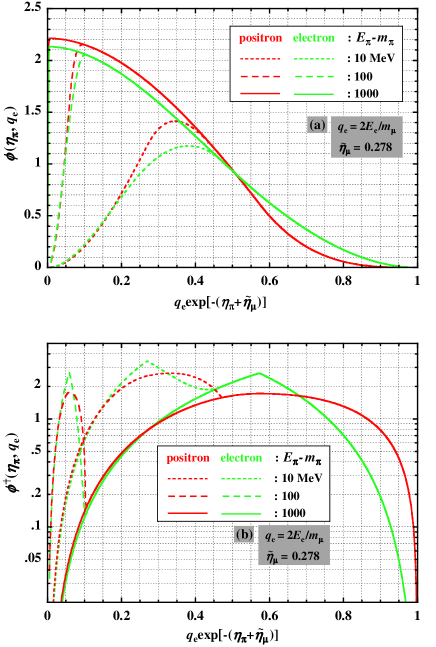
Figure 1: Numerical values for (a) $\phi(\eta_{\pi},q_{e})$ and (b) $\phi^{\dagger}(\eta_{\pi},q_{e})$. For $\epsilon_{\pi}(\equiv E_{\pi}-m_{\pi})$ larger than 1 GeV, both $\phi$ and $\phi^{\dagger}$ scale in the forms of $\phi(E_{e}/E_{\pi})$ and $\phi^{\dagger}(E_{e}/E_{\pi})$, respectively, as $q_{e}\exp(-\eta_{\pi})\approx E_{e}/E_{\pi}$.

In Fig. 1a, we present numerical values of $\phi(\eta_{\pi},q_{e})$ vs. $q_{e}\exp[-(\eta_{\pi}+\bar{\eta}_{\mu})]$ for three pion kinetic energies $\epsilon_{\pi}$ ($\equiv$ $E_{\pi}-m_{\pi}$) = 0.01, 0.1, and 1 GeV in the case of electrons (green curves) and positrons (red curves). For $\epsilon_{\pi}$ $\stackrel{{\scriptstyle>}}{{\sim}}$ 1 GeV, one finds $\phi(\eta_{\pi},q_{e})$ $\approx$ $\phi(q_{e}\mbox{e}^{-\eta_{\pi}})$. Hence in the high energy region, $q_{e}\mbox{e}^{-\eta_{\pi}}\approx E_{e}/E_{\pi}$, so that $\phi(\eta_{\pi},q_{e})\approx\phi(E_{e}/E_{\pi})$.

The normalization in Eq. (14) holds exactly, taking care that the restriction $q_{e}\subseteq[q_{e}^{-},q_{e}^{+}]$ in Table 1, namely

$$\int_{E_{e}^{-}}^{E_{e}^{+}}\phi(\eta_{\pi},q_{e})\frac{dE_{e}}{P_{\pi}}=1,$$

where

$$\vspace{1mm}E_{e}^{-}=0;\ \ 2E_{e}^{+}=m_{\mu}\mbox{e}^{\eta_{\pi}+\tilde{\eta}_{\mu}},$$

is satisfied.

Once we have the normalized energy spectrum of $\mbox{e}^{\pm}$ coming from the $\pi^{\pm}$-$\mu^{\pm}$-${\rm e}^{\pm}$ decay in the L.F., we can straightforwardly obtain the production energy spectrum of $\mbox{e}^{\pm}$ in p-p collisions (see Eq. [3] for $\Phi$), through the expression

$$\frac{dN_{e^{\pm}}}{dE_{e}}=\bar{N}_{\pi^{\pm}}\!\!\int_{E_{\pi}^{-}}^{E_{\pi}^{+}}\!\Phi(E_{0},E_{\pi})f(E_{\pi},E_{e})dE_{\pi},$$

where

$$\vspace{1mm}E_{\pi}^{\pm}=m_{\pi}\cosh\eta_{\pi}^{\pm}.$$

Here $\bar{N}_{\pi^{\pm}}(E_{0})$ is the effective multiplicity of charged pions, which depends on the projectile proton energy $E_{0}$, and

$$\eta_{\pi}^{-}=\bar{\eta}_{e}-\tilde{\eta}_{\mu};\ \ \eta_{\pi}^{+}=\bar{\eta}_{\pi}^{*}+\eta_{c}.$$

Here $\bar{\eta}_{e}=\ln q_{e}$, and $\bar{\eta}_{\pi}^{*}$ is the maximum C.M.F. rapidity of pions given by Eq. (A3) in Appendix A, and $\eta_{\pi}^{+}$ is the maximum pion rapidity in the L.F..

Another expression for $E_{\pi}^{-}$ in Eq. (17) is given by

$$E_{\pi}^{-}=E_{e}+\frac{m_{\pi}^{2}}{4E_{e}},$$

which is similar to Eq. (5) for the $\gamma$-ray energy spectrum.

Noting the relation between $\varphi$ and $\Phi$ given by Eq. (3) with $E_{\pi}^{-}(\epsilon_{\gamma})$ in the case of $\pi^{0}\rightarrow 2\gamma$ decay, we have 

$$\vspace{3mm}\frac{\partial\varphi}{\partial\epsilon}\biggr{|}_{\epsilon=E_{\pi}-m_{\pi}}=-\Phi(E_{0},E_{\pi})\frac{1}{P_{\pi}},$$

and using Eq. (14) together with the relation $dE_{\pi}/P_{\pi}=d\eta_{\pi}$, eventually we obtain

$$\frac{dN_{e^{\pm}}}{dE_{e}}={\bar{N}_{\pi^{\pm}}}\!\int_{\eta_{\pi}^{-}}^{\eta_{\pi}^{+}}\!\varphi(E_{0},\epsilon_{\pi})\phi^{\dagger}(\eta_{\pi},q_{e})d\eta_{\pi},$$

where $\phi^{\dagger}(\eta_{\pi},q_{e})$ denotes the differential of $\phi(\eta_{\pi},q_{e})$ with respect to $\eta_{\pi}$. An explicit form of $\phi^{\dagger}(\eta_{\pi},q_{e})$ is presented in Table 1 together with $\phi(\eta_{\pi},q_{e})$. See Eq. (18) for $\eta_{\pi}^{\pm}$, recalling that $\epsilon_{\pi}$ ($\equiv E_{\pi}-m_{\pi}$) is the L.F. kinetic energy of pion expressed in terms of $\eta_{\pi}$ as

$$\epsilon_{\pi}=2m_{\pi}\sinh^{2}\frac{\eta_{\pi}}{2}.$$

Fig. 1b shows numerical values of $\phi^{\dagger}(\eta_{\pi},q_{e})$ vs. $q_{e}\exp[-(\eta_{\pi}+\bar{\eta}_{\mu})]$, for the same three parent pion kinetic energies used in Fig. 1a. We find again a scaling behavior of $\phi^{\dagger}(E_{e}/E_{\pi})$ similar to $\phi(E_{e}/E_{\pi})$ in the high energy region $\epsilon_{\pi}\ \mbox{\raisebox{-4.30554pt}{$\stackrel{{\scriptstyle>}}{{\sim}}$}}\ 1$ GeV.

3 Energy spectrum of secondary products in isobaric resonances

In the low energy region around $E_{0}\cong 1$ – 3 GeV in p-p collisions, many isobaric resonances, such as ${\it\Delta}(1232)$, ${\it\Delta}(1410),\ldots$ , as well as the exclusive channel $pp\rightarrow\pi^{+}d$ ($d$: deuteron) become effective for secondary production in addition to those coming from the pionization component mentioned in the last section. In this section we consider an expression for the production cross section of secondaries that approximately reproduces the experimental data, particularly for $\pi^{0}$ and $\pi^{+}$. This does not necessarily give a good representation for other mesons, such as $\pi^{-}$ and K^± (see Figs. 2a and 2b), but the contributions of which are negligibly small comparing to those of $\pi^{0}$ and $\pi^{+}$.

3.1 Energy spectrum of $\gamma$ rays via $\Delta$ - $\pi^{0}$- $2\gamma$ decay

We assume that an isobar with mass $M_{\Delta}$ is produced in p-p collision, and disintegrates isotropically into $\pi^{0}$ (+ $p$) or $\pi^{+}$ (+ $n$) with pion energy $\hat{E}_{\pi}$ in the isobar rest frame. This implies

$$\hat{E}_{\pi}=m_{\pi}\tau_{\Delta}\cosh\hat{\eta}_{\Delta},$$

with

$$\hat{\eta}_{\Delta}=\ln(\tau_{\Delta}M_{\Delta}/m_{\pi});\ \ \tau_{\Delta}=\sqrt{1-M_{p}^{2}/M_{\Delta}^{2}}.$$

In the calculations, we set $M_{\Delta}$ = 1.25 GeV/c² with $\tau_{\Delta}=0.66$ (see Sec. [4.1]), so that numerical values of the decaying pion in the isobar rest frame, $\hat{E}_{\pi}$, $\hat{P}_{\pi}$ (momentum), $\hat{\beta}_{\pi}$ (velocity), $\hat{\gamma}_{\pi}$ (Lorentz factor), and $\hat{\eta}_{\pi}$ (rapidity), are given by

$$[\hat{E}_{\pi},\ c\hat{P}_{\pi}]=[279,\ 242]~{}\mbox{MeV},$$

and

$$[\hat{\beta}_{\pi},\hat{\gamma}_{\pi},\hat{\eta}_{\pi}]=[0.87,2.01,1.32],$$

respectively.

One might argue that there are many resonances disintegrating into $\pi^{0}$ or $\pi^{\pm}$, in contrast with a single resonance with $M_{\Delta}$ = 1.25,GeV/c² assumed here. As emphasized in the Introduction, however, we do not consider the fine structure or mass spectrum of individual resonances, but approximate resonance production in terms of something like a giant resonance (well-known in nuclear physics), the width of which is determined so that the experimental data are consistently reproduced with Eq. (29). Moreover, even in more detailed treatments that employ a Breit-Wigner distribution for the resonance mass spectrum, there is an implicit assumption that the excited nucleon travels in its original, pre-collision direction. This may be a good assumption for low-momentum transfer, peripheral collisions.

Therefore, the energy distribution of pions via isobar disintegration in the L.F. can be written as

$$\vspace{2mm}\Phi_{\Delta}(E_{0},E_{\pi})dE_{\pi}=\Phi_{0}(E_{0})dE_{\pi},$$

and $\Phi_{0}$ is determined from the normalization bound to $\hat{E}_{\pi}^{-}\leq E_{\pi}\leq\hat{E}_{\pi}^{+}$ with

$$\hat{E}_{\pi}^{\pm}=\gamma_{\Delta}^{*}\gamma_{c}[(1+\beta_{c}\beta_{\Delta}^{*})\pm(\beta_{c}+\beta_{\Delta}^{*})\hat{\beta}_{\pi}]\hat{E}_{\pi},$$

where $\gamma_{\Delta}^{*}$ ($\beta_{\Delta}^{*}$) is Lorentz factor (velocity) of the isobar in C.M.F. given by

$$\gamma_{\Delta}^{*}=\tau_{\Delta}\cosh\eta_{s}^{*};\ \ \eta_{s}^{*}=\ln(\sqrt{s}/\tau_{\Delta}M_{\Delta}),$$

and $\sqrt{s}=2M_{p}\gamma_{c}$ is the center of mass energy.

Using isobar rapidities $\eta_{\Delta}$ and $\eta_{\Delta}^{*}$, in the L.F. and C.M.F. respectively, we have a simple and physically trivial expression,

$$\hat{E}_{\pi}^{\pm}=m_{\pi}\cosh(\eta_{\Delta}\pm\hat{\eta}_{\pi}),$$

with

$$\eta_{\Delta}=\eta_{\Delta}^{*}+\eta_{c}\equiv\eta(\gamma_{\Delta}^{*})+\eta_{c}.$$

Now, the normalization constant $\Phi_{0}(E_{0})$ in Eq. (23) is given by

$$\Phi_{0}(E_{0})=\frac{1}{2\hat{P}_{\pi}}\frac{1}{\sinh\eta_{\Delta}}.$$

and from Eq. (3), we can write the production energy spectrum of $\gamma$ rays coming from the isobaric resonances with $[E_{\pi}^{-},E_{\pi}^{+}]$ given by Eq. (5), namely

$$\varphi_{\Delta}(E_{0},\epsilon_{\gamma})=\int_{E_{\pi}^{-}}^{E_{\pi}^{+}}\!\!{\Phi_{\Delta}(E_{0},E_{\pi})}\frac{dE_{\pi}}{P_{\pi}}.$$

Using the relation $d\eta=dE_{\pi}/P_{\pi}$, finally we have a simple form

$$\frac{dN_{\gamma}^{\Delta}}{dE_{\gamma}}=\frac{\bar{N}_{\gamma}^{\Delta}}{2\hat{P}_{\pi}\sinh\eta_{\Delta}}[\eta_{p}-\eta_{\gamma}],$$

where ${\bar{N}_{\gamma}^{\Delta}}$ is the effective multiplicity of $\gamma$-rays (via $\pi^{0}$) through the $\Delta$-isobar disintegration, and $\eta_{p}$ is the rapidity of projectile proton given by Eq. (2) with $\eta_{p}\equiv\eta(\gamma_{p})$, with $\gamma_{p}=1+E_{0}/M_{p}$, and $\eta_{\gamma}$ the minimum rapidity of pion given by Eq. (7) to produce $\gamma$ rays with energy $E_{\gamma}$ (= $\epsilon_{\gamma}$).

3.2 Energy spectrum of e⁺ via $\Delta$ - $\pi^{+}$- $\mu^{+}$- $\mbox{e}^{+}$ decay

As the contribution of $\pi^{-}$ from the isobaric resonance in p-p collision is negligible in comparison with $\pi^{+}$ around a few GeV (see Fig. 2b), we consider here the energy spectrum of e⁺ via $\pi^{+}$- $\mu^{+}$- $\mbox{e}^{+}$ decay only.

Similar to Eq. (16), we obtain the production energy spectrum of e⁺ coming from the isobar decay, $\Delta$ $\rightarrow$ $\pi^{+}$$\rightarrow$ $\mu^{+}$ $\rightarrow$ $\mbox{e}^{+}$, namely

$$\frac{dN_{e^{+}}^{\Delta}}{dE_{e}}=\bar{N}_{\pi^{+}}^{\Delta}\!\!\int_{E_{\pi}^{-}}^{E_{\pi}^{+}}\!\Phi_{\Delta}(E_{0},E_{\pi})f(E_{\pi},E_{e})dE_{\pi},$$

where $\bar{N}_{\pi^{+}}^{\Delta}$ is the effective multiplicity of $\pi^{+}$ through the disintegration of the $\Delta$-isobar, noting Eq. (17) for $E_{\pi}^{\pm}$.

With the use of $\Phi_{0}(E_{0})$ given by Eq. (25) in $\Phi_{\Delta}(E_{0},E_{\pi})$, we obtain

$$\vspace{2mm}\frac{dN_{e^{+}}^{\Delta}}{dE_{e}}=\frac{\bar{N}_{\pi^{+}}^{\Delta}}{2\hat{P}_{\pi}\sinh\eta_{\Delta}}\!\int_{\eta_{\pi}^{-}}^{\eta_{\pi}^{+}}\!\!{\phi(\eta_{\pi},q_{e})d\eta_{\pi}},$$

where $\eta_{\pi}^{\pm}$ are given by Eqs. (18) and (A3).

Here it is important to take care that the integration with respect to $\eta_{\pi}$ in the above equation, which must be performed separately over the allowed range of $\eta_{\pi}$, depending on positron energy $E_{e}\ (=\frac{1}{2}m_{\mu}q_{e})$; see the restriction $q_{e}\subseteq[q_{e}^{-},q_{e}^{+}]$ in Table 1. Note also that the energy spectra of secondary $\gamma$ rays and $\mbox{e}^{+}$ coming from both pionization and isobaric components given by Eqs. (8), (21), (26) and (27), are all expressed only by $\phi$, $\phi^{\dagger}$, and $\int\!\phi\,d\eta_{\pi}$, apart from the basic function $\varphi(E_{0},\epsilon)$ for the pionization components in Eqs. (8) and (21). In the next section, explicit numerical values of the parameters appearing above, $M_{\Delta},\ \bar{N}_{\gamma}^{\Delta}$, etc., are given.

4 Multiplicity of secondary particles

We presented in the previous section the production energy spectra of $\gamma$ rays and $\mbox{e}^{\pm}$ in p-p collisions, [$dN_{\gamma}/{dE_{\gamma}}$, $dN_{e^{\pm}}/{dE_{e}}$] from the pionization components, and [$dN_{\gamma}^{\Delta}/{dE_{\gamma}}$, $dN_{e^{+}}^{\Delta}/{dE_{e}}$] from the isobaric ones, respectively. For these spectra, we need the average multiplicity of secondaries per p-p collision, [$\bar{N}_{\gamma}$, $\bar{N}_{\pi^{\pm}}$] for the former components, and [$\bar{N}_{\gamma}^{\Delta}$, $\bar{N}_{\pi^{+}}^{\Delta}$] for the latter ones, respectively, each depending on the energy of projectile proton $E_{0}$. These numerical values should be determined from the machine data.

Here, as noted also in Paper I, the multiplicity should be regarded as an effective one rather than an actual one, particularly in the high energy region, since the low-energy secondaries produced in the backward cone in the C.M.F. in p-p collision do not make a signficant contribution to the total secondaries formed in the galactic CR system.

4.1 Parameterization of the empirical formulae

In this paper, we modify slightly the average multiplicity of $\gamma$’s, $\bar{N}_{\gamma}(E_{0})$, presented in Paper I, since those coming from isobar decay, such as $\bar{N}_{\gamma}^{\Delta}(E_{0})$ from $\pi^{0}$ + p given by Eq. (29) below, are additionally included in the present work. Hence the total average multiplicity, $\bar{N}_{\gamma}$ + $\bar{N}_{\gamma}^{\Delta}$, must be fitted to the machine data in contrast to the fitting without $\bar{N}_{\gamma}^{\Delta}$ in Paper I.

We assume that the energy dependence on the average multiplicities of $\pi^{\pm}$ and K^± are of the same form as in the case of $\gamma$ rays, for both pionization and isobar components, $\bar{N}_{s}(E_{0})$ and $\bar{N}_{s}^{\Delta}(E_{0})$ ($``s"\,\equiv\,\gamma,\pi^{\pm},\mbox{K}^{\pm}$), respectively, but with different numerical values in the parameterization for each term as discussed below.

First, we summarize the multiplicity coming from the pionization component, slightly modifying the parameterization in Paper I, now in the form

$$\bar{N}_{s}(E_{0})=\bar{N}_{0}{\it\Lambda}_{s}({\epsilon}_{0}){\epsilon}_{0}^{\,0.115},$$

with

$${\epsilon}_{0}=E_{0}-E_{\rm th},$$

and

$${\it\Lambda}_{s}(\epsilon_{0})=\Bigl{[}1-\mbox{e}^{-\sqrt{\epsilon_{0}/\epsilon_{1}}}\Bigr{]}\Bigl{[}1-\mbox{e}^{-\sqrt[4]{\epsilon_{0}/\epsilon_{2}}}\Bigr{]}\mbox{e}^{-(\epsilon_{c}/\epsilon_{0})^{k}},$$

where numerical values of $\bar{N}_{0}$, $E_{\rm th}$, $\epsilon_{c}$, and $k$ are presented in Table 2 for individual secondaries, $``s$” $\equiv$ $\gamma,~{}\pi^{\pm},\mbox{K}^{\pm}$, while $[\epsilon_{1},\epsilon_{2}]$ = [4.53 GeV, 1.98 TeV] irrespective of s.

Second, for the multiplicity of $\gamma$ rays and $\pi^{+}$ through the disintegration of a $\Delta$ isobar, we assume

$$\vspace{1mm}\bar{N}_{s}^{\Delta}(E_{0})=\bar{N}_{0}^{\Delta}\mbox{exp}\biggl{[}-\biggl{\{}\frac{\ln({\epsilon}_{0}/M_{\Delta})}{\ln m_{\pi}}\biggr{\}}^{2}\biggr{]},$$

where $m_{\pi}$ is the pion mass in GeV/c², and $\bar{N}_{0}^{\Delta}$ = [0.61, 0.25] for $``s"\equiv$ [$\pi^{+},\gamma$] respectively. One can regard the exponential function in Eq. (29) as the width in $\ln M_{\Delta}$-scale of the $\Delta$ isobar with the mass $M_{\Delta}$ instead of the Breit-Wigner type function.

We assume $M_{\Delta}$ = 1.25 GeV/c², leading to [$\hat{E}_{\pi},\hat{\eta}_{\pi}$] = [0.279 GeV, 1.32] as presented in Section 3.1. These numerical values are determined so that the experimental data on the total production cross sections of $\gamma$ rays, $\pi^{\pm}$, and K^±, as presented in Figs. 2a and 2b, are reproduced.

4.2 Comparison with total production cross section data

The total production cross section, $\sigma_{pp\rightarrow s}^{tot}$, to produce a secondary $``s$” coming from both pionization and isobar components is given by $\sigma_{inel}\times(\bar{N}_{s}+\bar{N}_{s}^{\Delta})$, where $\sigma_{inel}$ is the total inelastic collision cross section, including all collisions except elastic one. In the following, we simply rewrite $\bar{N}_{s}$ + $\bar{N}_{s}^{\Delta}$ with $\bar{N}_{s}$, unless mentioned specifically, and regard, for simplicity, $\bar{N}_{s}$ as the total average multiplicity of the element s. The explicit form of $\sigma_{inel}$ is given by Eqs. (1) and (2) in Paper I, covering from the threshold energy of pion production to the LHC energy.

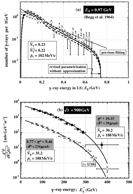
Figure 4: (a) Production cross section of $\gamma$ rays at $E_{0}$ = 0.97 GeV, where we present empirical ones both from the old one (dotted curve) and the revised one (heavy solid one). (b) Production cross section of $\gamma$ rays at $\sqrt{s}$ = 900 GeV, corresponding to $E_{0}\approx$ 400 TeV, where solid curvess are obtained by the present empirical ones.

In Figs. 2a and 2b we show historical data ([1, 16, 19, 55, 56]) on $\sigma_{pp\rightarrow s}^{tot}$ for $\gamma$ rays (a) and charged mesons (b). Here, broken curves correspond to those coming from isobar component alone, $\sigma_{inel}\times\bar{N}_{s}^{\Delta}$, see Eq. (29) for $\bar{N}_{s}^{\Delta}$, and the solid ones from the summed cross sections, $\sigma_{inel}\times(\bar{N}_{s}$ + $\bar{N}_{s}^{\Delta})$, see Eq. (28) with Table 2 for $\bar{N}_{s}$. Additionally plotted by blue circles is the very high energy LHC data with $\sqrt{s}$ = 900 GeV, 7 TeV (Paper I [1]). In Fig. 4b of Appendix A, we demonstrate an example of this model by fitting recent data at $\sqrt{s}$ = 900 GeV [57]. See Paper I for a more complete comparison, including pseudo-rapidity, Feynman variable, $\gamma$-ray energy, and so on, in both the C.M.F. and L.F., covering very wide energies up to LHC energies, ranging from $E_{0}$ = $1\,\mbox{GeV}$ to $\approx 20\,\mbox{PeV}$.

Fig. 2b shows that the contribution of K^± is on average as large as 7% by total number of charged mesons made when $E_{0}$ $\stackrel{{\scriptstyle>}}{{\sim}}$ 10 GeV, and negligible below, so that the contribution to e^± coming from K^± could be at most 7%, and smaller after decay kinematics are taken into account. Thus, in the numerical calculations, we consider only $\pi^{\pm}$’s as the source of secondary e^±’s, but assume 7% increase in the absolute intensities of secondary e^±’s we are interested in due to kaon contribution.

5 Comparison with other numerical codes for the elementary processes

Many quite elaborate codes for the treatment of secondary nuclear production processes, with applications to CRs and galactic phenomena, have been developed ([19, 20, 21, 36, 54]). Accurate cross sections and production spectra become increasingly important as new observational data from Fermi and AMS-02 become available with high quality in both statistics and systematics. In this section, we compare our calculations for the production cross sections of $\gamma$ rays and $\mbox{e}^{\pm}$ in p-p collision with those calculated by (a) Dermer [19], (b) Kamae et al. [21], and the (c) PYTHIA-code (Sjostrand [36]).

In order to compare their calculations with the present ones, we summarize the notations for the production cross section of individual elements in the followings,

$$\frac{d\sigma}{dE_{\gamma}}(E_{0},E_{\gamma})=\sigma_{inel}\biggl{(}\frac{dN_{\gamma}}{dE_{\gamma}}+\frac{dN_{\gamma}^{\Delta}}{dE_{\gamma}}\biggr{)},$$

for $\gamma$ rays,

$$\frac{d\sigma}{dE_{e}}(E_{0},E_{e})=\sigma_{inel}\biggl{(}\frac{dN_{e^{+}}}{dE_{e}}+\frac{dN_{e^{+}}^{\Delta}}{dE_{e}}\biggr{)},$$

for positrons, and

$$\vspace{2mm}\frac{d\sigma}{dE_{e}}(E_{0},E_{e})=\sigma_{inel}\frac{dN_{e^{-}}}{dE_{e}},$$

for electrons. See Paper I for $\sigma_{inel}$.

Explicit equations used for the calculations of the spectra in the right hand side correspond to following relations:

$$\biggl{[}\frac{dN_{\gamma}}{dE_{\gamma}},\ \frac{dN_{\gamma}^{\Delta}}{dE_{\gamma}}\biggr{]}\Rightarrow[{\rm Eq.\ 8},\ {\rm Eq.\ 26}],$$

$$\vspace{2mm}\biggl{[}\frac{dN_{e^{\pm}}}{dE_{e}},\ \frac{dN_{e^{+}}^{\Delta}}{dE_{e}}\biggr{]}\Rightarrow[{\rm Eq.\ 21},\ {\rm Eq.\ 27}].$$

5.1 Production cross section of $\gamma$ rays

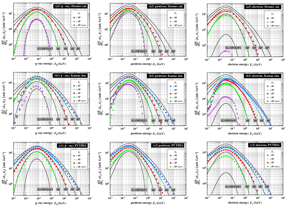
Figure 3: Comparisons of the present production cross sections (heavy solid curves) for (a1-c1) $\sigma_{pp\rightarrow\gamma}$, (a2-c2) $\sigma_{pp\rightarrow e^{+}}$, and (a3-c3) $\sigma_{pp\rightarrow e^{-}}$, with others (square symbols) by (a1-a3) Dermer [19], (b1-b3) Kamae et al. [21], and (c1-c3) PYTHIA (Sjostrand et al. [36]), for $E_{0}$ = $10^{0},10^{1},10^{2},10^{3},10^{4}$ GeV.

Figs. 3(a1-c1) show our numerical results on the production cross section of $\gamma$ rays in p-p collision (heavy solid curves) in comparison with numerical results by (a) Dermer [19] and Murphy et al. [41], (b) Kamae et al. [21] and Karlsson & Kamae [41], and the (c) PYTHIA-code [36], for $E_{0}$ = $10^{0},10^{1},10^{2},10^{3},10^{4}$ GeV. Note that Murphy et al. presents results only up to $E_{0}$ = $10^{2}$ GeV, and PYTHIA is not applicable at low, $E_{0}\,\mbox{\raisebox{-4.30554pt}{$\stackrel{{\scriptstyle<}}{{\sim}}$}}$ 1 GeV, energies.

As can be seen, the models are in general agreement. Below 1 GeV, however, our model with the simplified treatment of resonance production deviates from the Kamae et al. model, but is in good agreement with the Murphy et al. calculations. Note also that Kamae model is not symmetric about $\frac{1}{2}m_{\pi^{0}}\approx 70$ MeV when plotted vs $\ln E_{\gamma}$, while it must be kinematically symmetric as is well-known.

Small but significant deviations are also seen in the production spectra when $E_{0}\,\mbox{\raisebox{-4.30554pt}{$\stackrel{{\scriptstyle>}}{{\sim}}$}}\,1\,$TeV, increasing with energy. These differences, which would earlier be masked by the large observational uncertainties, are now important when treating secondary particles produced by CR/ISM collisions. Machine data used in past models focused on the energy range $E_{0}\,\mbox{\raisebox{-4.30554pt}{$\stackrel{{\scriptstyle<}}{{\sim}}$}}\,$TeV, while this range is now becoming important due to the improved high-energy CR data. Fig. 4b in Appendix A is an example of the comparison between the present parameterization and the most recent LHCf data [57] on the production energy spectrum of $\gamma$ rays.

Ground-based very-high-energy $\gamma$-ray astronomy, overlapping with Fermi-LAT in the energy range between $\approx 50$ – 200 GeV, will provide additional relevant data. For example, H.E.S.S., besides discovering many new TeV sources, has also recently announced the detection of diffuse $\gamma$ rays in the TeV region around the galactic plane [42]. Furthermore, the full observation program by the Cherenkov Telescope Array (CTA) will start around 2020 [43], so that the LHC data at TeV energies and higher becomes increasingly relevant to analysis of TeV $\gamma$-ray data.

5.2 Production cross section of $\mbox{e}^{\pm}$

Figs. 3(a2-c2) and 3(a3-c3) show production cross sections of positrons and electrons in p-p collisions, respectively. Our results are similar to those by Dermer [19] and Murphy et al. [41] in the low-energy regime for e⁺ production, though not for electrons at $E_{0}=1$ GeV in Fig. 3(a3), which however make a very minor contribution to lepton production. We again find that there exists a significant discrepancy between ours and other models in the high-energy, $E_{0}\gg 100$ GeV, regime.

Unfortunately, we have no user-friendly experimental data on the production of secondary electrons (positrons) via $\pi$-$\mu$ decay. However, as emphasized in Section 2, the cross sections for $\gamma$ and $\mbox{e}^{\pm}$ production are linked through the $\pi^{\pm}$-decay kinematics. So the reliability of the $\sigma_{pp\rightarrow e^{\pm}}(E_{0},E_{e})$ cross section depends upon the reliability of the $\sigma_{pp\rightarrow\gamma}(E_{0},E_{\gamma})$ cross section, where data are available from current machine experiments. Through this procedure, the cross sections for $\mbox{e}^{\pm}$ production are accurate over a wide energy range, as confirmed by our parameterization of $\sigma_{pp\rightarrow\gamma}(E_{0},E_{\gamma})$, which is valid even at LHC energies.

6 Discussion

We present that the production energy spectra of $\gamma$ rays and $\mbox{e}^{\pm}$ in p-p collision are both expressed in terms of the common function $\varphi(E_{0},\epsilon)$ (Eq. [9]), with $\epsilon$ $\equiv$ $\epsilon_{\gamma},\epsilon_{\pi}$, which is determined by the machine data on $\gamma$ rays in p-p collision. The two production energy spectra, Eqs. (8) and (21), are kinematically equivalent in the sense that they are linked by a model-independent function $\phi(\eta_{\pi},q_{e})$ (Table 1) without referring back to $\Phi(E_{0},E_{\pi})$, the production cross section of parent pions. Note that the present production cross section for e^± is applicable also for muon- and electron-neutrinos as discussed in Sec. 2.4., assumung $m_{e}\approx 0$, which will be studied elsewhere in the nearfuture.

Since we have confirmed already in Paper I that the common function $\varphi(E_{0},\epsilon)$ reproduces well the accelerator data over the wide energy range from GeV to 20 PeV in projectile proton, $\sigma_{pp\rightarrow e^{\pm}}(E_{0},E_{e})$ is applicable enough even for PeV electron. One sholud note that Eq. (21) holds irrespective of the form of $\varphi(E_{0},\epsilon)$.

Now, having focused only on p-p collisions so far, we have to take the nuclei effects into account in practice for the application to the study of the galactic phenomena. In order to quantify them, the $``$nuclear enhancement factor” is used, which is defined by

$$\varepsilon_{\rm H}(\mbox{\boldmath${r}$};E_{s})=q_{{\rm all}\rightarrow s}(\mbox{\boldmath${r}$};E_{s})/q_{{pp}\rightarrow s}(\mbox{\boldmath${r}$};,E_{s}),$$

with $``s$” $\equiv$ $\gamma,\ \mbox{e}^{\pm},\ \bar{\rm p}$, and so on. Here, $q_{{\rm all}\rightarrow s}$ is the total emissivity of secondary $s$ including all CR elements (projectiles; p, He, $\ldots$ Fe) as well as the helium gas contamination (targets; H, He) in the ISM, while $q_{{pp}\rightarrow s}$ from only the p-p collision. Several authors give $\varepsilon_{\rm H}$ $\sim$ 1.5 (Cavallo & Gould [44]), $\sim$ 1.6 (Stephens & Badhwa [18]), $\sim$ 1.45 (Dermer [19]), and $\sim$ 1.52 (Gaisser & Schafer [45]), $\sim$ 1.53 (Shibata et al. [46]).

As discussed in Paper I, $\varepsilon_{\rm H}$ does not depend so strongly on the nuclear interaction model, but on the composition of both projectile (CR’s) and the target nuclei (ISM). In fact, Mori [47] recently takes account of heavy nuclei other than helium in the ISM, and obtains somewhat larger values, finding $\varepsilon_{\rm H}$ = 1.8 -2.0. We will present $\varepsilon_{\rm H}$ elsewhere, based on the most recent data on the CR composition and spectra, with higher staistics and unprecedented precision by ATIC [48], TRACER [49], and CREAM [50] for heavy elements in addition to PAMELA [3] and ATMS02 [4] for proton and helium.

Finally, we will study the origin of positron excess nowdays established by PAMELA and AMS-02 in the near future, in connection with the darkmatter scenario [58-61], combining the present work as a background positron spectrum.

Acknowledgments

We greatly appreciate C. D. Dermer for his careful reading of the present paper and valuable comments. Two of authors (T. S. and R. Y) would like to express their deep appreciation for the Research Institute, Aoyama-Gakuin University, for supporting our research. This work is also supported in part by Grant-in-Aid for Scientific research from the Ministry of Education, Science, Sports, and Culture (MEXT), Japan, No. 21111006, No. 22244030, No. 23540327 (K. K.), No. 24.8344 (Y. O.), and supported by the Center for the Promotion of Integrated Science (CPIS) of Sokendai (1HB5804100) (K. K.).

APPENDIX A

Renormalization of the production cross section and comparison with machine data

First, we present the renormalized constant ${\it\Theta}_{c}$ in contrast to the previous one in Paper I. Note that $x=E_{\gamma}/E_{0}$ in Paper I is replaced by $x_{\gamma}$ in Eq. (9);

$$x=\frac{E_{\gamma}}{E_{0}}\ \Rightarrow\ x_{\gamma}=\biggl{[}1+\frac{m_{\pi^{0}}^{2}}{4E_{\gamma}^{2}}\biggr{]}x,$$

which comes from the kinematical limit in $\pi^{0}$ $\rightarrow$ $2\gamma$ given by Eq. (5), while we used an approximation $E_{\gamma}\gg m_{\pi^{0}}/2$ in Paper I. So the approximation affects slightly the normalization constant ${\it\Theta}_{c}$, but the shape of the energy distribution in $\sigma_{pp\rightarrow\gamma}(E_{0},E_{\gamma})$ is not deformed except the low energy region, $E_{\gamma}\,\mbox{\raisebox{-4.30554pt}{$\stackrel{{\scriptstyle<}}{{\sim}}$}}\,m_{\pi^{0}}/2$. [$\tau_{\theta},{\it\Gamma}_{\theta},\zeta$] appearing in Eq. (9) are given by

$$\tau_{\theta}=2(\gamma_{{c}}^{2}-1)(M_{p}/p_{0})\sin\theta,$$

$$\vspace{2mm}{\it\Gamma}_{\theta}=2(\gamma_{c}^{2}-1)(1-\beta_{c}\cos\theta),$$

and $\zeta$ = 0.02.

The normalization constant ${\it\Theta}_{c}$ is given by

$$\frac{1}{\it\Theta_{c}}=\frac{\beta_{c}^{2}}{M_{\rm p}}\int_{E_{\gamma}^{-}}^{E_{\gamma}^{+}}\!\!dE_{\gamma}\int_{\omega_{-}}^{\omega_{+}}\frac{(1-x_{\gamma}{\it\Gamma}_{\theta})^{4}}{{\it\Gamma}_{\theta}+\zeta\tau_{\theta}}\mbox{e}^{-\tau_{\theta}x_{\gamma}}d\omega,$$

with

$$\vspace{2mm}2E_{\gamma}^{\pm}=m_{\pi^{0}}\mbox{e}^{\pm(\bar{\eta}_{\pi}^{*}+\eta_{c})},$$

where $\bar{\eta}_{\pi}^{*}$ is the maximum rapidity of $\pi^{0}$ in the C.M.F. given by

$$\vspace{2mm}\bar{\eta}_{\pi}^{*}=\eta(\bar{\gamma}_{\pi}^{*});\ \ \bar{\gamma}_{\pi}^{*}=\beta_{c}\cosh\eta_{0}^{*},$$

see Eqs. (2) and (12a) for $\eta(\bar{\gamma}_{\pi}^{*})$ and $\eta_{0}^{*}$ respectively, and $\bar{\eta}_{\pi}^{*}\approx\eta_{0}^{*}$ for $E_{0}\gg M_{p}$ ($\beta_{c}\approx 1$).

We have to determine $p_{0}$ in $\tau_{\theta}$ given by Eq. (A1a) which corresponds to the average transverse momentum of $\gamma$-rays, $\bar{p}_{t}$, see Paper I for the determination of $p_{0}$.

We have already compared our empirical cross section in detail in Paper I with machine data in the wide energy range, $E_{0}$ = 1 GeV $\sim$ 20 PeV, and find the present parameterization reproduces nicely the data even for the energy spectrum by LHC. However, as presented in Section 2.3, we use the renormalized constant given by Eq. (A2), which deforms slightly the cross section used in Paper I in the low energy region $E_{0}$ $\stackrel{{\scriptstyle<}}{{\sim}}$ 1 GeV, while negligible in the higher energy region.

So in Fig. 4a, we give again the $\gamma$-ray energy spectrum with the revised normalization ${\it\Theta_{c}}$ in the case of $E_{0}$ = 0.97 GeV, where we present both empirical ones, the previous one (dotted curve) and the present one (solid one). Thus we find the previous one does not reproduce the data for $E_{\gamma}$ $\stackrel{{\scriptstyle>}}{{\sim}}$ 0.7 GeV as naturally expected, while the present one reproduces well the drop due to the constraint in the phase space.

After Paper I, a new data of LHCf with $\sqrt{s}=900$ GeV is reported (Adriani et al. [57]), so that we additionally show the fitting result in Fig. 4b. We reconfirm that the present parameterization reproduces again excellently the production cross section in the extremely high energy region, in contrast to the fitting in the very low energy region in Fig. 4a.

In Fig. 4b two production cross sections are demonstrated with two emission angles, one with $\bar{\theta}$ = $39\,\mu$rad (solid square) and the other with $\bar{\theta}$ = $234\,\mu$rad (open square). One must note that our parametrization reproduces surprisingly well the data with the set $[\bar{N}_{\gamma},\bar{p}_{t}]$ = [30.2-35.2, 188MeV/c], which are plotted onto Fig. 2 in the text (open and filled blue circles).

Anyway our parameterization reproduces the experimental data from GeV to PeV with a simple form given by Eq. (8) with Eq. (9).

Table 1: Summary of the normalized distribution function of the ${\rm e}^{\pm}$-spectrum, $\phi(\eta_{\pi},q_{e})$ and its derivative $\phi^{\dagger}(\eta_{\pi},q_{e})$, resulting from charged pion decay, $\pi^{\pm}\rightarrow\mu^{\pm}\rightarrow\rm{e}^{\pm}$, where the muon is created fully polarized (left-handed for $\pi^{+}$ decay and right-handed for $\pi^{-}$ decay). In this table, we use a parameter, $q_{e}=2E_{e}/m_{\mu}$, and two rapidities, $\tilde{\eta}_{\mu}$ (= 0.278) and ${\eta}_{\pi}$, corresponding to that of the muon in the pion rest frame and that of the pion in the L.F., respectively, where also summarized together are $[g_{1}(q),\ g_{1}^{\dagger}(q)]$ and $[g_{2}(q),\ g_{2}^{\dagger}(q)]$ with $q\equiv q_{e}{\rm e}^{\pm\eta_{\pi}}$, ${\rm e}^{\pm\tilde{\eta}_{\mu}}$.

$\phi(\eta_{\pi},q_{e})$	$\phi^{\dagger}(\eta_{\pi},q_{e})$	$q_{e}\,\subseteq\,[q_{e}^{-},q_{e}^{+}]$	$[\eta_{\pi},\tilde{\eta}_{\mu}]$
$g_{1}(q_{e}\mbox{e}^{\eta_{\pi}})-g_{1}(q_{e}\mbox{e}^{-\eta_{\pi}})$	$g^{\dagger}_{1}(q_{e}\mbox{e}^{\eta_{\pi}})+g^{\dagger}_{1}(q_{e}\mbox{e}^{-\eta_{\pi}})$	$[0,\mbox{e}^{-(\eta_{\pi}+\tilde{\eta}_{\mu})}]$	——–
$g_{2}(q_{e}\mbox{e}^{\eta_{\pi}})-g_{2}(\mbox{e}^{-\tilde{\eta}_{\mu}})+g_{1}(\mbox{e}^{-\tilde{\eta}_{\mu}})-g_{1}(q_{e}\mbox{e}^{-\eta_{\pi}})$	$g^{\dagger}_{2}(q_{e}\mbox{e}^{\eta_{\pi}})+g^{\dagger}_{1}(q_{e}\mbox{e}^{-\eta_{\pi}})$	$[\mbox{e}^{-(\eta_{\pi}+\tilde{\eta}_{\mu})},\mbox{e}^{-|\eta_{\pi}-\tilde{\eta}_{\mu}|}]$	——–
$g_{2}(q_{e}\mbox{e}^{\eta_{\pi}})-g_{2}(q_{e}\mbox{e}^{-\eta_{\pi}})$	$g^{\dagger}_{2}(q_{e}\mbox{e}^{\eta_{\pi}})+g^{\dagger}_{2}(q_{e}\mbox{e}^{-\eta_{\pi}})$	$[\mbox{e}^{-|\eta_{\pi}-\tilde{\eta}_{\mu}|},\mbox{e}^{+|\eta_{\pi}-\tilde{\eta}_{\mu}|}]$	$\eta_{\pi}<\tilde{\eta}_{\mu}$
$g_{2}(\mbox{e}^{\tilde{\eta}_{\mu}})-g_{2}(\mbox{e}^{-\tilde{\eta}_{\mu}})+g_{1}(\mbox{e}^{-\tilde{\eta}_{\mu}})-g_{1}(q_{e}\mbox{e}^{-\eta_{\pi}})$	$g^{\dagger}_{1}(q_{e}\mbox{e}^{-\eta_{\pi}})$	$[\mbox{e}^{-|\eta_{\pi}-\tilde{\eta}_{\mu}|},\mbox{e}^{+|\eta_{\pi}-\tilde{\eta}_{\mu}|}]$	$\eta_{\pi}>\tilde{\eta}_{\mu}$
$g_{2}(\mbox{e}^{\tilde{\eta}_{\mu}})-g_{2}(q_{e}\mbox{e}^{-\eta_{\pi}})$	$g^{\dagger}_{2}(q_{e}\mbox{e}^{-\eta_{\pi}})$	$[\mbox{e}^{+|\eta_{\pi}-\tilde{\eta}_{\mu}|},\mbox{e}^{+(\eta_{\pi}+\tilde{\eta}_{\mu})}]$	——–
0	0	$[\mbox{e}^{+(\eta_{\pi}+\tilde{\eta}_{\mu})},\ \infty]$	——–
- - - - - - - - - - - - -	- - - - - - - - - - - - -	- - - - - - - - - - - - -	- - - -
$\displaystyle g_{1}(q)=g_{1,0}G(q)$	$\displaystyle g_{1}^{\dagger}(q)=g_{1,0}G^{\dagger}(q)$	$\displaystyle{g}_{1,0}=\frac{m_{\pi}}{m_{\mu}}\tilde{\gamma}_{\mu}(3-\xi\tilde{\beta}_{\mu})$
$\displaystyle g_{2}(q)=g_{2,0}\Bigl{[}\ln\frac{q}{2\tilde{\gamma}_{\mu}}-\frac{G(q)}{g_{0}}\Bigr{]}$	$\displaystyle g_{2}^{\dagger}(q)=g_{2,0}\Bigl{[}1-\frac{G^{\dagger}(q)}{g_{0}}\Bigr{]}$	$\displaystyle{g}_{2,0}=\frac{m_{\pi}}{m_{\mu}}\frac{\tilde{\gamma}_{\mu}(\xi+5\tilde{\beta}_{\mu})}{6({\tilde{\gamma}_{\mu}}^{2}-1)}$
$\displaystyle G(q)=q^{2}-\frac{4}{9}q^{3}\mbox{e}^{-\xi\tilde{\eta}_{\mu}}$	$\displaystyle G^{\dagger}(q)=2q^{2}-\frac{4}{3}q^{3}\mbox{e}^{-\xi\tilde{\eta}_{\mu}}$	$\displaystyle g_{0}=\frac{2}{3}\frac{1+(2\xi-3)\tilde{\beta}_{\mu}}{(1-\tilde{\beta}_{\mu})\mbox{e}^{-2\tilde{\eta}_{\mu}}}$

Table 2: Numerical values of coefficients appearing in the multiplicity given by Equation (28) for various kinds of secondaries $``s$”.

$``s$”	$\bar{N}_{0}$	$E_{\rm th}$(GeV)	$\epsilon_{c}$(GeV)	$k$
$\gamma$	8.50	0.36	0.021	1.0
$\pi^{+}$	4.20	0.35	0.021	1.0
$\pi^{-}$	3.50	0.76	0.279	0.5
K+	0.36	2.50	0.021	1.0
K-	0.26	15.0	0.279	1.0

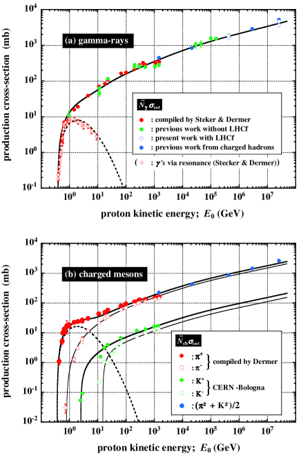
Figure 2: Total production cross sections of (a) $\gamma$-rays, $\sigma_{\rm inel}\times(\bar{N}_{\gamma}+\bar{N}_{\gamma}^{\Delta})$ and (b) charged mesons, $\sigma_{\rm inel}\times(\bar{N}_{\rm ch}+\bar{N}_{\rm ch}^{\Delta})$ as a function of the L.F. proton kinetic energy, $E_{0}$. Broken curves correspond to the production cross sections from isobaric components, and solid ones to the superposed cross sections with [pionization + isobaric] components. See Dermer [56] for data with red symbols in both (a) and (b), and Sato et al.  [1] for data with green in (a) and blue symbols in both (a) and (b), and Antinucci et al. [55] for CERN-Bologna data on K^± in (b).

References

- [1] Sato, H., Shibata, T., and Yamazaki, R. Astropart. Phys. 36, (2012) 83. (Paper I)
- [2] Adriani, O., et al. Nature 458, (2009) 607.
- [3] Adriani, O., et al. Phys. Rev. Lett., 105, (2009) 121101.
- [4] Aguilar, M., et al. (AMS Collaboration), Phys. ReV. Lett. 110, (2013) 141102.
- [5] Golden, R. L., et al., Phys. Rev. Lett. 43, (1979) 1196.
- [6] Bogomolov, F.A. et al. 1979, Proc. 16th Int. Cosmic Ray Conf., (Kyoto), 1, 1979, p. 330.
- [7] Buffington, A. et al., ApJ, 248, (1981), 1179.
- [8] Haino, S., et al., Phys. Lett. B, 545, (2004), 1135.
- [9] DuVernois, M.A., et al., ApJ, 559, (2001), 296.
- [10] Kamionski, M. and Turner, M.S., Phys. Rev., D43, (1991), 1774.
- [11] Baltz, E.A. and Edsjö, J.E., Phys. Rev., D59, (1999), 023511.
- [12] Picozza, P., Proc. of the 4th International Conference on Particle and Fundamental Physics in Space, Geneva, 5-7 Nov. 2012.
- [13] Ackermann, M. et al., arXiv:1109.0521v1 [astro-ph.HE] 2 Sep 2011.
- [14] Ting, S.C.C., Proc. of the 4th International Conference on Particle and Fundamental Physics in Space, Geneva, 5-7 Nov. 2012.
- [15] Stecker, F.W., Ap & SS, 6, (1970), 377.
- [16] Stecker, F.W., ApJ, 185, (1973), 499.
- [17] Strong, A. W., et al., ApJ, MNRAS, 182, (1978), 751.
- [18] Stephens, S.A., and Badhwar, G.D., Ap & SS, 76, (1981), 213.
- [19] Dermer, C.D., ApJ, 307, (1986), 47.
- [20] Dermer, C.D., A & A, 157, (1986), 223.
- [21] Kamae, T., et al., ApJ, 647, (2006), 692.
- [22] Neuhofer, G. et al., Phys. Lett. B, 38, (1972), 51.
- [23] Sako, T. et al., Nucl. Instrum. Methods A, (2007), 578, 146.
- [24] Lattes, C.M.G. et al., Suppl. Prog. Theor. Phys. 47, (1971), 1.
- [25] Santos, M.B.C. et al., ICR-Report-91-81-7, Univ. of Tokyo, July 1, 1981.
- [26] Adriani, O., et al., Phys. Lett. B, 703, (2011), 128.
- [27] Mase, T. et al., Nucl. Instrum. Methods A, (2012), 671, 129.
- [28] Fermi, E., Prog. Theor. Phys., 6, (1950), 4
- [29] Ciok, P. et al., Nuovo Cimento 8, (1958), 166.
- [30] Cocconi, G. et al., Phys. Rev. 111, (19589, 1699.
- [31] Niu, K. et al., Nuovo Cimento 10, (1958), 994
- [32] Peters, B., CERN 66-22, 24, June 1966.
- [33] Takagi, S., Prog. Theor. Phys., 7, (1952), 123.
- [34] Koba, J. and Takagi, S., IL NUOVO CIMENTO, X, (1958), 5.
- [35] Koshiba, M., Prog. Theor. Phys. 37, (1967), 5.
- [36] Sjostrand, T., Mrenna, S., and Skands, P., J. High Energy Phys., 05, 026, 2006.
- [37] Hayakawa, S., Gendai Butsurigaku III C, Iwanami (in Japanese), 1958.
- [38] Hayakawa, S., Cosmic Ray Physics. Wiley-Interscience, 1969.
- [39] Stecker, F.W., Cosmic Gamma Rays (NASA Scientific and Technical Information Office) NASA SP-249, 1971.
- [40] Karlsson, N., & Kamae, T., ApJ, 674, (2008), 278.
- [41] Murphy, R. J., Dermer, C. D., and Ramaty, R., ApJs, 63, (1987), 721.
- [42] Egberts, K., et al., Proc. 33rd Int. Cosmic Ray Conf., (Rio de Janeiro), 2013, to be published.
- [43] Actis, M. et al., The CTA Consortium 2010, arXiv:1008.3703v3 [astro-ph.IM] 1 1 Apr 2012.
- [44] Cavallo, G., and Gould, R.J., Nuovo Cimento, 2B, (1971), 77.
- [45] Gaisser, T.K., and Schaefer, R.K., ApJ, 394, (1992), 174.
- [46] Shibata, T., Honda, N., and Watanabe, J., Astropart. Phys., 27, (2007), 411. (Paper IV)
- [47] Mori, M., arXiv:0903.3260v2 [astro-ph.HE] 27 Apr 2009.
- [48] Panov, A. D. et al. (ATIC), Adv. Space Res., 37, (2006), 1944.
- [49] Ave, M. et al. (TRACERR), ApJ, 678, (2008), 262.
- [50] Ahn, et al. (CREAM), ApJ, 707, (2009), 593.
- [51] Commins, E., 1973, Weak Interactions (New York: McGraw-Hill)
- [52] Orth, C.D. and Buffington, A., ApJ, 206, (1976), 312
- [53] Barr, S., Gaisser, T.K., Tilav, S. and Lipari, P., Phys. Lett. 214, (1988), 147
- [54] Moskalenko, I.V. and Strong, A.W., ApJ, 493, (1998), 694
- [55] Antinucci, M., et al., CERN-Bologna ISR Collaboration, Nuovo Cimento Lett. 6, (1973), 121
- [56] Dermer, C. D., Strong, A. W., Orlando, E., Tibaldo, L., and for the Fermi Collaboration 2013, arXiv:1307.0497.
- [57] Adriani, O., et al. 2012, arXiv:1207.7183v1 [hep-ex] 31 Jul 2012.
- [58] Bergström, L., Ullio, P. and Buckley, J. H., Astropart. Phys. 9, (1998) 137.
- [59] Baltz, E.A. and Edsjö, J.E., 1999, Phys. Rev., D59, 023511.
- [60] Hisano, J., Kawasaki, M., Kohri, K., and Nakayama, K. 2009a, Phys. Rev., D79, 063514.
- [61] Hisano, J., Kawasaki, M., Kohri, K., and Nakayama, K. 2009b, Phys. Rev., D79, 083522.