A Peer-based Model of Fat-tailed Outcomes

Abstract

It is well known that the distribution of returns from various financial instruments are leptokurtic, meaning that the distributions have “fatter tails” than a Normal distribution, and have skew toward zero. This paper presents a graceful micro-level explanation for such fat-tailed outcomes, using agents whose private valuations have Normally-distributed errors, but whose utility function includes a term for the percentage of others who also buy.

1 Introduction

Many researchers have pointed out that day-to-day returns on equities have “fat tails,” in the sense that extreme events happen much more frequently than would be predicted by a Normal distribution, and have skew toward zero, meaning that extreme negative returns are more likely than extreme positive returns. This has been re-verified by many of the sources listed below. The fat tails of actual equity return distributions is far from academic trivia: if extreme events are more likely than predicted by a Normal distribution, models based on Normally-distributed returns can systematically under-predict risk.

Here, I present an explanation for the non-Normality of equity returns using a micro-level model where agents observe and emulate the behavior of others. There are several reasons for rational agents to take note of the actions of other rational agents; the model here is agnostic as to which best describes real-world agents, but given some motivation to emulate others, I show that the wider-than-Normal distribution of equity returns follows.

From the tulip bubble of 1637 to the housing bubble of 2007, herding behavior has been used to explain extreme market movements (Mackay, 1841; Schiller, 2008). Most of the literature discussed below focuses on models where the herd almost always leads itself to an extreme outcome, where goods are blockbusters or flops. Typically, agents in these models have private information or preferences that are easily drowned out by observing the behavior of others (and in some cases they have no private information at all). Conversely, the model here shows that when agents have an evaluation strategy that is a mix of both private preferences and public actions or information, then outcome distributions look much like that of day-to-day equity returns: they may have kurtosis and skew that are arbitrarily large, but they remain unimodal. As the individual utility function is adjusted so that private information is of little value, the model outcomes replicate the blockbusters, flops, and market bifurcations in the literature.

Section 2 will give a quick overview of the mostly empirical literature that has demonstrated that equity returns are fat-tailed, and that equity traders (and those who advise equity traders) demonstrate emulative behavior. Epstein and Axtell (1996, p 20, emphasis in original.) wrote “Perhaps one day people will interpret the question ‘Can you explain it?’ as asking ‘Can you grow it?”’ Section 3 will demonstrate that once we take emulative behavior as given, it is easy to grow fat-tailed outcomes. Section 4 concludes, pointing out that, because situations where outcomes are fat-tailed but not entirely off the charts are common, we may be able to use emulative preferences to explain more than they have been used for in the past.

2 Literature

This section gives an overview of two threads of the economics literature that do not quite meet. The first is an overview of the existing literature on the distribution of equity returns; the second is a survey of the situations posited in the finance literature where individuals gain utility from emulating others.

2.1 Fitting non-Normal distributions

The second central moment, also known as the variance, is defined as:

$$\mu_{2}=\sigma^{2}=\int_{-\infty}^{\infty}(x-\mu)^{2}f(x)dx,$$

where $x\in{\mathbb{R}}$ is a random variable, $f(x)$ is the probability distribution function (PDF) on $x$, and $\mu$ is the mean of $x$ $\left(\int_{-\infty}^{\infty}xf(x)dx\right)$.

One could similarly define the third and fourth central moments:

$$\mu_{3} = \int_{-\infty}^{\infty}(x-\mu)^{3}f(x)dx,\hbox{ and}$$

$$\mu_{4} = \int_{-\infty}^{\infty}(x-\mu)^{4}f(x)dx.$$

Depending on the author, the skew is sometimes the third central moment, ${\cal{S}}\equiv\mu_{3}$, and sometimes ${\cal{S}}\equiv\mu_{3}/\sigma^{3}$. The kurtosis may be $\kappa\equiv\mu_{4}$, $\kappa\equiv\mu_{4}/\sigma^{4}$, or $\kappa\equiv\mu_{4}/\sigma^{4}-3$. In this paper, I will use

$${\cal{S}} \equiv \mu_{3}\hbox{, and}$$

$$\kappa \equiv \mu_{4}/\sigma^{4}.$$

I will refer to $\kappa$ as normalized kurtosis to remind the reader that it is divided by variance squared.

The more elaborate normalizations make it easy to compare these moments to a Normal distribution, because for a Normal distribution with mean $\mu$ and standard deviation $\sigma$, $\mu_{4}/\sigma^{4}=3$. A Normal distribution is symmetric and therefore has zero skew (whether normalized or not). One can use these facts to check empirical distributions for deviations from the Normal.

Fama (1965) ran such a test on equity returns, and found that they were leptokurtic, meaning that $\mu_{4}\gg 3\sigma^{4}$, and were skewed. However, he is not the first to notice these features—Mandelbrot (1963, footnote 3) traces awareness of the non-Normality of return distributions as far back as 1915. Many of the papers cited in the following few paragraphs reproduce the results using their own data sets. Bakshi et al. (2003) gathered data on several index and equity returns, and (with few exceptions) found a skew toward zero (i.e., negative skew, meaning that extreme downward events are more likely than extreme upward events).

Most of the explanations for the deviation from the Normal have focused on finding a closed-form PDF that better fits the data. Mandelbrot (1963) showed that a stable Paretian (aka symmetric-stable) distribution fit better than the Normal. Blattberg and Gonedes (1974) showed that a renormalized Student’s $t$ distribution fit better than a symmetric-stable distribution. Kon (1984) found that a mixture of Normal distributions fit better than a Student’s $t$. The mixture model produces an output distribution by summing a first Normal distribution, ${\cal N}(\mu_{1}$, $\sigma_{1})$, with an independent second Normal distribution, ${\cal N}(\mu_{2}$, $\sigma_{2})$. Depending on the values of the five input parameters (two means, two standard deviations, and a mixing parameter), the distribution produced by summing the two can take on a wide range of mean, standard deviation, skew, and kurtosis.

The mixture model raises a few critiques. Kon found that the sum of two distributions satisfactorily matches only about half of the equity return distributions he tests. Others require as many as four input distributions—and thus eleven input parameters—to explain the four moments of the distribution to be matched. Barbieria et al. (2010, pp 1095–96) tested a set of four broad equity indices (MSCI’s USA, Europe, UK, and Japan indices) against a comparable model claiming Normality with variances changing over time, and rejected the model for all four indices.

As with all of the distribution models, the use of a sum of several distributions raises the question of how the given distributions go beyond being a good fit to being a valid explanation of market behavior. After all, one could fit a Fourier sequence to a data series to arbitrary precision, but it is not necessarily an explanation of market behavior. This brings us to the second thread of the literature, covering the micro-level behavior of market actors.

2.2 Emulation

The literature provides many rational motivations for emulating others, variously termed herding, information cascades, network effects, peer effects, spillovers—not to mention simple questions of fashion. This section provides a sample of some of the theoretical results for such models, and a discussion of herding in the finance context. None of these models were written with the stated intention of describing an observed leptokurtic distribution, but this section will calculate the kurtosis of the output distributions implied by some of these models to see how they fare.

The restaurant problem

Among the most common of the models where agents emulate others are the herding or information cascade models, e.g. Banerjee (1992) or Bikhchandani et al. (1992). In these models, agents use the prior choices of other agents as information when making decisions.

A sequence of agents chooses to eat at restaurant $A$ or $B$. The first will use its private information to choose. The second will use its private information, plus the information revealed by the observable choice made by the first agent. The third agent will add to its private information the information provided by observing where the first two entrants are eating. Thus, if the first two agents are eating at restaurant $A$, the third may ignore a preference for restaurant $B$ and eat at $A$. Once the preponderance of prior choices leans toward restaurant $A$, we can expect that all future arrivals will choose it as well. The next day, both restaurants start off empty again, and early arrivals in the sequence might have private information that restaurant $B$ is better, so subsequent arrivals would all go to restaurant $B$.

Network externalities are a property of goods where consumption by others increases the utility of the good, such as a social networking web site whose utility depends on how many others are also subscribed, computer equipment that needs to interoperate with others’ equipment, or coordination problems like the choice of whether to drive on the right or left side of the road. The typical analysis (e.g., that of Choi (1997)) matches that of the restaurant problem.

Both the information and the direct utility stories can be shown to produce a bifurcated distribution of results with probability one: over many days, restaurant $A$ will show either about 0% attendance or about 100% attendance every day. Many goods show such a blockbuster/flop dichotomy, such as movies (de Vaney and Walls, 1996).

But for our purposes, a sharply bimodal distribution is not desirable. First, one would be hard-pressed to find an equity whose returns are truly bimodal. More importantly, such a bifurcated outcome distribution is typically platykurtic, the opposite of the leptokurtosis we seek. Consider an ideal bimodal distribution with density $r\in(0,1)$ at $a$ and density $1-r$ at $b$ (for any values of $a,b\in{\mathbb{R}}$, $a\neq b$). The distribution has normalized kurtosis equal to

$$\frac{1}{r-r^{2}}-3.$$

For a symmetric distribution, $r=0.5$, the normalized kurtosis is one, and it remains less than three for any $r\in(.211,.789)$. Thus, a model that predicts a bifurcated distribution can only show a large fourth moment if the distribution is lopsided, which is not sustainable for equity returns.

Distribution models

Brock and Durlauf (2001) specify a model similar to the one presented here. In the first round, a prior percentage of actors is given, and people act iff that percentage would be large enough to give them a positive utility from acting. In subsequent rounds, individuals use the percentage of people who chose to act in the prior round to decide whether to act or not.

The specific details of Brock and Durlauf’s assumptions lead to two possible outcomes. One is a bifurcation, much like the outcomes for the restaurant problem models above. The other, due to the specific form of the assumptions, is that the output distribution is the input distribution transformed via the hyperbolic tangent. The $\tanh$ transformation reduces the normalized kurtosis, and is therefore inappropriate for deriving leptokurtic equity returns.

Glaeser et al. (1996) point out that the more people emulate others, the more likely are extreme outcomes, which they measure via “excess variance.” They do this via a Binomial model: if being the victim of a crime is a draw from a Bernoulli trial with probability $p$, then the mean of $n$ such trials is $np$, and the variance is $np(1-p)$. Thus, given $n$ and the sample mean (or equivalently, $n$ and $p$) we can solve for the expected variance, and if the observed variance is significantly greater, then we can reject the hypothesis of independent Bernoulli trials. However, this process says nothing about whether the observed victimization rates are Normally distributed or not: excess variance is not excess kurtosis or skew.

Finance

Within the theoretical finance literature, papers abound regarding herding behavior (e.g., Grossman (1976, 1981), Radner (1979), Choi (1997), Minehart and Scotchmer (1999)), although they concern themselves not with explaining herding, but with the information aggregation issues entailed by herding. Many stories regarding the emulation of others apply to the situation of the rational, self-interested manager of an asset portfolio:

• Pricing is partly based on the value of the underlying asset and partly on what others are willing to pay for the asset. At the extreme, people will buy a stock which pays zero dividends only if they are confident that there are other people who will also buy the stock; as more people are willing to buy, the value of the stock to any individual rises.

• It has long been a lament of the fund manager that if the herd does badly but he breaks even, he sees little benefit; but if the herd does well and he breaks even, then he gets fired. Therefore, behaving like others may explicitly appear in a risk-averse fund manager’s utility function.

• Since an undercapitalized company is likely to fail, the success of a public offering may depend on how well-subscribed it is, providing another justification for putting the behavior of others in the fund manager’s utility function.

• If a large number of banks take simultaneous large losses, then they may be bailed out; since a bail-out is unlikely if only one bank takes a loss, this may also serve as an incentive for financiers to take risks together.

• Simply following the herd: “[…] elements such as fashion and sense of honour affected the banks’ decision to take part in a syndicated loan. Banks are certainly not insensitive to prevailing trends, and if it is ‘the in thing’ to take part in syndicated loans[…], people sometimes consent too readily.” (Jepma et al., 1996, p 337)

The model of this paper is a reduced form model which simply assumes that a financier’s expected utility from an action is increasing with the percentage of other people acting. I make no effort to explain which of the above motivations are present at any time, but assert that given these effects, the model below is applicable.

Empirical studies of analyst recommendations find that they do indeed herd. For example, Graham (1999) finds evidence of herding among investment newsletter recommendations, and finds that the more reputable ones are more likely to herd. Meanwhile, Hong et al. (2000) finds evidence of herding among investment analysts, and finds that inexperienced analysts are “more likely to be terminated for bold forecasts that deviate from consensus,” and therefore less reputable analysts are more likely to herd. Welch (2000) finds that an analyst recommendation has a strong impact on the next two recommendations for the same security by other analysts, and that this effect is uncorrelated with whether the recommendations prove to be correct or not. Although these papers disagree in the details, they all find empirical evidence that analysts are inclined to behave like other analysts (and therefore the people who listen to analysts are likely to also behave alike), so the model below is apropos.

3 The model

One run of the model below finds an output equilibrium demand given an input distribution of individual preferences. Repeating a single run thousands of times gives a distribution of equilibrium outcomes, which will have large kurtosis and skew under certain conditions.

One run of the model consists of a plurality of agents (the simulations below use 10,000), each privately deciding whether to purchase a good. Each has an individual taste for consuming, $t\in{\mathbb{R}}$, where $t\sim{\cal N}(\epsilon,1)$ and $\epsilon$ is a small non-negative offset, fixed at zero or 0.05 in the simulations to follow.

Let the proportion of the population consuming be $k\in[0,1]$, and let the desire to emulate others be represented by a coefficient $\alpha\in[0,\infty)$. Then the utility from consuming is

$$U_{c}=t+\alpha k.$$ (1)

The utility from not consuming is

$$U_{nc}=\alpha(1-k).$$ (2)

That is, agents who do not consume get utility from emulating the $1-k$ agents who also do not consume, but have a taste for non-consumption normalized to zero. One can show that this normalization is without loss of generality. Agents consume iff $U_{c}>U_{nc}$.

A Bayesian Nash equilibrium is a set of acting agents, comprising the proportion $k_{a}$ percent of the population, where all acting agents have $U_{c}>U_{nc}$ given $k_{a}$ percent acting, and all agents outside the acting set have $U_{c}\leq U_{nc}$ given $k_{a}$ percent acting.

It can be shown that, given the assumptions here, the game has a cutoff-type equilibrium, where there is a cutoff value $T$ such that every agent with private tastes greater than $T$ acts and every agent with $t\leq T$ does not act. An agent with private taste $t$ equal to the cutoff $T$ will have $U_{c}=U_{nc}$.

One could embed this model of the distribution of demand into a larger model, such as a simple supply-demand model where supply remains fixed and demand shifts as per the model here, and prices thus vary with demand. To maintain focus on the core concept, this paper will cover only the core model describing the distribution of $\hat{k}$.

3.1 Implementation

Recall the restaurant problem, where we measured the turnout to restaurant $A$ every day for a few weeks or months. Each day gave us another draw of diners from the population, and it was the aggregate of turnouts over several days that added up to the bimodal distribution. Similarly, the literature on equities did not claim that if we surveyed willingness to pay by all members of the market at some instant in time, the distribution would be leptokurtic; rather, the claim is that every day there is a new distribution of willingness to pay, which produces a single outcome for the day, and tallying those outcomes over time generates a leptokurtic distribution. This model draws a sample distribution (which one could think of as today’s market, and which will be close to a Normal distribution), finds the equilibrium value $\hat{k}$, and then repeats until there are enough samples of $\hat{k}$ that we can estimate the moments of $\hat{k}$’s distribution.

We must first solve for the equilibrium percent acting for a single run. Briefly switching from the equilibrium percent acting $k$ to the equilibrium cutoff taste $T$, one can find the equilibrium for a single distribution by finding the value of $T$ such that an agent with that value is indifferent between action and inaction, given that the cutoff is at that value (that is, $U_{c}$ in Equation 1 equals $U_{nc}$ in Equation 2). Write the proportion not acting given cutoff $T$ as $\hbox{CDF}(T)$ (i.e. the cumulative distribution function of the empirical distribution of tastes up to the cutoff $T$); then any value of $T$ that satisfies

$$T=\alpha(1-2\hbox{CDF}(T))$$ (3)

is an equilibrium.

There are typically no closed-form solutions for $T$, so the work will require a numeric search.

I use an agent-based simulation to organize the draws. For each step, the simulation draws 10,000 agents from the fixed distribution, then the simulation algorithm solves for equilibrium via tatônnement, as detailed below. The equilibrium reached via market simulation is a Bayesian Nash equilibrium as in Equation 3. There are other search strategies for finding the equilibrium given the draws of $t$, but the agent-based model has the advantages of always finding the equilibrium and providing a realistic story of what happens in the market.

Repeating the process for thousands of draws from the fixed distribution, starting each simulation with a new set of random draws of tastes $t$ from the same distribution, will produce a distribution of the statistics $\hat{T}$ and $\hat{k}$, including multiple modes when there are multiple equilibria.

The algorithm for a single run of the simulation is displayed in Figure 1. In each step, agents consume or do not based on the value of $k$ from the last step, and the process repeats until the value of $k$ no longer changes. The output of the process is the equilibrium value of $\hat{T}$ and the equilibrium percent acting $\hat{k}$.

With a sufficiently large number of runs (in the simulations here, 20,000), it is possible to calculate the moments ${\cal{S}}(\hat{k})$ and $\kappa(\hat{k})$.

–Fix $N$ and $\epsilon$.
–Generate a new population of agents:
Hey.–Set the initial value of $k=\frac{1}{2}$.
Hey.–For each agent:
Hey.Hey.–Draw a taste $t$ from a ${\cal N}(\epsilon,1)$ distribution.
–While $k$ this period is not equal to $k$ last period:
Hey.–For each agent:
Hey.Hey.–Consume iff $U_{k}\geq U_{nk}$.
Hey.–Recalculate $k$.
–Record the equilibrium percent acting $k$.

Figure 1: The algorithm for finding the equilibrium level of consumption for one run.

The code itself is a short script written in C using the open source Apophenia library (Klemens, 2008), and is available upon request.

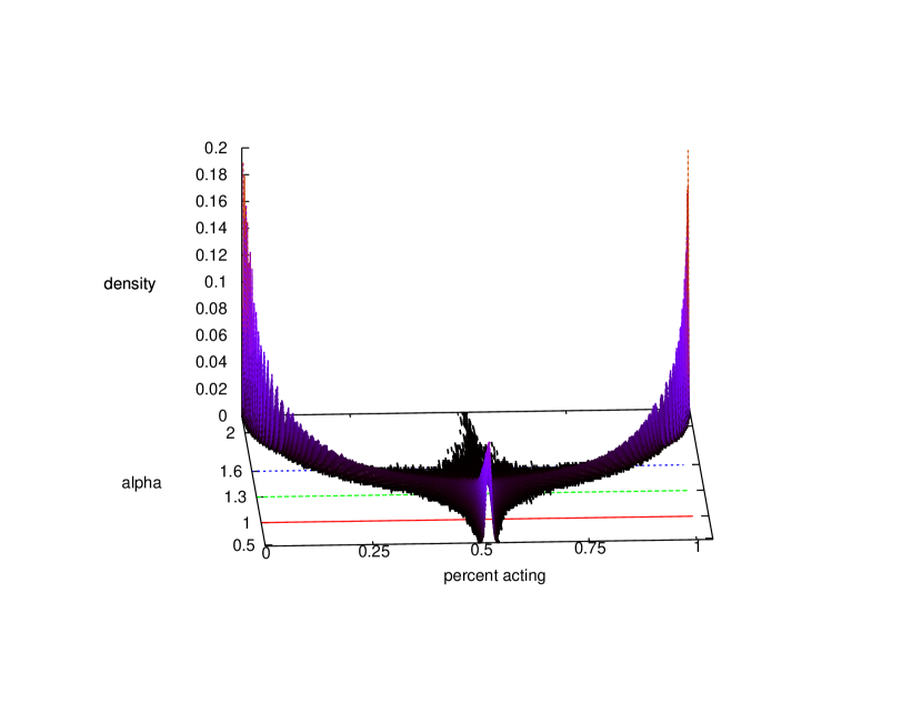
Figure 2: Above, three distributions of the equilibrium percent acting $k$, for 20,000 runs with $\alpha$ equal to 1 (unimodal), 1.3 (bimodal with modes near 0.3 and 0.7), and 1.6 (bimodal with modes near 0.1 and 0.9). Below, a full sequence of such distributions, for $\alpha=0.5$ in front up to $\alpha=2$ at the back. Vertical axis is the percent of runs (out of 20,000 per $\alpha$) whose equilibrium is in the given histogram bin. The three slices in the 2-D plot are indicated by a line on the floor of the 3-D plot.

Figure 3: The normalized kurtosis reveals the narrow range of transition from Normal-type distribution ($\kappa/\sigma^{4}=3$) to bimodal-type distribution ($\kappa/\sigma^{4}=1$).

3.2 Results

It is instructive to begin with the symmetric case, where $\epsilon=0$, so agents’ private tastes are drawn from a ${\cal N}(0,1)$ distribution.

Figure 2 shows a sequence of distributions of the equilibrium percent acting $k$, from the distribution given $\alpha=1$ up to the distribution for $\alpha=2.5$, with distributions for three specific values of $\alpha$ highlighted. Small values of $\alpha$ (where utility is mostly private valuation) result in a Normal output distribution of prices, while large values of $\alpha$ (where utility is mostly public) give a coordination-game style bifurcation.

As $\alpha$ goes from the Normal range to the bifurcated range, there is a small range of $\alpha$ where the transition occurs, and the distribution is neither fully bifurcated nor Normal.

At large $\alpha$, the value of $k$ between the sink that sends the simulation to the lower equilibrium and the sink that sends the simulation to the higher equilibrium (near 0.5) is an unstable equilibrium; in theory it occurs with probability zero, but in a finite simulation it occurs with small probability. Below, we will see that these distributions with a small middle mode behave like a bifurcated distribution, so I will refer to them as such.

The small transition range is especially clear when we look at the normalized kurtosis of each $\alpha$’s distribution, which is not at all a uniform shift. As in Figure 3, the normalized kurtosis is consistently three for small values of $\alpha$ (as for a Normal distribution), is consistently one for large values of $\alpha$ (as for a symmetric bimodal distribution), and has a quick period of transition between $\alpha\approx 1$ and $\alpha\approx 1.4$.

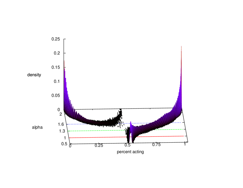
Figure 4: Two views of the $\alpha$-to-cutoff-frequency relation. PDFs of cutoffs for three given levels of $\alpha$ (1=unimodal near center, 1.3=unimodal to right, 1.6=bimodal) are displayed in 2-D form at top. At bottom is a series of PDFs for a range of values of $\alpha$ from $\alpha=0.5$ at front to $\alpha=2$ at rear.

Figure 5: The relationship between $n$ (on the horizontal axis) and $\kappa/\sigma^{4}$ (on the vertical axis, top) or ${\cal{S}}/\sigma^{3}$ (on the vertical axis, bottom).

Figure 4 shows the sequence of distributions where $\epsilon=0.05$. For $\alpha\approx 0$, the distribution is roughly equivalent to the $\epsilon=0$ situation but shifted upward slightly; for $\alpha\approx 2$ and above, where the outcome distribution is bifurcated, the slight shift in the distribution’s center causes positive outcomes to be more likely than negative outcomes.

However, between these two outcomes lies a range of $\alpha$ where the $\epsilon=0$ case would have led to a bifurcation, but the lower tail of the distribution is suppressed because the nobody-acts equilibrium is not feasible. In this range, we have an asymmetric but unimodal distribution.

Figure 5 plots normalized kurtosis for each $\alpha$’s distribution. The neighborhood of $\alpha\approx 1.3$ is again salient, because the normalized kurtosis in that range is an order of magnitude larger than three. The model’s exceptional success in generating a leptokurtic outcome makes the plot’s vertical scale rather large, so it may be difficult to discern that the kurtosis up to the peak is three, and after the peak is one, as in the $\epsilon=0$ case.

The bottom plot of Figure 5 shows that normalized skew follows the same story relative to $\alpha$ as did kurtosis: it spikes around 1.3, where the distribution of equilibrium percent acting has heavily negative skew.

Thus, given a realistic value of $\epsilon$ (i.e., anything but exactly zero), and a value of $\alpha$ that is not too small to be equivalent to the private preferences case and not too large to be equivalent to the full herding case, the distribution of outcomes is unimodal, leptokurtic, and has a negative skew.

4 Conclusion

There are several explanations for why rational agents would choose to emulate others, all of which advise that a utility function meant to describe a trader in the finance markets should include a term for the desire to emulate others.

Meanwhile, we know that equity return distributions show certain consistent deviations from the Normal distribution implied by naïve application of a Central Limit Theorem. Adding a term for the emulation of others to individual utilities produces aggregate outcome distributions that show these same deviations from Normal: extreme outcomes happen more often, and do so asymmetrically.

However, the story is not quite as simple as saying that people tend to imitate others. The type of distribution observed in equity returns appears in a middle-ground between two extreme types of utility function. With $\alpha$ small, the distribution of cutoffs is more-or-less that of a situation of purely private utility. With $\alpha$ large, the distribution follows the story of agents that simply follow the herd. But between these two situations, there is a transition range where the distribution of cutoffs has the desired characteristics of being unimodal, having large kurtosis, and skew toward zero. Thus, the model explains this type of distribution via an interplay between private and emulative utility.

This paper has shown that peer effects can generate leptokurtic outcomes under certain conditions. This creates the possibility that an observed leptokurtic distribution can be explained by peer effects. For example, Jones et al. (2003) found leptokurtic outcomes in Congressional actions such as budget allocations; I suggest in this paper that a model of Congressional representatives who emulate each other can generate such an outcome distribution. When outcomes have a blockbuster/flop bimodality, there is little doubt that peer effects are at play, but the model here shows that even more subtle outcomes, with unimodal distributions but fat tails, may also be the result of agents who gain direct or indirect utility from emulating each other.

References

- Bakshi et al. [2003] Gurdip Bakshi, Nikunj Kapadia, and Dilip Madan. Stock return characteristics, skew laws, and the differential pricing of individual equity options. The Review of Financial Studies, 16(1):101–143, Spring 2003.
- Banerjee [1992] Abhijit V Banerjee. A simple model of herd behavior. The Quarterly Journal of Economics, 107(3):797–817, Aug 1992.
- Barbieria et al. [2010] Angelo Barbieria, Vladislav Dubikovskya, Alexei Gladkevicha, Lisa R Goldberga, and Michael Y Hayesa. Central limits and financial risk. Quantitative Finance, 10(10):1091–1097, 2010.
- Bikhchandani et al. [1992] Sushil Bikhchandani, David Hirshleifer, and Ivo Welch. A theory of fads, fashion, custom, and cultural change as informational cascades. Journal of Political Economy, 100(51):992–1026, 1992.
- Blattberg and Gonedes [1974] Robert C Blattberg and Nicholas J Gonedes. A comparison of the stable and student distributions as statistical models for stock prices. The Journal of Business, 47(2):244–280, 1974.
- Brock and Durlauf [2001] William A Brock and Steven N Durlauf. Discrete choice with social interactions. Review of Economic Studies, 68:235–260, 2001.
- Choi [1997] Jay Pil Choi. Herd behavior, the “penguin effect,” and the suppression of informational diffusion: an analysis of information externalities and payoff interdependency. RAND Journal of Economics, 28(3):407–425, Autumn 1997.
- de Vaney and Walls [1996] Arthur de Vaney and W David Walls. Bose-Einstein dynamics and adaptive contracting in the motion picture industry. The Economics Journal, 47:1493–1514, November 1996.
- Epstein and Axtell [1996] Joshua M Epstein and Robert Axtell. Growing Artificial Societies: Social Science from the Bottom Up. Brookings Institution Press and MIT Press, 1996.
- Fama [1965] Eugene Fama. The behavior of stock prices. Journal of Business, 47:244–80, January 1965.
- Glaeser et al. [1996] Edward L Glaeser, Bruce Sacerdote, and Jose A Scheinkman. Crime and social interactions. The Quarterly Journal of Economics, 111(2):507–48, May 1996.
- Graham [1999] John R Graham. Herding among investment newsletters: Theory and evidence. Journal of Finance, 54(1):237–268, February 1999.
- Grossman [1981] Sanford J Grossman. An introduction to the theory of rational expectations under asymmetric information. Review of Economic Studies, 48:541–559, 1981.
- Grossman [1976] Sanford J Grossman. On the efficiency of competitive stock markets where trades have diverse information. The Journal of Finance, 31(2):573–585, May 1976.
- Hong et al. [2000] Harrison Hong, Jeffrey D Kubik, and Amit Solomon. Security analysts’ career concerns and herding of earnings forecasts. RAND Journal of Economics, 31(1):121–144, Spring 2000.
- Jepma et al. [1996] C J Jepma, H Jager, and E Kamphuis. Introduction to International Economics. Addison–Wesley, 1996.
- Jones et al. [2003] Bryan D Jones, Tracy Sulkin, and Heather A Larsen. Policy punctuations in American political institutions. American Political Science Review, 97(1):151–169, February 2003.
- Klemens [2008] Ben Klemens. Modeling with Data: Tools and Techniques for Statistical Computing. Princeton University Press, 2008.
- Kon [1984] Stanley J Kon. Models of stock returns–a comparison. The Journal of Finance, 39(1):147–165, 1984.
- Mackay [1841] Charles Mackay. Popular Delusions and the Madness of Crowds. Richard Bentley, 1841.
- Mandelbrot [1963] Benoit Mandelbrot. The variation of certain speculative prices. The Journal of Business, 36(4):394–419, 1963.
- Minehart and Scotchmer [1999] Deborah Minehart and Suzanne Scotchmer. Ex post regret and the decentralized sharing of information. Games and Economic Behavior, 27:114–131, 1999.
- Radner [1979] Roy Radner. Rational expectations equilibrium: Generic existence and the information revealed by prices. Econometrica, 47(3):655–678, May 1979.
- Schiller [2008] Robert J Schiller. How a bubble stayed under the radar. New York Times, March 2008.
- Welch [2000] Ivo Welch. Herding among security analysts. Journal of Financial Economics, 58:369–396, 2000.