Optimal Feedback Rate Sharing Strategy in Zero-Forcing MIMO Broadcast Channels

Abstract

In this paper, we consider a multiple-input multiple-output broadcast channel with limited feedback where all users share the feedback rates. Firstly, we find the optimal feedback rate sharing strategy using zero-forcing transmission scheme at the transmitter and random vector quantization at each user. We mathematically prove that equal sharing of sum feedback size among all users is the optimal strategy in the low signal-to-noise ratio (SNR) region, while allocating whole feedback size to a single user is the optimal strategy in the high SNR region. For the mid-SNR region, we propose a simple numerical method to find the optimal feedback rate sharing strategy based on our analysis and show that the equal allocation of sum feedback rate to a partial number of users is the optimal strategy. It is also shown that the proposed simple numerical method can be applicable to finding the optimal feedback rate sharing strategy when different path losses of the users are taken into account. We show that our proposed feedback rate sharing scheme can be extended to the system with stream control and is still useful for the systems with other techniques such as regularized zero-forcing and spherical cap codebook.

I Introduction

In recent years, multiple-input multiple-output (MIMO) broadcast channel (BC) systems, constructed by an access point with multiple antennas and many users, have been intensively studied [1, 2, 3]. In a MIMO BC, multiple users are simultaneously served through independent user specific multiple data streams and a multiplexing gain is attained as in point-to-point MIMO. The capacity region of the Gaussian MIMO BC was derived in [3] where dirty paper coding (DPC) [4] is known to be a capacity achieving scheme. Because DPC is hard to implement, many practical techniques have been proposed such as zero-forcing precoding (channel inversion) [5] and Tomlinson-Harashima precoding [6]. In these schemes, multiuser interference is pre-canceled at the transmitter with perfect channel state information at the transmitter (CSIT).

CSIT can be obtained by reciprocity between uplink and downlink channels in time division duplexing (TDD) systems and feedback from receivers in frequency division duplexing (FDD) systems. In FDD systems, the amount of feedback information is in general limited and hence perfect CSIT is not available. The accuracy of CSIT depends on both the type of feedback technique and the amount of feedback overhead allowed. A popular feedback architecture is a codebook approach where an index of a codeword in a predetermined codebook is fed back to the transmitter [7]. There have been many studies on the performance of codebook based multi-user MIMO systems using various transmission schemes such as zero-forcing (ZF) beamforming [8], block diagonalization (BD) [9, 10], and the unitary precoding [11].

In limited feedback environments, a key difference between MIMO BC and point-to-point MIMO is the multiplexing gain achievability [7, 8]. In point-to-point MIMO, a full multiplexing gain is achievable even with open-loop transmission. On the other hand, a full multiplexing gain cannot be achieved using a finite amount of feedback information in a MIMO BC [8]. The multiplexing gain of MIMO BC rather diminishes in the high signal-to-noise ratio (SNR) region due to imperfect orthogonalization resulting from inaccurate CSIT. To maintain the multiplexing gain, it was shown in [8, 9] that the feedback size should linearly increase with SNR (in decibel scale).

Since a large amount of feedback is a heavy burden on uplink capacity, many studies have been devoted to increasing the efficiency of limited feedback. In [12], a feedback reduction technique has been proposed using multiple antennas at the receiver. User selection in MIMO BC has been studied to reduce the amount of uplink feedback [13, 14, 15, 16, 17]. In [14], random beamforming was generalized and semi-orthogonal user selection was proposed. Also, it was shown that channel quality information as well as channel direction information are necessary to obtain both the maximum multiplexing and diversity gains. In [16], a dual-mode limited feedback system was proposed to switch between single user and multiuser transmissions. The authors in [17] investigated two partial feedback schemes for user scheduling.

In practical systems, the uplink capacity of control channels is typically limited and shared among multiple users. A sum feedback rate constraint in space division multiple access (SDMA) was considered in [18] but the amount of feedback information per user was held constant. In [19], the optimum feedback size per user and the number of feedback users were investigated under a sum feedback rate constraint assuming all users employ the same amount of feedback. Recently, strategies of feedback bit partitioning between the desired and interfering channels proposed in [20] for a cooperative multicell system. In $K$-user multiple-input-single-output (MISO) interference channel, the feedback rate control to minimize the average interference power was proposed in [21].

In MIMO BC, the effects of different amounts of feedback size among the users are studied in [22, 25, 23, 24]. In [22], the feedback rate sharing strategy has been proposed to minimize the upper bound of sum rate loss in correlated single-polarized and dual-polarized channels, respectively. The feedback rate sharing strategies in the low and high SNR regions have been proposed in terms of the correlation coefficient. The feedback rate sharing strategy to increase the sum rate was also proposed in [23] by considering users’ path losses, where the system performance was shown to be improved by changing feedback bit allocation according to the path losses. However, when the path losses are similar, the feedback rate sharing strategy in [23] is to equally share the sum feedback size regardless of SNR levels but it is not optimal in some SNR regions. Also, the effects of path losses are canceled out in the high SNR region so that equal sharing of the sum feedback size is not optimal any more. The feedback rate sharing strategy to minimize total transmission power for given users’ outage probabilities was proposed in [24].

In this paper, we provide a new analytical framework for the feedback rate sharing strategy and rigorously analyzed the effects of different amounts of feedback information among users by extending and generalizing the results of [25]. The effects of feedback rate sharing on the achievable rate are investigated in a MIMO BC with ZF beamforming at the transmitter and random vector quantization (RVQ) [26] at each user. We derive the optimal feedback rate sharing strategies according to various SNR regions. Our analytical results prove the optimal feedback rate sharing strategy in the low and the high SNR regions. The feedback rate should be equally shared among all users in the low SNR region while the whole feedback rate should be allocated to a single user in the high SNR region. For the mid-SNR region, we establish a simple numerical method for finding the optimal feedback sharing strategy based on our analytical framework. Through the proposed numerical method, we find that to equally allocate whole feedback size to a partial number of users is the optimal feedback rate sharing strategy. For the users suffering different path losses, we show that the proposed numerical method can be applicable to finding the optimal feedback rate sharing strategy. In the high SNR region, we prove that the effects of path losses are canceled out and hence the optimal feedback strategy is to allocate the whole feedback size to a single user with the highest SNR. Our proposed feedback rate sharing strategy derived from the system with ZF beamforming and RVQ is also evaluated for the systems with other techniques such as stream control, regularized ZF transmission scheme and spherical cap codebook model [27, 14]. Our numerical results show that our proposed feedback rate sharing strategy is still valid for other configurations.

The rest of this paper is organized as follows. We describe the system model and formulate the problem in Section II. The impacts of asymmetric feedback size among users are investigated in Section III. The optimal sum feedback rate sharing strategy is derived in Section IV. The numerical results are shown in Section V. Section VI concludes our paper.

II Problem Formulation

II-A System Model

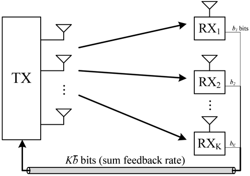
Figure 1: A system model. The sum feedback rate is shared by all users.

Our system model is depicted in Fig. 1. We consider a MIMO BC with $M$ transmit antennas and $K(=M)$ users having a single antenna. If the receiver has multiple antennas, each antenna can be considered as an independent user, or receive combining discussed in [12] can be adopted. The received signal at the user $k$ becomes

$$y_{k}=\sqrt{\gamma_{k}}\mathbf{h}_{k}^{\dagger}\mathbf{x}+n_{k},\quad k=1,\ldots,K,$$

where $\gamma_{k}$ is the path loss of the $k$th user, $\mathbf{h}_{k}\in\mathbb{C}^{M\times 1}$ is a channel vector whose entries are independent and identically distributed (i.i.d.) circularly symmetric complex Gaussian random variables with zero mean and unit variance, $\mathbf{x}\in\mathbb{C}^{M\times 1}$ is the transmit signal vector, $n_{k}$ is a complex Gaussian noise with zero mean and unit variance, and the superscript $\dagger$ denotes conjugate transposition of a vector. When $P$ is the transmit signal power, $\mathbf{x}$ satisfies that $\mathbb{E}[tr\left(\mathbf{x}\mathbf{x}^{\dagger}\right)]=P$. If users demand the same quality of service, the propagation path losses need to be pre-compensated to yield the same average SNR at the receiver in downlink. Thus, we firstly assume that the different propagation path losses for users are compensated by the transmitter, i.e., $\gamma_{1}=\gamma_{2}=\cdots=\gamma_{K}=1$. The open loop power control is also useful for preventing waste of transmit power and avoiding extra interference to other users. Then, we extend our results to different path loss scenarios in Section IV-D.

As a simple linear precoding scheme, we adopt a ZF beamforming scheme in which the data stream for each user is aligned with its precoding vector. We denote the precoding vector of the $k$th user as $\mathbf{v}_{k}$ such that $\|\mathbf{v}_{k}\|=1$ and then the transmit signal $\mathbf{x}$ becomes $\mathbf{x}=\sum_{k=1}^{K}\mathbf{v}_{k}s_{k}$, where $s_{k}$ is the data symbol for the $k$th user. We assume that the transmitter has only channel direction information (CDI) so that the feedback for power allocation can be saved. Therefore, the transmitter allocates equal power to users such that $\mathbb{E}|s_{k}|^{2}=P/M$. Also, we assume that $s_{k}$ is chosen from a Gaussian codebook and the codeword block length is sufficiently long so that it encounters all possible channel realizations for ergodicity. Obviously, power adaptation can further increase the achievable rate but the power allocation using channel quality information (CQI) is a secondary problem when the number of transmit antennas is same as the number of served users, i.e., full multiplexing [8]. In Section IV-F, we will consider the stream control where the transmitter adaptively controls multiplexing gain and the served users equally share total transmit power.

The received signal at the $k$th user using linear precoding becomes

$$y_{k}=\mathbf{h}_{k}^{\dagger}\mathbf{v}_{k}s_{k}+\sum_{i=1,i\neq k}^{K}\mathbf{h}_{k}^{\dagger}\mathbf{v}_{i}s_{i}+n_{k},\quad k=1,\ldots,K.$$ (1)

When the transmitter knows $\{\mathbf{h}_{1},\ldots,\mathbf{h}_{K}\}$ perfectly, the precoding vectors yield zero multiuser interferences, i.e., $\sum_{i\neq k}\mathbf{h}_{k}^{\dagger}\mathbf{v}_{i}s_{i}=0$; the received signal at the $k$th user becomes

$$y_{k}=\mathbf{h}_{k}^{\dagger}\mathbf{v}_{k}s_{k}+n_{k},\quad k=1,\ldots,K.$$

In most practical systems, however, the imperfect CSI is only available at the transmitter due to the limited feedback budget. The user $k$ quantizes its own channel, $\mathbf{h}_{k}$, and feeds the quantized CSI denoted by $\hat{\mathbf{h}}_{k}$ to the transmitter. Then, the transmitter finds the precoding vectors $\mathbf{v}_{1},\ldots,\mathbf{v}_{K}$ from the quantized CSI, $\hat{\mathbf{h}}_{1},\ldots,\hat{\mathbf{h}}_{K}$, instead of the perfect CSI, $\mathbf{h}_{1},\ldots,\mathbf{h}_{K}$. Because of the quantization errors, the precoding vectors obtained from the quantized CSI cannot perfectly mitigate the multiuser interference. The precoding vector cannot be exactly picked in the null space of the other users’ channel vectors; the interference term $\sum_{i\neq k}\mathbf{h}_{k}^{\dagger}\mathbf{v}_{i}s_{i}$ remains in the received signal.

At the transmitter, a quantized channel matrix defined by $\hat{\mathbf{H}}\triangleq[\hat{\mathbf{h}}_{1},\ldots,\hat{\mathbf{h}}_{K}]^{\dagger}$ is constructed with the quantized CSI fed back from the users. The $k$th normalized column vector of $\hat{\mathbf{H}}^{-1}$ becomes the precoding vector for the $k$th user, $\mathbf{v}_{k}$, where $(\cdot)^{-1}$ denotes the matrix inversion. Thus, we can decompose $\hat{\mathbf{H}}^{-1}$ as $\hat{\mathbf{H}}^{-1}=\mathbf{V}\mathbf{\Lambda}$, where $\mathbf{V}=\left[\mathbf{v}_{1},\ldots,\mathbf{v}_{K}\right]$ is a zero-forcing beamforming matrix such as $\|\mathbf{v}_{k}\|^{2}=1$, and $\mathbf{\Lambda}=\textrm{diag}(\lambda_{1},\ldots,\lambda_{K})$ is diagonal matrix whose element $\lambda_{k}\in\mathbb{R}^{+}$ is the Euclidean norm of the $k$th column of $\hat{\mathbf{H}}^{-1}$.

For the channel quantization, RVQ is considered at each user, which is widely used to analyze the effects of quantization error and asymptotically optimal as the number of antennas goes to infinity [28, 8]. Although the performance is suboptimal for a small feedback size, RVQ makes the analysis tractable and provides insightful results. Furthermore, the overall trends of RVQ generally agree with the trends of other quantization models [14].

Using $b_{k}$-bit RVQ at the $k$th user, the quantized CSI is obtained by

$$\hat{\mathbf{h}}_{k}=\underset{\mathbf{w}\in\mathcal{W}_{k}}{\arg\max}~{}~{}\cos^{2}(\angle(\mathbf{h}_{k},\mathbf{w}))=\underset{\mathbf{w}\in\mathcal{W}_{k}}{\arg\max}~{}~{}|\mathbf{h}_{k}^{\dagger}\mathbf{w}|^{2},$$

where $\mathcal{W}_{k}=\{\mathbf{w}_{k,1},\ldots,\mathbf{w}_{k,2^{b_{k}}}\}$ is a random vector codebook at the $k$th user consists of $2^{b_{k}}$ randomly chosen isotropic $M$-dimensional unit vectors. The quantization error denoted by $Z_{k}\in[0,1]$ becomes

$$Z_{k}=\underset{\mathbf{w}\in\mathcal{W}_{k}}{\min}\sin^{2}(\angle(\mathbf{h}_{k},\mathbf{w}))=\sin^{2}(\angle(\mathbf{h}_{k},\hat{\mathbf{h}}_{k}))=1-|\tilde{\mathbf{h}}_{k}^{\dagger}\hat{\mathbf{h}}_{k}|^{2},$$ (2)

where $\tilde{\mathbf{h}}_{k}=\mathbf{h}_{k}/\|\mathbf{h}_{k}\|$. For an arbitrary codeword $\mathbf{w}\in\mathcal{W}_{k}$, $|\tilde{\mathbf{h}}_{k}^{\dagger}\mathbf{w}|^{2}$ is a squared inner product of two independent random vectors isotropic in $\mathbb{C}^{M}$, so follows the beta distribution with parameters $(M-1,1)$ [8, 28]. Consequently, a quantization error using $b_{k}$-bit RVQ, $Z_{k}$, becomes the minimum of $2^{b_{k}}$ independent beta distributed random variables with parameters $(M-1,1)$. Correspondingly the complementary cumulative density function (CDF) of $Z_{k}$ is given by [28]

$$\mathrm{Pr}[Z_{k}>z]=\left(1-z^{M-1}\right)^{2^{b_{k}}}.$$ (3)

II-B Feedback Rate Sharing Strategy

We assume an average feedback size allocated for each user is $\bar{b}$ so that the total feedback rate (i.e., the sum of all individual users’ feedback rates) becomes $K\bar{b}$ bits per channel realization. Assuming the feedback rate sharing among users, each user uses $b_{k}$-bit feedback and the sum feedback rate constraint becomes $\sum_{k=1}^{K}b_{k}=K\bar{b}$. Since codebook size is typically a non-negative integer number of bits, we restrict the average feedback size, $\bar{b}$, as an positive integer, i.e., $\bar{b}\in\mathbb{Z}^{+}$. For the same reason, we assume the feedback size at the $k$th user, $b_{k}$, as a non-negative integer, i.e., $b_{k}\in\{0\}\cup\mathbb{Z}^{+}$ for $k=1,\ldots,K$,

From individual feedback rates, a feedback rate sharing strategy can be expressed by $K$-dimensional vector

$$\mathbf{b}=[b_{1},\ldots,b_{K}],$$ (4)

and the sum feedback rate constraint becomes $\|\mathbf{b}\|_{1}=K\bar{b}$ where $\|\cdot\|_{1}$ is the vector one norm.

From (1), we obtain the average sum rate as a function of transmit power, $P$, and the sum feedback rate sharing strategy, $\mathbf{b}$, denoted by $\mathcal{R}(P,\mathbf{b})$ given by

$$\mathcal{R}(P,\mathbf{b})=\sum_{k=1}^{K}\mathbb{E}\left[\log_{2}\left(1+\frac{\frac{P}{M}|\mathbf{h}_{k}^{\dagger}\mathbf{v}_{k}|^{2}}{1+\sum_{i\neq k}\frac{P}{M}|\mathbf{h}_{k}^{\dagger}\mathbf{v}_{i}|^{2}}\right)\right].$$ (5)

Thus, we solve the following problem:

$$\underset{\mathbf{b}=[b_{1},\ldots,b_{K}]}{\textrm{maximize}} \qquad\mathcal{R}(P,\mathbf{b})$$ (6)

subject to $$\qquad\sum_{k=1}^{K}b_{k}=K\bar{b},$$ (7)

$$\qquad b_{k}\in\{0\}\cup\mathbb{Z}^{+}\quad k=1,\ldots,K.$$ (8)

Note that the optimal sum feedback rate sharing strategy will be derived later and shown to be dependent on the SNR value. Therefore, the feedback bits are reallocated each time when the SNR changes. In practical scenarios, several allocation patterns can be constructed offline for typical SNR values and then the transmitter can broadcast an appropriate allocation pattern using the current SNR.

III Impacts of Asymmetric Feedback Sizes among Users

To find the optimal feedback rate sharing strategy, we first analyze the impact of asymmetric feedback sizes among the users on the sum rate. For the simplicity, we define three random variables

$$Q_{k}\triangleq\|\mathbf{h}_{k}\|^{2},\quad X_{k}\triangleq|\tilde{\mathbf{h}}_{k}^{\dagger}\mathbf{v}_{k}|^{2},\quad Y_{k}\triangleq\sum_{i\neq k}|\tilde{\mathbf{h}}_{k}^{\dagger}\mathbf{v}_{i}|^{2},$$ (9)

where $Q_{k}$ is the $k$th channel gain, $X_{k}$ is the squared inner product between the $k$th normalized channel vector and the $k$th beamforming vector, and $Y_{k}$ is the sum of the squared inner products between the $k$th normalized channel vector and the other beamforming vectors. Note that $X_{k}$ is not affected by the feedback size of the $k$th user since $\mathbf{v}_{k}$ is selected in the null space of $\{\hat{\mathbf{h}}_{i}\}_{i\neq k}$.

Using the quantization error $Z_{k}$ defined in (2), we can decompose $\tilde{\mathbf{h}}_{k}$ into $\tilde{\mathbf{h}}_{k}=\sqrt{1-Z_{k}}\hat{\mathbf{h}}_{k}+\sqrt{Z_{k}}\mathbf{e}_{k}$ where $\mathbf{e}_{k}$ is an unit vector such that $|\hat{\mathbf{h}}_{k}^{\dagger}\mathbf{e}_{k}|^{2}=0$. The random variable $Y_{k}$ becomes

$$Y_{k} =\sum_{i\neq k}\left|\left(\sqrt{1-Z_{k}}\hat{\mathbf{h}}_{k}+\sqrt{Z_{k}}\mathbf{e}_{k}\right)^{\dagger}\mathbf{v}_{i}\right|^{2}$$ (10)

$$=Z_{k}\sum_{i\neq k}|\mathbf{e}_{k}^{\dagger}\mathbf{v}_{i}|^{2}$$ (11)

$$=Z_{k}\cdot W_{k},$$ (12)

where the random variable $W_{k}\triangleq\sum_{i\neq k}|\mathbf{e}_{k}^{\dagger}\mathbf{v}_{i}|^{2}$ is the sum of the square of inner products between the quantization error vector $\mathbf{e}_{k}$ and the beamforming vectors of other users $\{\mathbf{v}_{i}\}_{i\neq k}$. The independency between $Z_{k}$ and $|\mathbf{e}^{\dagger}_{k}\mathbf{v}_{i}|^{2}$ is shown in [12] from the fact that the magnitude of the quantization error, $Z_{k}$ is independent of the direction of quantization error, $\mathbf{e}_{k}$. Thus, we can easily find that $Z_{k}$ and $W_{k}(=\sum_{i\neq k}|\mathbf{e}^{\dagger}_{k}\mathbf{v}_{i}|^{2})$ are independent. We start from the following lemma.

Lemma 1.

The random variables $Q_{k}$, $X_{k}$, $W_{k}$ and $Z_{k}$ have following properties.

1. Invariant with the feedback sizes, $b_{1},\ldots,b_{K}$, the distributions of $Q_{k}$, $X_{k}$, and $W_{k}$ are identical for all users, respectively, i.e.,

   $$f_{Q_{k}}(q)=f_{Q_{1}}(q),\quad f_{X_{k}}(x)=f_{X_{1}}(x),\quad$$

   $$f_{W_{k}}(w)=f_{W_{1}}(w),\quad k=2,\ldots,K,$$

   where $f_{Q_{k}}(q)$, $f_{X_{k}}(x)$, and $f_{W_{k}}(w)$ are the marginal PDFs of $Q_{k}$, $X_{k}$, $W_{k}$, respectively,

2. $Q_{k}$, $X_{k}$, and $W_{k}$ are independent of $Z_{k}$, respectively.

3. The joint PDF of $Q_{k}$, $X_{k}$, and $W_{k}$ are identical for all users, i.e.,

   $$f_{Q_{k},X_{k},W_{k}}(q,x,w)=f_{Q_{1},X_{1},W_{1}}(q,x,w),$$

   where $f_{Q_{k},X_{k},W_{k}}(q,x,w)$ is the joint PDF of $Q_{k}$, $X_{k}$, and $W_{k}$.

Proof.

See Appendix A. ∎

Lemma 2.

The achievable rate of the $k$th user is determined by only its own feedback size $b_{k}$ and is independent of the other users’ feedback sizes $\{b_{i}\}_{i\neq k}$.

Proof.

From Lemma 1, we can rewrite the average sum rate in (5) as

$$\mathcal{R}(P,\mathbf{b}) =\sum_{k=1}^{K}\mathbb{E}_{Q_{k},X_{k},W_{k},Z_{k}}\left[\log_{2}\left(1+\frac{\frac{P}{M}Q_{k}X_{k}}{1+\frac{P}{M}Q_{k}W_{k}Z_{k}}\right)\right]$$

$$=\sum_{k=1}^{K}\mathbb{E}_{Q_{1},X_{1},W_{1},Z_{k}}\left[\log_{2}\left(1+\frac{\frac{P}{M}Q_{1}X_{1}}{1+\frac{P}{M}Q_{1}W_{1}Z_{k}}\right)\right].$$

Thus, the achievable rate at the $k$th user is dependent on only its own feedback size because $Q_{1}$, $X_{1}$, and $W_{1}$ are not affected by the feedback size as noted in Lemma 1. Since the distribution of $Z_{k}$ is a function of $b_{k}$, the achievable rate at each user is only affected by its own feedback size. ∎

Thus, the achievable rate of the user $k$ becomes a function of transmit power $P$ and own feedback size $b_{k}$ denoted by $\mathcal{R}_{k}(P,b_{k})$ such that

$$\mathcal{R}_{k}(P,b_{k})=\mathbb{E}_{Q_{1},X_{1},W_{1},Z_{k}}\left[\log_{2}\left(1+\frac{\frac{P}{M}Q_{1}X_{1}}{1+\frac{P}{M}Q_{1}W_{1}Z_{k}}\right)\right],$$ (13)

and it satisfies that $\mathcal{R}(P,\mathbf{b})=\sum_{k=1}^{K}\mathcal{R}_{k}(P,b_{k})$.

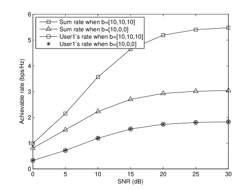
Figure 2: The sum rate and the achievable rate at the user 1 in $3\times 3$ MIMO BC. The achievable rate of user 1 is not affected by the other users’ feedback sizes, while the sum rate is increased as the feedback sizes of other users increase.

To verify Lemma 2, two feedback scenarios $\mathbf{b}_{1}=[10,10,10]$ and $\mathbf{b}_{2}=[10,0,0]$ are considered in ZF MIMO BC with $M=3$, $K=3$. In Fig. 2, the sum rate for the first scenario is much higher than that for the second scenario due to the larger amount of total feedback information. As predicted in Lemma 2, however, the achievable rate of user 1 is the same in the two scenarios.

Lemma 2 indicates that a feedback size of a user does not affect the achievable rates of the other users and only changes its own achievable rate. Under a sum feedback rate constraint, an increase of one user’s feedback size necessarily decreases other users’ feedback sizes. With more accurate $\hat{\mathbf{h}}_{k}$, the transmitter can pick the beamforming vectors of other users in more accurate null space of the user $k$. Hence, the user $k$ benefits from less interference from other users. On the other hand, the other users experience more interference since the accuracy of the users’ channel knowledge degrades under the sum feedback rate constraint. Consequently, when a user increases its own feedback size, the achievable rate of the user increases but the achievable rates of the other users decrease, and vice versa. The optimal feedback rate sharing strategy starts from this fundamental tradeoff.

IV Sum Feedback Rate Sharing Strategy

IV-A Low SNR Region

In the low SNR region, the achievable rate of the $k$th user given in (13) becomes

$$\lim_{P\to 0}\mathcal{R}_{k}(P,b_{k})$$

$$=\lim_{P\to 0}\mathbb{E}\bigg{[}\log_{2}\left(1+\frac{P}{M}Q_{1}X_{1}+\frac{P}{M}Q_{1}W_{1}Z_{k}\right)$$

$$\qquad-\log_{2}\left(1+\frac{P}{M}Q_{1}W_{1}Z_{k}\right)\bigg{]}$$

$$=\lim_{P\to 0}\mathbb{E}\bigg{[}\log_{2}\left(1+\frac{P}{M}Q_{1}X_{1}\right)+\log_{2}\left(1+\frac{\frac{P}{M}Q_{1}W_{1}Z_{k}}{1+\frac{P}{M}Q_{1}X_{1}}\right)$$

$$\qquad-\log_{2}\left(1+\frac{P}{M}Q_{1}W_{1}Z_{k}\right)\bigg{]}$$

$$\stackrel{{\scriptstyle(a)}}{{=}}\frac{1}{\ln 2}\mathbb{E}\left[\frac{P}{M}Q_{1}X_{1}\right]-\frac{1}{\ln 2}\mathbb{E}\left[\frac{\frac{P^{2}}{M^{2}}Q_{1}^{2}X_{1}W_{1}Z_{k}}{1+\frac{P}{M}Q_{1}X_{1}}\right]$$

$$\stackrel{{\scriptstyle(b)}}{{=}}\frac{1}{\ln 2}\mathbb{E}\left[\frac{P}{M}Q_{1}X_{1}\right]-\frac{1}{\ln 2}\mathbb{E}\left[\frac{\frac{P^{2}}{M^{2}}Q_{1}^{2}X_{1}W_{1}}{1+\frac{P}{M}Q_{1}X_{1}}\right]\cdot\mathbb{E}[Z_{k}],$$

where the equality $(a)$ holds because $\lim_{x\to 0}\ln(1+x)=x$, and the equality $(b)$ holds from the fact that $Z_{k}$ is independent of $Q_{k}$, $X_{k}$, and $W_{k}$ from Lemma 1. In the low SNR region, therefore, the optimization problem (6) is equivalent with the following problem:

$$\underset{\mathbf{b}=[b_{1},\ldots,b_{K}]}{\textrm{minimize}} \qquad\sum_{k=1}^{K}\mathbb{E}[Z_{k}]$$ (14)

subject to $$\qquad\eqref{eqn:constraint1},\eqref{eqn:constraint2}.$$

Definition 1 (Majorization).

For a vector $\mathbf{a}\in\mathbb{R}^{m}$, we denote by $\mathbf{a}^{\downarrow}\in\mathbb{R}^{m}$ the vector with the same components, but sorted in decreasing order. For given vectors $\mathbf{a}_{1},\mathbf{a}_{2}\in\mathbb{R}^{m}$ such that $\|\mathbf{a}_{1}\|_{1}=\|\mathbf{a}_{2}\|_{1}$, we say $\mathbf{a}_{1}$ majorizes $\mathbf{a}_{2}$ written as $\mathbf{a}_{1}\succeq\mathbf{a}_{2}$ when

$$\sum_{i=1}^{n}[\mathbf{a}_{1}^{\downarrow}]_{i} \geq\sum_{i=1}^{n}[\mathbf{a}_{2}^{\downarrow}]_{i}\qquad 1\leq n\leq m,$$ (15)

where $[\cdot]_{i}$ denotes the $i$th component of the vector.

Theorem 1 (Strategy in the Low SNR Region).

Using RVQ in the low SNR region, feedback rate sharing strategy $\mathbf{b}_{1}$ achieves higher average sum rate than feedback rate sharing strategy $\mathbf{b}_{2}$ whenever $\mathbf{b}_{1}\preceq\mathbf{b}_{2}$, i.e.,

$$\lim_{P\to 0}\mathcal{R}(P,\mathbf{b}_{1})\geq\lim_{P\to 0}\mathcal{R}(P,\mathbf{b}_{2})\quad\textrm{for all}\quad\mathbf{b}_{1}\preceq\mathbf{b}_{2}.$$ (16)

Proof.

See Appendix B. ∎

Corollary 1.

In the low SNR region, when the sum feedback rates is $K\bar{b}$ (i.e., $\sum b_{k}=K\bar{b}$), the optimal feedback rate sharing strategy is to allocate the same amount of feedback ($b_{k}=\bar{b}$) to all users while the worst strategy is to allocate whole feedback amount $K\bar{b}$ to a single user.

Proof.

All possible feedback sharing strategies $\mathbf{b}$ ($\|\mathbf{b}\|_{1}=K\bar{b}$) satisfy that

$$[\bar{b},\ldots,\bar{b}]\preceq\mathbf{b}\preceq[K\bar{b},0,\ldots,0].$$ (17)

Thus, the optimal feedback sharing strategy in low SNR region is to allocate the same feedback size to all users while the worst strategy is to allocate the whole feedback size to a single user. ∎

IV-B High SNR Region

With fixed feedback size in the high SNR region, the sum rate of a MIMO BC saturates and cannot achieve the full multiplexing gain [8]. This is because the remaining interference caused by the quantization error increases with SNR so that the SINR is saturated in the high SNR region.

For ease of explanation, we decompose the achievable rate at user $k$ into an increasing term and a decreasing term denoted by $\mathcal{R}_{k}^{+}(P,b_{k})$ and $\mathcal{R}_{k}^{-}(P,b_{k})$, respectively, given by

$$\mathcal{R}_{k}^{+}(P,b_{k}) =\mathbb{E}\left[\log_{2}\left(1+\frac{P}{M}Q_{1}X_{1}+\frac{P}{M}Q_{1}W_{1}Z_{k}\right)\right]$$

$$\mathcal{R}_{k}^{-}(P,b_{k}) =\mathbb{E}\left[\log_{2}\left(1+\frac{P}{M}Q_{1}W_{1}Z_{k}\right)\right],$$

so that $\mathcal{R}_{k}(P,b_{k})=\mathcal{R}_{k}^{+}(P,b_{k})-\mathcal{R}_{k}^{-}(P,b_{k})$. Similarly, we can express the average sum rate into two parts as $\mathcal{R}(P,\mathbf{b})=\mathcal{R}^{+}(P,\mathbf{b})-\mathcal{R}^{-}(P,\mathbf{b})$ where $\mathcal{R}^{+}(P,\mathbf{b})=\sum_{k=1}^{K}\mathcal{R}_{k}^{+}(P,b_{k})$ and $\mathcal{R}^{-}(P,\mathbf{b})=\sum_{k=1}^{K}\mathcal{R}_{k}^{-}(P,b_{k})$.

In the high SNR region, the increasing term of the $k$th user’s achievable rate, $\mathcal{R}_{k}^{+}(P,b_{k})$, becomes

$$\lim_{P\to\infty}\mathcal{R}_{k}^{+}(P,b_{k})=\mathbb{E}\left[\log_{2}\left(\tfrac{P}{M}Q_{1}\right)\right]+\mathbb{E}\left[\log_{2}\left(X_{1}+W_{1}Z_{k}\right)\right],$$

where the second term on the right hand side of the equality is only affected by the quantization error, $Z_{k}$. For the quantization error $Z_{k}\in[0,1]$, the range of $\log_{2}\left(X_{1}+W_{1}Z_{k}\right)$ becomes $\log_{2}\left(X_{1}+W_{1}Z_{k}\right)\in[\log_{2}\left(X_{1}\right),\log_{2}\left(X_{1}+W_{1}\right)]$. In the high SNR region, on the other hand, the decreasing term of the $k$th user’s achievable rate, $\mathcal{R}_{k}^{-}(P,b_{k})$, becomes

$$\lim_{P\to\infty}\mathcal{R}_{k}^{-}(P,b_{k})=\mathbb{E}\left[\log_{2}\left(\tfrac{P}{M}Q_{1}W_{1}\right)\right]+\mathbb{E}\left[\log_{2}\left(Z_{k}\right)\right],$$

where the quantization error affects $\mathbb{E}\left[\log_{2}\left(Z_{k}\right)\right]$ only. For the quantization error $Z_{k}\in[0,1]$, we can find $\log_{2}\left(Z_{k}\right)\in(-\infty,0]$. However, note that $\log_{2}\left(\frac{P}{M}Q_{1}W_{1}\right)\gg-\log_{2}Z_{k}$ when $P\to\infty$ although $\log_{2}\left(Z_{k}\right)\in(-\infty,0]$. These facts implicate that in the high SNR region the quantization error, $Z_{k}$, only dependent on the feedback size, highly affects the rate decreasing term $\mathcal{R}_{k}^{-}(P,b_{k})$ and thus the achievable rate at each user is dominated by the rate decreasing term. Therefore, the feedback rate sharing strategy in the high SNR region should be focused on minimizing the rate decreasing term. The average sum rate decreasing term, $\mathcal{R}^{-}(P,\mathbf{b})$, becomes

$$\lim_{P\to\infty}\mathcal{R}^{-}(P,\mathbf{b}) =M\mathbb{E}\left[\log_{2}\left(\frac{P}{M}Q_{1}W_{1}\right)\right]+\sum_{k=1}^{K}\mathbb{E}\left[\log_{2}Z_{k}\right].$$

Hence, as an alternative of (6) in the high SNR region, we solve the optimization problem to minimize $\mathcal{R}^{-}(P,\mathbf{b})$ equivalent with the following problem:

$$\underset{\mathbf{b}=[b_{1},\ldots,b_{K}]}{\textrm{minimize}} \qquad\sum_{k=1}^{K}\mathbb{E}[\log_{2}Z_{k}]$$ (18)

subject to $$\qquad\eqref{eqn:constraint1},\eqref{eqn:constraint2}.$$

Theorem 2 (Strategy in the High SNR Region).

Using RVQ in the high SNR region, feedback rate sharing strategy $\mathbf{b}_{1}$ achieves higher average sum rate than feedback rate sharing strategy $\mathbf{b}_{2}$ whenever $\mathbf{b}_{1}\succeq\mathbf{b}_{2}$, i.e.,

$$\lim_{P\to\infty}\mathcal{R}(P,\mathbf{b}_{1})\geq\lim_{P\to\infty}\mathcal{R}(P,\mathbf{b}_{2})\quad\textrm{for all}\quad\mathbf{b}_{1}\succeq\mathbf{b}_{2}.$$ (19)

Proof.

See Appendix C. ∎

Corollary 2.

In the high SNR region, when the total amount of feedback information from all users is fixed (i.e., $\sum b_{k}=K\bar{b}$), the optimal feedback rate sharing strategy is to allocate whole feedback amount $K\bar{b}$ to a single user while the worst strategy is to allocate the same amount of feedback ($b_{k}=\bar{b}$) to all users.

Proof.

As stated in the proof of Corollary 1, any feedback rate sharing strategy, $\mathbf{b}$, satisfies that

$$[\bar{b},\ldots,\bar{b}]\preceq\mathbf{b}\preceq[K\bar{b},0,\ldots,0].$$ (20)

Thus, the optimal feedback rate strategy in the high SNR region is to allocate the whole feedback size to a single user while the worst strategy is to allocate the same feedback size to each user. ∎

IV-C Intermediate SNR Region

In Theorem 1 and Theorem 2, the optimal feedback rate sharing strategies in the asymptotic SNR regions are derived. In the practical SNR region, the optimal strategy can easily be found by a numerical method owing to Lemma 2 that the achievable rate of each user only depends on its own feedback size. We first compute the achievable rates of each user for various feedback bits $b_{k}=0,\ldots,K\bar{b}$, respectively. Using the computed numerical values, we select the best feedback rate sharing strategy for each SNR that maximizes the total sum rate among all possible strategies. For example, when total feedback size is 16bits, the conventional exhaustive search needs to search the optimal strategy among all possible 64 strategies. On the other hand, in our proposed numerical method, it is enough to consider only five strategies – $[0,0,0,0]$, $[1,2,3,4]$, $[5,6,7,8]$, $[9,10,11,12]$, $[13,14,15,16]$ – because the achievable rate for other strategies can be easily obtained from Lemma 2. Denoting the set of all possible strategies by $\mathcal{B}$, the procedure to find the optimal feedback strategy is described in Algorithm 1. The complexity of the procedure will be analyzed in Section IV-E.

Algorithm 1 Procedure to find Feedback Rate Sharing Strategy

1:Initialization: randomly choose $\mathbf{b}\in\mathcal{B}$

2:for all $\mathbf{b}^{\prime}\in\mathcal{B}$ do

3:     if $\sum\mathcal{R}_{k}(\gamma_{k}P,[\mathbf{b}^{\prime}]_{k})>\sum\mathcal{R}_{k}(\gamma_{k}P,[\mathbf{b}]_{k})$ then

4:         $\mathbf{b}=\mathbf{b}^{\prime}$;

5:     end if

6:end for

7:Output: the optimal feedback strategy $\mathbf{b}$

Observation 1.

The optimal feedback rate sharing strategy is to allocate the same amount of feedback to the optimal number of users at given SNR.

TABLE I: The optimal feedback rate sharing strategy for a $4\times 4$ MIMO BC

2 streams		3 streams		4 streams
SNR(dB)	$\mathbf{b}^{\downarrow}$	SNR	$\mathbf{b}^{\downarrow}$	SNR	$\mathbf{b}^{\downarrow}$
0$\sim$27	[12,12]	0$\sim$12	[8,8,8]	0$\sim$7	[6,6,6,6]
28$\sim$	[24, 0]	13$\sim$23	[12,12,0]	8$\sim$11	[8,8,8,0]
		24$\sim$	[24,0,0]	12$\sim$20	[12,12,0,0]
				21$\sim$	[24,0,0,0]

Example 1.

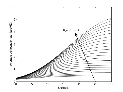
Figure 3: Achievable rate of a single user using $b_{k}$ feedback bits in a $4\times 4$ MIMO BC.

For a $4\times 4$ MIMO BC with 24 total allowable feedback bits ($K\bar{b}=24$), the achievable rate of a user for various $b_{k}\in\{0,\ldots,24\}$ is plotted in Fig. 3. For various feedback rate sharing strategies, the sum rate is calculated by using the numerical values obtained in Fig. 3 and then we can find the optimal feedback sharing strategy for given SNR as shown in Table I.

Interestingly, the optimal feedback rate sharing strategy determines the optimal number of concurrent users for equal feedback rate sharing at a given SNR. In a practical system with user scheduling, the weighted sum rate may be more important than the sum rate. We can also easily find the optimal feedback rate sharing strategy numerically as in Example 1 owing to Lemma 2.

IV-D Different Path Losses at the Users

In this subsection, we obtain the feedback rate sharing strategy according to SNR (i.e., $P$) when propagation path losses for users are different. Under the different path losses, the sum rate given in (5) becomes

$$\mathcal{R}(P,\mathbf{b}) =\sum_{k=1}^{K}\mathbb{E}\left[\log_{2}\left(1+\frac{\frac{\gamma_{k}P}{M}|\mathbf{h}_{k}^{\dagger}\mathbf{v}_{k}|^{2}}{1+\sum_{i\neq k}\frac{\gamma_{k}P}{M}|\mathbf{h}_{k}^{\dagger}\mathbf{v}_{i}|^{2}}\right)\right]$$

$$\stackrel{{\scriptstyle(a)}}{{=}}\sum_{k=1}^{K}\mathbb{E}\left[\log_{2}\left(1+\frac{\frac{\gamma_{k}P}{M}Q_{k}X_{k}}{1+\frac{\gamma_{k}P}{M}Q_{k}W_{k}Z_{k}}\right)\right]$$

$$\stackrel{{\scriptstyle(b)}}{{=}}\sum_{k=1}^{K}\mathbb{E}\left[\log_{2}\left(1+\frac{\frac{\gamma_{k}P}{M}Q_{1}X_{1}}{1+\frac{\gamma_{k}P}{M}Q_{1}W_{1}Z_{k}}\right)\right]$$

where $(a)$ is from the definitions of $Z_{k}$, $Q_{k}$, $X_{k}$, and $W_{k}$ given in (2) and (9), respectively, and $(b)$ holds from Lemma 1. Thus, we can easily check that Lemma 2 is still valid for different path losses such that $\mathcal{R}(P,\mathbf{b})=\sum_{k=1}^{K}\mathcal{R}_{k}(\gamma_{k}P,b_{k})$ where $\mathcal{R}_{k}(\gamma_{k}P,b_{k})$ is the achievable rate at the $k$th user given by

$$\mathcal{R}_{k}(\gamma_{k}P,b_{k})\triangleq\mathbb{E}\left[\log_{2}\left(1+\frac{\frac{\gamma_{k}P}{M}Q_{1}X_{1}}{1+\frac{\gamma_{k}P}{M}Q_{1}W_{1}Z_{k}}\right)\right].$$ (21)

The equation (21) indicates that the average achievable rate at each user is affected by only its own path loss and independent of other users’ path losses. Therefore, the optimal feedback rate sharing strategy can be found by the simple numerical method proposed in Section IV-C. In the same manner in Example 1, we first compute the achievable rates of each user for various feedback bits based on (21). Then, we select the optimal feedback rate sharing strategy $\mathbf{b}=[b_{1},\ldots,b_{K}]$ from the computed values to maximize the sum rate $\sum_{k=1}^{K}\mathcal{R}_{k}(\gamma_{k}P,b_{k})$. The equation (21) also implicates that the effects of path losses are canceled out in the high SNR region since $\lim_{P\to\infty}\mathcal{R}_{k}(\gamma_{k}P,b_{k})=\mathbb{E}\left[\log_{2}\left(1+\frac{X_{1}}{W_{1}Z_{k}}\right)\right]$. Therefore, the optimal feedback rate sharing strategy is the same as Theorem 2 even when different path losses are taken into account.

On the other hand, the feedback rate sharing strategy for different path losses proposed in [23] is given by

$$b_{k}=\bar{b}-(K-1)\left(\log_{2}\gamma_{k}-\frac{1}{K}\sum_{i=1}^{K}\log_{2}\gamma_{i}\right)$$ (22)

which results in equal sharing of the sum feedback size regardless of SNR levels when the path losses are the same (i.e., $\gamma_{1}=\ldots=\gamma_{K}$), which is not optimal in the mid and the high SNR regions.

TABLE II: The optimal feedback rate sharing strategy for a $4\times 4$ MIMO BC when all users suffering difference path losses $(\gamma_{1},\gamma_{2},\gamma_{3},\gamma_{4})=(1.5,1.25,1,0.75)$

SNR	$[b_{1},b_{2},b_{3},b_{4}]$	SNR	$[b_{1},b_{2},b_{3},b_{4}]$
$~{}0\sim~{}1$ dB	$[8,8,8,0]$	$8\sim 17$ dB	$[13,11,0,0]$
$~{}2\sim~{}6$ dB	$[10,8,6,0]$	$18$ dB	$[16,8,0,0]$
$7$ dB	$[11,8,5,0]$	$19$ dB $\sim$	$[24,0,0,0]$

Example 2.

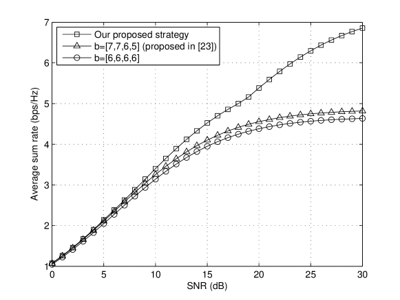
Figure 4: Sum rates of a $4\times 4$ MIMO BC using various feedback rate sharing strategies ($\sum b_{k}=24$). Different path losses among the users are considered $(\gamma_{1},\gamma_{2},\gamma_{3},\gamma_{4})=(1.5,1.25,1,0.75)$.

Consider a $4\times 4$ MIMO BC with 24 total allowable feedback bits ($K\bar{b}=24$). We assume the path losses of each user as $(\gamma_{1},\gamma_{2},\gamma_{3},\gamma_{4})=(1.5,1.25,1,0.75)$. For the given path losses, the feedback rate sharing strategy given in (22) becomes $\mathbf{b}=[7,7,6,4]$. On the other hand, the optimal feedback rate strategy obtained by the proposed numerical method is given in Table II according to various SNR regions. The average sum rate by the optimal feedback rate strategy by the proposed method is plotted in Fig 4. Fig 4 confirms that our proposed strategy given in Table II more significantly outperforms the feedback rate sharing strategy proposed in (22) as SNR becomes higher.

IV-E Complexity Analysis

In this subsection, we analyze complexity to find the optimal feedback rate strategy described in Algorithm 1. Because the effects of different path losses can be simply regarded as different transmit SNR of users as described in Section IV-D, the achievable rates of users with different path losses can be calculated by the same procedure based on Fig. 3.

In the symmetric path loss cases (i.e., $\gamma_{1}=\ldots=\gamma_{K}$), two strategies $\mathbf{b}_{1}$ and $\mathbf{b}_{2}$ yield the same performance whenever $\mathbf{b}_{1}^{\downarrow}=\mathbf{b}_{2}^{\downarrow}$. Thus, the optimal feedback strategy can be found in the strategy set $\mathcal{B}$ given by

$$\mathcal{B}=\Big{\{}\mathbf{b}^{\downarrow}~{}\Big{|}~{}\mathbf{b}\in(\mathbb{Z}^{+}\cup\{0\})^{K},~{}\sum_{k=1}^{K}[\mathbf{b}]_{k}=K\bar{b}\Big{\}}.$$ (23)

The number of all possible strategies is determined by the total feedback size as in Table III.

TABLE III: The number of feedback strategies for $4\times 4$ MIMO BC

Total FB Size	8	16	24	32	40	48	56	64
$|\mathcal{B}|$	15	64	169	351	632	1033	1575	2280

For asymmetric path loss cases, without loss of generality we consider the case that $\gamma_{1}\geq\ldots\geq\gamma_{K}$. Because the larger feedback size yields the higher multiplexing gain, larger feedback size should be assigned to the user with smaller path loss (i.e., larger $\gamma_{k}$). This implicates that the strategy $\mathbf{b}^{\downarrow}$ outperforms $\mathbf{b}$, i.e.,

$$\sum_{k=1}^{K}\mathcal{R}_{k}(\gamma_{k}P,[\mathbf{b}^{\downarrow}]_{k})\geq\sum_{k=1}^{K}\mathcal{R}_{k}(\gamma_{k}P,[\mathbf{b}]_{k}).$$

Therefore, the optimal feedback rate sharing strategy is selected in the feedback strategy set $\mathcal{B}$ defined in (23). Because the number of all possible strategies, i.e., $|\mathcal{B}|$, is the same for the symmetric and the asymmetric path loss cases, the computational complexity is also the same for both cases.

IV-F Extension to Stream Control

Although the equal power allocation with full multiplexing is mainly considered in our manuscript, our feedback rate sharing strategy can readily be extended to the stream control where the transmitter adaptively controls multiplexing gain. For $4\times 4$ MIMO BC, for example, four ways of equal power allocation according to the number of streams – $[P/4,P/4,P/4,P/4]$, $[P/3,P/3,P/3,0]$, $[P/2,P/2,0,0]$, and $[P,0,0,0]$ – are possible with the steam control. Note that single stream transmission corresponds to the TDMA scheme. Since we consider ZF beamforming at the transmitter, the beamforming vector for each user is randomly picked orthogonal to other users’ quantized channels. Therefore, it can easily be shown that Theorem 1 and Theorem 2 are still valid even with the stream control. In Table I, we have found the optimal feedback rate sharing strategy for $4\times 4$ MIMO BC according to the number of streams and SNR when total feedback budget is 24bits and the path losses are symmetric. We can also find the optimal feedback rate sharing strategies for asymmetric path losses because Lemma 2 still holds for the stream control and hence the rate of each served user is affected by its own feedback size.

V Numerical Results

V-A Numerical Examples

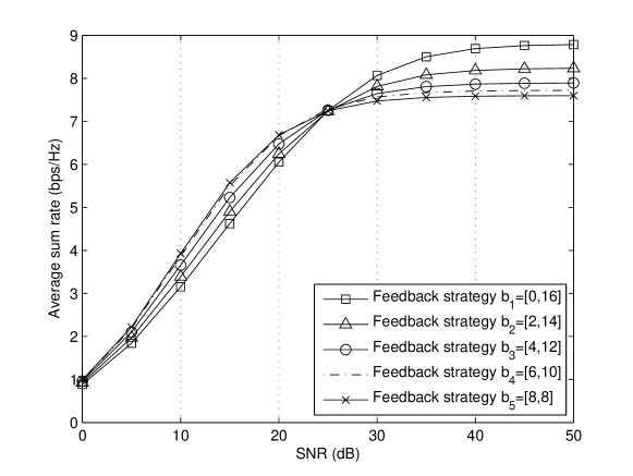
Figure 5: Sum rates of a $2\times 2$ MIMO BC using various feedback rate sharing strategies ($\sum b_{k}=16$).

In this section, we present numerical results to analyze the effects of feedback rate sharing strategies. In Fig. 5, the average sum rates of a $2\times 2$ MIMO BC using different feedback rate sharing strategies. We consider five feedback rate sharing strategies $(\mathbf{b}_{1},\mathbf{b}_{2},\mathbf{b}_{3},\mathbf{b}_{4},\mathbf{b}_{5})=([0,16],[2,14],[4,12],[6,10],[8,8]$) such that $\mathbf{b}_{1}\succeq\mathbf{b}_{2}\succeq\mathbf{b}_{3}\succeq\mathbf{b}_{4}\succeq\mathbf{b}_{5}$. In Fig. 5, for all $\mathbf{b}_{i}\succeq\mathbf{b}_{j}$ we obtain $\lim_{P\to 0}\mathcal{R}(P,\mathbf{b}_{i})<\lim_{P\to 0}\mathcal{R}(P,\mathbf{b}_{j})$ and $\lim_{P\to\infty}\mathcal{R}(P,\mathbf{b}_{i})>\lim_{P\to\infty}\mathcal{R}(P,\mathbf{b}_{j})$ as stated in Theorem 1 and Theorem 2, respectively. In the low SNR region, the equal sharing of the sum feedback rate $\mathbf{b}_{5}=[8,8]$ achieves the highest average sum rate while allocating the whole feedback rate to a single user $\mathbf{b}_{1}=[0,16]$ achieves the lowest average sum rate as predicted in Corollary 1. In the high SNR region, however, allocating the whole feedback rate to a single user $\mathbf{b}_{1}=[0,16]$ achieves the highest achievable rate whereas equal sharing of the feedback rate $\mathbf{b}_{5}=[8,8]$ achieves the worst achievable rate as claimed in Corollary 2.

In a noise limited environment, increasing multiplexing gains directly results in higher sum rate, and the multiplexing gains are maximized when the feedback rate is equally shared among users. Since the remaining interference caused by the quantization error becomes dominant in the high SNR region, the full multiplexing gain cannot be achieved and the multiplexing gain rather diminishes as SNR increases. Therefore, by allocating the whole feedback rate to a single user, the other users can effectively eliminate the interference limitation by removing all multiuser interference from the user being allocated the whole feedback rate. Reducing the number of interferers is more effective in an interference limited environment from a sum rate perspective since the multiplexing gain is already lost.

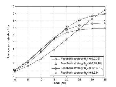
(a) Random vector codebook.

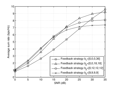
(b) Spherical cap codebook.

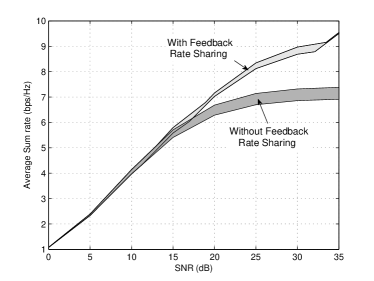
(c) The conjectured average sum rate region for practical quantization codebook.

Figure 6: Sum rates of a $4\times 4$ MIMO BC using various feedback rate sharing strategies ($\sum b_{k}=36$).

The sum rate of a $4\times 4$ MIMO BC for various feedback sizes is shown in Fig.6(a) where the total feedback rate is restricted to 36 bits. Four feedback rate sharing strategies are considered – $(\mathbf{b}_{1},\mathbf{b}_{2},\mathbf{b}_{3},\mathbf{b}_{4})$ = ($[0,0,0,36]$, $[0,0,18,18]$, $[0,12,12,12]$, $[9,9,9,9]$) such that $\mathbf{b}_{1}\succeq\mathbf{b}_{2}\succeq\mathbf{b}_{3}\succeq\mathbf{b}_{4}$. As stated in Theorem 1 and Theorem 2, we can observe that $\lim_{P\to 0}\mathcal{R}(P,\mathbf{b}_{i})<\lim_{P\to 0}\mathcal{R}(P,\mathbf{b}_{j})$ and $\lim_{P\to\infty}\mathcal{R}(P,\mathbf{b}_{i})>\lim_{P\to\infty}\mathcal{R}(P,\mathbf{b}_{j})$ whenever $\mathbf{b}_{i}\succeq\mathbf{b}_{j}$. Also, we can observe that the equal allocation to the optimal number of users according to SNR becomes the optimal strategy in the mid-SNR region as stated in Observation 1.

V-B Extension to Other Codebook Models

Although the overall trends obtained by RVQ are known to agree well with the results of other codebooks, we consider another codebook model to verify the observations and conclusions obtained for RVQ are effective for other codebook models. Since a rate maximizing codebook is difficult to find, we consider a spherical cap codebook [27, 3, 14] which is based on an ideal assumption that each quantization cell in $b$-bit codebook is a spherical cap with the surface area $2^{-b}$. A spherical cap codebook is an ideal vector quantizer whose quantization error is stochastically dominated by any other codebooks [8]. In a $b$-bit spherical cap codebook, the CDF of the quantization error denoted by $\tilde{Z}$ becomes

$$\mathrm{Pr}[\tilde{Z}<z]=\bigg{\{}\begin{array}[]{ll}2^{b}z^{M-1},&\quad 0\leq z\leq 2^{-\frac{b}{M-1}}\\ 1,&\quad z\geq 2^{-\frac{b}{M-1}}.\end{array}$$ (25)

Fig. 6(a) and Fig. 6(b) show the average sum rates of a $4\times 4$ MIMO BC using various feedback sharing strategies when RVQ and a spherical cap codebook are used, respectively. This result confirms the optimal strategies obtained from RVQ is still valid for the spherical cap codebook.

In general, RVQ and spherical cap codebook are regarded as the lower bound and the upper bound of the practical quantization codebook, respectively. From the both codebook models, therefore, we can conjecture the average sum rate in practical $4\times 4$ ZF MIMO BC for the given configuration. In Fig. 6(c), the conjectured average sum rate region for practical quantization codebook (with $\sum b_{k}=36$) is shaded with/without adopting our proposed feedback rate sharing strategy, respectively. Each shaded region is bounded both on RVQ and the spherical cap cases plotted in Fig. 6(a) and Fig. 6(b), respectively. Fig. 6(c) implicates that our proposed feedback rate sharing strategy is useful even for practical ZF MIMO BC systems, especially in the high SNR region.

V-C Comparison with TDMA and Regularized ZF

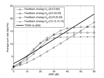
(a) ZF beamforming vs. TDMA

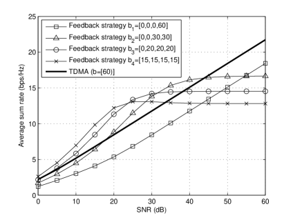
(b) Regularized ZF beamforming vs. TDMA

Figure 7: Sum rates of a $4\times 4$ MIMO BC using various feedback rate sharing strategies ($\sum b_{k}=60$).

We also consider the regularized zero-forcing beamforming [8] which enhances the performance of ZF beamforming in the low SNR region. Also, TDMA is considered and compared with both ZF beamforming and regularized ZF beamforming. The average sum rates of a $4\times 4$ MIMO BC using ZF beamforming adopting our proposed feedback rate sharing strategy are compared with TDMA in Fig. 7(a), when $\sum b_{k}=60$. In TDMA, all available feedback bits are allocated to the single served user ($\mathbf{b}=[60]$). In Fig. 7(a), we can observe that ZF beamforming is inferior to a TDMA system in both low and high SNR regions although it outperforms a TDMA system in the mid SNR region. In these regions, it is desirable to adopt the mode switching [31] between ZF and TDMA for sum rate maximization.

In the regularized ZF beamforming, the normalized column vectors of $\hat{\mathbf{H}}^{\dagger}\left(\hat{\mathbf{H}}\hat{\mathbf{H}}^{\dagger}+\frac{M}{P}\mathbf{I}_{M}\right)^{-1}$ are used for the beamforming vectors where $\mathbf{I}_{M}$ is an $M\times M$ identity matrix. Although the optimal feedback rate sharing strategy using the regularized ZF beamforming is hard to analyze, the feedback rate sharing strategy will be the same with that of ZF beamforming case in the high SNR region. This is because the regularized ZF beamforming vectors correspond to ZF beamforming vectors in the high SNR region. In Fig. 7(b), the average sum rates of a $4\times 4$ MIMO BC using regularized ZF beamforming are plotted while other parameters are same in Fig. 7(a). As shown in Fig. 7(b), the regularized ZF beamforming improves ZF beamforming especially in the low SNR region and hence outperforms TDMA in wider SNR region.

Since TDMA always achieves a multiplexing gain of one even with blind transmission, TDMA system outperforms MIMO BC with limited feedback in the high SNR region. This is because the achievable rate of MIMO BC with finite limited feedback is saturated in the high SNR region due to mutual interference. The inferior performance in the high SNR region is a fundamental limit of MIMO BC with limited feedback. However, it should be noted that ZF beamforming can be enhanced by the regularized ZF beamforming and our feedback rate sharing strategy enables ZF beamforming or regularized ZF beamforming to outperform TDMA in wider SNR region. Note that our main contributions are to find the feedback rate sharing strategy and to show the feedback rate sharing strategy (e.g., $\sum b_{k}=60$) enhances the system performance compare to equal feedback rate sharing (e.g. $\mathbf{b}=[15,15,15,15]$). In Fig. 7(b), the regularized ZF beamforming outperforms TDMA from -15dB to about 45dB when the optimal feedback rate sharing strategy is employed, whereas equally sharing makes the regularized ZF beamforming outperform TDMA until about 34dB.

VI Conclusion

In this paper, we have analyzed the average sum rate of ZF MIMO BC with limited feedback when the users share the feedback rates. The impact of asymmetric feedback sizes among the users has been rigorously analyzed by adopting RVQ at each user. Our mathematical analysis has shown that the optimal feedback rate sharing strategy in the high SNR region is to allocate the whole feedback rate to a single user. On the other hand, the optimal feedback rate sharing strategy in the low SNR region is the equal sharing of the feedback rate among users. We have proposed a simple numerical method for finding the optimal feedback rate sharing strategy in the practical SNR region and shown that equal sharing of the feedback rate among the optimal number of concurrent users is optimal. It has also been shown that the proposed numerical method can be applicable to finding the optimal feedback rate sharing strategy when path losses of the users are different. In the simulation part, we have shown our proposed feedback capacity sharing strategy is still valid for other system configurations such as regularized zeroforcing transmission and spherical-cap codebook.

Appendix A. Proof of Lemma 1

Since the channel vectors are i.i.d, it is obvious that $Q_{k}\sim Q_{1}$ for all $k$. Because $\mathbf{h}_{k}$ is isotropic in $\mathbb{C}^{M}$, the quantization of $\mathbf{h}_{k}$ is also isotropic in $\mathbb{C}^{M}$. Thus, $\{\hat{\mathbf{h}}_{k}\}_{k=1}^{K}$ become independent and isotropically distributed random vectors in $\mathbb{C}^{M}$. Because $\mathbf{v}_{k}$ is uniquely obtained from $\{\hat{\mathbf{h}}_{i}\}_{i\neq k}$, the beamforming vectors, $\{\mathbf{v}_{k}\}_{k\neq 1}^{K}$, are also isotropic in $\mathbb{C}^{M}$. Since $\mathbf{v}_{k}$ is independent of $\hat{\mathbf{h}}_{k}$, $X_{k}(=|\tilde{\mathbf{h}}_{k}\mathbf{v}_{k}|^{2})$ becomes the squared inner product between two independent random vectors isotropic in $\mathbb{C}^{M}$. Hence, $X_{k}$ is identical for all $k$, i.e., $X_{k}\sim X_{1}$. For $W_{k}(=\sum_{i\neq k}|\mathbf{e}_{k}^{\dagger}\mathbf{v}_{i}|^{2})$, both $\mathbf{e}_{k}$ and $\{\mathbf{v}_{i}\}_{i\neq k}$ are picked independently in the null space of $\hat{\mathbf{h}}_{k}$, and they are also isotropic in the $M-1$ dimensional subspace. Thus, $W_{k}$ becomes the sum of $K-1$ the squared inner products between two independent and isotropic random vectors in the $M-1$ dimensional subspace in $\mathbb{C}^{M}$ so that $W_{k}\sim W_{1}$, $\forall k$. From above reasons, we can conclude that $Q_{k}$, $X_{k}$, and $W_{k}$ are identical for all $k$, respectively, invariant with the feedback sizes $b_{1},\ldots,b_{K}$.

We can prove the second property that $\{Q_{k},X_{k},W_{k}\}_{k=1}^{K}$ is independent of all $\{Z_{k}\}_{k=1}^{K}$ because $Z_{k}$ is only dependent on $b_{k}$ as shown in (2).

Because $\{Q_{i},X_{i},W_{i}\}$ is interchangebly obtained from $\{Q_{k},X_{k},W_{k}\}$ by swapping the index of $\mathbf{h}_{i}$ and $\mathbf{h}_{k}$ whose distribution are the same, i.e., $Q_{i}\sim Q_{k}$, $X_{i}\sim X_{k}$, and $W_{i}\sim W_{k}$, we can obtain the third property such that

$$f_{Q_{k},X_{k},W_{k}}(q,x,w)=f_{Q_{1},X_{1},W_{1}}(q,x,w),\quad k=1,\ldots,K.$$

When all users use the equal feedback size, (i.e., $Z_{k}\sim\bar{Z}$, $\forall k$), the average achievable rate of each user is the same such that $\mathbb{E}\left[\log_{2}\left(1+\frac{\frac{P}{M}Q_{k}X_{k}}{1+\frac{P}{M}Q_{k}W_{k}\bar{Z}}\right)\right]=\mathbb{E}\left[\log_{2}\left(1+\frac{\frac{P}{M}Q_{1}X_{1}}{1+\frac{P}{M}Q_{1}W_{1}\bar{Z}}\right)\right]$ for all $k$. This can be explained from the fact that $f_{Q_{k},X_{k},W_{k},\bar{Z}}(q,x,w,z)\stackrel{{\scriptstyle(a)}}{{=}}f_{Q_{k},X_{k},W_{k}}(q,x,w)f_{\bar{Z}}(z)\stackrel{{\scriptstyle(b)}}{{=}}f_{Q_{1},X_{1},W_{1}}(q,x,w)f_{\bar{Z}}(z)\stackrel{{\scriptstyle(a)}}{{=}}f_{Q_{1},X_{1},W_{1},\bar{Z}}(q,x,w,z)$ where $(a)$ and $(b)$ are from the second property and the third property, respectively.

Appendix B. Proof of Theorem 1

To prove Theorem 1, we firstly show the average quantization error $\mathbb{E}[Z_{k}]$ is a discretely convex function of $b_{k}$. Then, we use the majorization theory. We start from following Lemma.

Lemma 3.

The average quantization error $\mathbb{E}[Z_{k}]$ is a discretely convex function of $b_{k}$.

Proof.

It was shown in [8, 28] that $\mathbb{E}[Z_{k}|b_{k}=b]=2^{b}\cdot\beta\left(2^{b},\frac{M}{M-1}\right)$, where $\beta(x,y)$ is the beta function given by $\beta(x,y)=\frac{\Gamma(x)\Gamma(y)}{\Gamma(x+y)}$. Using this, we obtain

$$\mathbb{E}[Z_{k}|b_{k}=b+1]$$

$$=2^{b+1}\cdot\beta\left(2^{b+1},\frac{M}{M-1}\right)$$

$$=\frac{2\cdot\Gamma\left(2^{b+1}\right)\Gamma\left(2^{b}+\frac{M}{M-1}\right)}{\Gamma\left(2^{b}\right)\Gamma\left(2^{b+1}+\frac{M}{M-1}\right)}\times\frac{2^{b}\cdot\Gamma\left(2^{b}\right)\Gamma\left(\frac{M}{M-1}\right)}{\Gamma\left(2^{b}+\frac{M}{M-1}\right)}$$

$$\stackrel{{\scriptstyle(a)}}{{=}}\frac{2\cdot\prod_{i=2^{b}}^{2^{b+1}-1}i}{\prod_{i=2^{b}}^{2^{b+1}-1}\big{(}i+\frac{M}{M-1}\big{)}}\times\mathbb{E}[Z_{k}|b_{k}=b],$$

where the equality $(a)$ is from $\Gamma(x+1)=x\Gamma(x)$. Thus, we can rewrite $\mathbb{E}[Z_{k}|b_{k}=b+1]=\eta_{b}\cdot\mathbb{E}[Z_{k}|b_{k}=b]$ where $\eta_{b}\triangleq 2\cdot\prod_{i=2^{b}}^{2^{b+1}-1}\frac{i}{\big{(}i+\frac{M}{M-1}\big{)}}$.

When we define a forward difference function $\Delta(b)\triangleq\mathbb{E}[Z_{k}|b_{k}=b+1]-\mathbb{E}[Z_{k}|b_{k}=b]$, we can find that the forward difference function is an increasing function of $b$, i.e., $\Delta(b+1)>\Delta(b)$, such that

$$\Delta(b+1)-\Delta(b)$$

$$=\mathbb{E}[Z_{k}|b_{k}=b+2]-2\cdot\mathbb{E}[Z_{k}|b_{k}=b+1]+\mathbb{E}[Z_{k}|b_{k}=b]$$

$$=(\eta_{b+1}\eta_{b}-2\eta_{b}+1)\cdot\mathbb{E}[Z_{k}|b_{k}=b]\stackrel{{\scriptstyle(a)}}{{>}}0$$

where $(a)$ is from the fact that $\eta_{b+1}\eta_{b}-2\eta_{b}=4\cdot\left(\prod_{i=2^{b}}^{2^{b+2}-1}\frac{i}{\big{(}i+\frac{M}{M-1}\big{)}}-\prod_{i=2^{b}}^{2^{b+1}-1}\frac{i}{\big{(}i+\frac{M}{M-1}\big{)}}\right)$ is ranged in $[-1,0]$ and minimized and maximized when $M=2$ and $M=\infty$, respectively. Since a discretely convex function has an increasing (non-decreasing) forward difference function [30], $\mathbb{E}[Z_{k}]$ is a discretely convex function of $b_{k}$. ∎

It is widely known in majorization theory that for a convex function $h:\mathbb{R}\to\mathbb{R}$ and two vectors $\mathbf{a}_{1},\mathbf{a}_{2}\in\mathbb{R}^{n}$,

$$\sum_{i=1}^{n}h([\mathbf{a}_{1}]_{i})\leq\sum_{i=1}^{n}h([\mathbf{a}_{2}]_{i}),$$ (B.1)

whenever $\mathbf{a}_{1}\preceq\mathbf{a}_{2}$. In the low SNR region, the sum average rate with feedback rate sharing strategy is only related with $\sum_{k=1}^{K}\mathbb{E}[Z_{k}]$ as stated in (14). From Lemma 3, we know the average quantization error is a convex function of $b_{k}$. With the feedback rate sharing strategies $\mathbf{b}_{1}\preceq\mathbf{b}_{2}$, therefore, we can conclude that

$$\sum_{k=1}^{K}\mathbb{E}\{Z_{k}|b_{k}=[\mathbf{b}_{1}]_{k}\}\leq\sum_{k=1}^{K}\mathbb{E}\{Z_{k}|b_{k}=[\mathbf{b}_{2}]_{k}\},$$ (B.2)

and equivalently, $\lim_{P\to 0}\mathcal{R}(P,\mathbf{b}_{1})>\lim_{P\to 0}\mathcal{R}(P,\mathbf{b}_{2})$.

Appendix C. Proof of Theorem 2

We firstly show that $\mathbb{E}\left[\log_{2}Z_{k}\right]$ is a discretely concave function of $b_{k}$ in following lemma.

Lemma 4.

The average quantization error $\mathbb{E}[\log_{2}Z_{k}]$ is a discretely concave function of $b_{k}$.

Proof.

In [8], it was shown that $\mathbb{E}\left[\log_{2}Z_{k}|b_{k}=b\right]=\frac{-\log_{2}e}{M-1}\sum_{i=1}^{2^{b}}\frac{1}{i}$. In this case, the forward difference function $\Delta(b)\triangleq\mathbb{E}\left[\log_{2}Z_{k}|b_{k}=b+1\right]-\mathbb{E}\left[\log_{2}Z_{k}|b_{k}=b\right]$ becomes

$$\Delta(b) =\frac{-\log_{2}e}{M-1}\sum_{i=2^{b}+1}^{2^{(b+1)}}\frac{1}{i},$$ (C.1)

and is a monotonically decreasing function of $b$, i.e., $\Delta(b)>\Delta(b+1)$. Since a discretely concave function has a decreasing(non-increasing) forward difference function [30], $\mathbb{E}[\log_{2}Z_{k}]$ is a discretely concave function of $b_{k}$. ∎

In majorization theory, for a concave function $g:\mathbb{R}\to\mathbb{R}$, it satisfies that

$$\sum_{i=1}^{n}g([\mathbf{a}_{1}]_{i})\geq\sum_{i=1}^{n}g([\mathbf{a}_{2}]_{i})$$ (C.2)

whenever two vectors $\mathbf{a}_{1},\mathbf{a}_{2}\in\mathbb{R}^{n}$ satisfies $\mathbf{a}_{1}\preceq\mathbf{a}_{2}$. In the high SNR region, the average sum rate with feedback rate sharing strategy is related with $\sum_{k=1}^{K}\mathbb{E}[\log_{2}Z_{k}]$ as stated in (18). As stated in Lemma 4, $\mathbb{E}[\log_{2}Z_{k}]$ is the concave function of $b_{k}$. Thus, under the feedback rate sharing strategies $\mathbf{b}_{1}\preceq\mathbf{b}_{2}$, we can conclude that

$$\sum_{k=1}^{K}\mathbb{E}\{\log_{2}Z_{k}|b_{k}=[\mathbf{b}_{1}]_{k}\}\geq\sum_{k=1}^{K}\mathbb{E}\{\log_{2}Z_{k}|b_{k}=[\mathbf{b}_{2}]_{k}\},$$

equivalently, $\lim_{P\to\infty}\mathcal{R}^{-}(P,\mathbf{b}_{1})>\lim_{P\to\infty}\mathcal{R}^{-}(P,\mathbf{b}_{2})$. As stated in Section IV-B, in the high SNR region, the achievable rate at each user is dominated by the rate decreasing term. Thus, we conclude that the feedback rate sharing strategy $\lim_{P\to\infty}\mathcal{R}(P,\mathbf{b}_{1})<\lim_{P\to\infty}\mathcal{R}(P,\mathbf{b}_{2})$ for feedback rate sharing strategies $\mathbf{b}_{1}\preceq\mathbf{b}_{2}$.

References

- [1] G. Caire and S. Shamai (Shitz), “On the achievable throughput of a multiantenna gaussian broadcast channel,” IEEE Trans. Inf. Theory, vol. 49, no. 7, pp. 1691–1706, July 2003.
- [2] P. Viswanath and D. N. C. Tse, “Sum capacity of the vector gaussian broadcast channel and downlink-uplink duality,” IEEE Trans. Inf. Theory, vol. 49, no. 8, pp. 1912–1921, Aug. 2003.
- [3] H. Weingarten, Y. Steinberg, and S. Shamai (Shitz), “The capacity region of the gaussian multiple-input multiple-output broadcast channel,” IEEE Trans. Inf. Theory, vol. 52, no. 9, pp. 3936–3964, Sep. 2006.
- [4] M. Costa, “Writing on dirty paper,” IEEE Trans. Inf. Theory, vol. IT-29, pp. 439–441, May 1983.
- [5] T. Yoo and A. Goldsmith, “On the optimzlity of multiantenna broadcast scheduling using zero-forcing beamforming,” IEEE J. Sel. Areas Commun., vol. 24, no. 3, pp. 528–541, Mar. 2006.
- [6] R. Zamir, S. S. (Shitz), and U. Eres, “Nested linear/lattice codes for structured multiterminal binning,” IEEE Trans. Inf. Theory, vol. 48, no. 6, pp. 1250–1277, June 2002.
- [7] D. J. Love, R. W. Heath., W. Santipach, and M. L. Honig, “What is the value of limited feedback for MIMO channels?” IEEE Commun. Mag., vol. 42, no. 10, pp. 54–59, Oct. 2004.
- [8] N. Jindal, “MIMO broadcast channels with finite-rate feedback,” IEEE Trans. Inf. Theory, vol. 52, no. 11, pp. 5045–5060, Sep. 2006.
- [9] N. Ravindran and N. Jindal, “Limited feedback-based block diagonalization for the MIMO broadcast channel,” IEEE J. Sel. Areas Commun., vol. 26, no. 8, pp. 1473–1482, Oct. 2008.
- [10] Y. Cheng, V. K. N. Lau, and Y. Long, “A scalable limited feedback design for network MIMO using per-cell product codebook,” IEEE Trans. Wireless Commun., vol. 9, no. 10, pp. 3093–3099, Oct. 2010.
- [11] I. H. Kim, S. Y. Park, D. J. Love, and S. J. Kim, “Improved multiuser MIMO unitary precoding using partial channel state information and insights from the Riemannian manifold,” IEEE Trans. Wireless Commun., vol. 8, no. 8, pp. 4014–4023, Aug. 2009.
- [12] N. Jindal, “Antenna combining for the MIMO downlink channel,” IEEE Trans. Wireless Commun., vol. 7, no. 10, pp. 3834–3844, Oct. 2008.
- [13] M. Sharif and B. Hassibi, “On the capacity of MIMO broadcast channels with partial side information,” IEEE Trans. Inf. Theory, vol. 51, no. 2, pp. 506–522, Feb. 2005.
- [14] T. Yoo, N. Jindal, and A. Goldsmith, “Multi-antenna downlink channels with limited feedback and user selection,” IEEE J. Sel. Areas Commun., vol. 25, no. 7, pp. 1478–1491, Sep. 2007.
- [15] W. Choi, A. Forenza, J. G. Andrews, and R. W. Heath, “Opportunistic space division multiple access with beam selection,” IEEE Trans. Wireless Commun., vol. 6, no. 12, pp. 2371–2380, Dec. 2007.
- [16] C. K. Au-Yeung, S. Y. Park, and D. J. Love, “A simple dual-mode limited feedback multiuser downlink system,” IEEE Trans. Commun., vol. 57, no. 5, pp. 1514–1522, May 2009.
- [17] Y. Huang and B. D. Rao, “An analytical framework for heterogeneous partial feedback design in heterogeneous multicell OFDMA networks,” IEEE Trans Sig. Proc., vol. 61, no. 3, pp. 753–769, Feb. 2013.
- [18] K. Huang, R. W. Heath, and J. G. Andrews, “Space division multiple access with a sum feedback rate constraint,” IEEE Trans. Sig. Proc., vol. 55, no. 7, pp. 3879–3891, July 2007.
- [19] N. Ravindran and N. Jindal, “Multi-user diversity vs. accurate channel state information in MIMO downlink channels,” IEEE Trans. Wireless Commun., vol. 11, no. 9, pp. 3037–3046, Sep. 2012.
- [20] R. Bhagavatula and R. W. Heath, “Adaptive limited feedback for sum-rate maximizing beamforming in cooperative multicell systems,” IEEE Trans. Sig. Procs., vol. 59, no. 2, pp. 800–811, Feb. 2011.
- [21] K. Huang, V. K. N. Lau, and D. Kim, “Stochastic control of event-driven feedback in multi-antenna interference channels”, IEEE Trans. Sig. Proc., vol. 59, no. 12, pp. 6112–6126, Dec. 2011.
- [22] B. Clerckx, G. Kim, J. Choi, S. Kim, “Allocation of feedback bits among users in broadcast MIMO channels”, in Proc of IEEE Global Telecommunications Conference (GLOBECOM), Dec. 2008.
- [23] W. Xu, C. Zhao, and Z. Ding, “Optimisation of limited feedback design for heterogeneous users in multi-antenna downlinks,” IET Commun., vol. 3, no. 11, pp. 1724–1735, Nov. 2009.
- [24] B. Khoshnevis and W. Yu, “Bit allocation laws for multi-antenna channel quantization: Multi-user case,” IEEE Trans. Signal Process. vol. 60, no. 1, Jan. 2012.
- [25] J. H. Lee and W. Choi, “Feedback rate sharing in MIMO broadcast channels,” in Proc. of IEEE International Conference on ITS Telecommunication (ITST), Lille, France, Oct. 2009.
- [26] W. Santipach and M. L. Honig, “Signature optimization for CDMA with limited feedback,” IEEE Trans. Inf. Theory, vol. 51, no. 10, pp. 3475–3492, Oct. 2005.
- [27] K. Mukkavilli, A. Sabharwal, E. Erkip, and B. Aazhang, “On beamforming with finite rate feedback in multiple-antenna systems,” IEEE Trans. Inf. Theory, vol. 49, no. 10, pp. 2562–2579, Oct. 2003.
- [28] C. K. Au-Yeung and D. J. Love, “On the performance of random vector quantization limited feedback beamforming in a MISO system,” IEEE Trans. Wireless Commun., vol. 6, no. 2, pp. 458–462, Feb. 2007.
- [29] D. Zwillinger, CRC standard mathematical tables and formulae, 31st ed. Boca Raton, FL: Chapman & Hall/CRC, 2003.
- [30] Ü. Yüceer, “Discrete convexity: convexity for functions defined on discrete spaces,” Discrete Applied Mathematics, vol. 119/3, pp. 297–304, 2002.
- [31] J. Zhang , R. W. Heath Jr., M. Kountouris and J. G. Andrews, “Mode switching for the multi-antenna broadcast channel based on delay and channel quantization,” EURASIP J. Adv. Signal Process. (Special Issue Multiuser Lim. Feedback), 2009, article ID 802548, 15 pages.