The three site interacting spin chain in staggered field: Fidelity vs Loschmidt echo

Abstract

We study the the ground state fidelity and the ground state Loschmidt echo of a three site interacting XX chain in presence of a staggered field which exhibits special types of quantum phase transitions due to change in the topology of the Fermi surface, apart from quantum phase transitions from gapped to gapless phases. We find that on one hand, the fidelity is able to detect only the boundaries separating the gapped from the gapless phase; it is completely insensitive to the phase transition from two Fermi points region to four Fermi points region lying within this gapless phase. On the other hand, Loschmidt echo shows a dip only at a special point in the entire phase diagram and hence fails to detect any quantum phase transition associated with the present model. We provide appropriate arguments in support of this anomalous behavior.

I Introduction

The desire of building a quantum computer to solve quantum problems efficiently has lead to an immense recent development in the studies of quantum information theory in many body systems and its connection to quantum phase transitions. Many important quantum information theoretic measures exhibit interesting scaling behavior close to a quantum critical point (QCP) of a quantum many body system. One such measure is the ground state quantum fidelity, which is an overlap of the ground state wave function at two different values of the parameters of the quantum Hamiltonian zanardi06 ; zhou08 ; gu10 ; dutta10 ; sacramento11 ; damski12 . The fidelity has attracted the attention of the condensed matter physicists in recent years because of its ability to detect a quantum critical point without an a priori knowledge of the order parameter of the system, which otherwise is the conventional way of probing a quantum phase transition (QPT)sachdev99 ; chakrabarti96 ; dutta10 . The quantum fidelity shows a dip at a QCP while the fidelity susceptibility (which defines the rate at which the fidelity changes for a finite system in the limit when the two parameters under consideration are infinitesimally close in the parameter space) shows a peak right there and has a scaling form given in terms of some of the exponents associated with the corresponding QPT gu10 . Similarly, the fidelity has been conjectured to exhibit an interesting scaling relation involving the quantum critical exponents also in the thermodynamically large system for a finite separation between the parameters rams11 .

Although approaches based on the fidelity and the fidelity susceptibility have been successful in detecting various types of quantum phase transition points, for example, ordinary critical points separating two gapped phases through a gapless pointzanardi06 ; zhou08 or topological QPTsyang08 or QPT in Bose Hubbard model buonsante07 , but its usefulness in a general scenario is not yet fully settled. The absence of a peak in the fidelity susceptibility when $\nu d>2$ (where $\nu$ is the correlation length exponent associated with the QCP of $d$-dimensional system) has been argued in Refs. nofidelity, ; manisha12, . It has also been shown that in the marginal case ($\nu d=2$), a sharp dip in the fidelity is absent at the QCP using the example of Dirac points in two dimensionspatel13 . On the other hand, the presence of a quasi-periodic lattice introduces extra peaks in fidelity susceptibility which can not be detected by studying the energy spectrum manisha12 . To show one more contradiction, we present a model where the fidelity detects the onset of a gapless quantum critical region but not the transition between two different phases within this gapless quantum critical region.

One of the other important quantities which bridges a connection between the quantum information theory and QPT is the ground state Loschmidt echo ($L$) quan06 ; cucchietti07 ; mukherjee12 . The Loschmidt echo is the measure of the overlap (at an instant $t$) of the same initial state, the ground state of the initial Hamiltonian of a many body system $H(\lambda)$, but evolving under the influence of the two Hamiltonians, $H(\lambda)$ and $H(\lambda+\delta)$; in this sense, it is the dynamical counterpart of the static fidelity zanardi06 . This $L$ also shows a dip at the QCP, thus enabling us to detect it. From the viewpoint of quantum information theory, Loschmidt echo can be used to measure the quantum to classical transition (or the transition from a pure to the mixed state) of a qubit coupled to an environment consisting of the many-body system. In this case, it is the interaction between the qubit and the many body system that changes the parameter $\lambda$ of the Hamiltonian to $\lambda+\delta$ quan06 . The notion of the $L$ was actually introduced in connection to the quantum to classical transition in quantum chaos peres95 ; jalabert01 ; karkuszewski02 ; cerruti02 ; cucchietti03 and now extended to various other systems undergoing a QPT like Ising model quan06 , Bose-Einstein condensate model zheng08 and Dicke modelhuang09 . It has also been studied experimentally using NMR experiments buchkremer00 ; zhang09 ; sanchez09 .

In this paper, we point out the inability of the fidelity or the $L$ to detect certain special class of QCPs by taking the example of staggered transverse field in a three spin interacting spin-1/2 XX chain titvinidze03 . There are several studies which explore the phase transition in similar or slightly different three site interacting Hamiltonians using tools like zero and finite temperature magnetization and magnetization susceptibility titvinidze03 ; threespin1 and transport properties like spin Drude weight and thermal Drude weight threespin1 ; lou04 . The effect of three site interaction has also been studied using magnetocaloric effect topilko12 or by using dynamic structure factors of the ground state krokhmalskii08 . On the other hand, the effect of three site interacting Hamiltonian is relatively less explored using quantum information theoretic measures which is the focus of the present paper. There have been studies using Renyi entropy eloy12 , concurrence, geometric discord and quantum discord cheng12 , average fidelity of state transfer hu12 , geometric phase zhang12 , $L$ lian11 and fidelity liu12 of different versions of three site interacting Hamiltonian. This study is an important addition to the literature as to the best of our knowledge, the fidelity and the $L$ of a Hamiltonian which also undergoes a very unique type of quantum phase transition, namely, from two Fermi points to four Fermi points, has not been investigated before.We find surprising results due to the combined effect of staggered field and three site interacting term in the calculations of fidelity and $L$ which are not a priori obvious. It is worth mentioning here that many interesting experimental observations, like magnetic properties of solid ${}^{3}\rm{He}$, have been interpreted as a consequence of the presence of multispin interactions multispin .

The outline of the paper is as follows: The model and its zero temperature phase diagram along with a brief description on the nature of the associated quantum phase transitions are presented in section II. With an aim to study different QPTs occurring in this model, we discuss the static probe, i.e., the ground state fidelity and fidelity susceptibility in section III, and the dynamic probe given by the ground state Loschmidt echo in Section IV. We summarize our results in the concluding section V.

II Model

In this section, we briefly discuss the ground state phase diagram of the one-dimensional three spin interaction Hamiltonian in presence of a staggered field $h_{s}$ given by the Hamiltonian titvinidze03

$$H_{TS} = -\sum_{j=1}^{N}\frac{J}{2}(\sigma_{j}^{x}\sigma_{j+1}^{x}+\sigma_{j}^{y}\sigma_{j+1}^{y})$$ (1)

$$- \sum_{j=1}^{N}\frac{J_{3}}{4}(\sigma_{j}^{x}\sigma_{j+2}^{x}+\sigma_{j}^{y}\sigma_{j+2}^{y})\sigma_{j+1}^{z}$$

$$- \sum_{j=1}^{N}(-1)^{j}h_{s}\sigma_{j}^{z},$$

where $\sigma$’s are the usual Pauli matrices satisfying the standard commutation relations and $N$ is the system size. Performing the Jordan Wigner Fermionization from spin-1/2 to spinless Fermions $c_{j}$ lieb61 ; bunder99 with the following definitions,

$$\sigma_{j}^{+}=\frac{\sigma_{j}^{x}+i\sigma_{j}^{y}}{2} = c_{j}^{+}\prod_{k=1}^{j-1}(-\sigma_{k}^{z}),$$

$$\sigma_{j}^{-}=\frac{\sigma_{j}^{x}-i\sigma_{j}^{y}}{2} = \prod_{k=1}^{j-1}(-\sigma_{k}^{z})~{}c_{j},$$

$$\sigma_{j}^{z} = 2c_{j}^{\dagger}c_{j}-1,$$

we get

$$H_{TS} = -\frac{J}{2}\sum_{j}(c_{j}^{\dagger}c_{j+1}+c_{j+1}^{\dagger}c_{j})+\frac{J_{3}}{4}\sum_{j}(c_{j}^{\dagger}c_{j+2}+c_{j+2}^{\dagger}c_{j})$$ (2)

$$- \sum_{j}(-1)^{j}h_{s}(c_{j}^{\dagger}c_{j}-\frac{1}{2}).$$

Here $c_{j}$ is the Fermion annihilation operator at the site $j$. To diagonalize the above Hamiltonian, it is convenient to introduce two types of spinless fermions on the odd and even sub-lattices as shown below:

$$c_{2j-1}=a_{j-1/2}~{}{\rm and}~{}c_{2j}=b_{j}.$$

Substituting this in Eq. 2 and performing Fourier transformation we obtain,

$$H_{TS} = \sum_{k}H_{k}$$

$$= \sum_{k}[\epsilon_{a}(k)a_{k}^{\dagger}a_{k}+\epsilon_{b}(k)b_{k}^{\dagger}b_{k}+\epsilon_{ab}(k)(a_{k}^{\dagger}b_{k}+b_{k}^{\dagger}a_{k})]$$

where

$$\epsilon_{a}(k) = \frac{J_{3}}{2}\cos k+h_{s},~{}~{}\epsilon_{b}(k)=\frac{J_{3}}{2}\cos k-h_{s}$$

$$\epsilon_{ab}(k) = -J\cos(k/2).$$ (3)

and $k=4\pi n/N$ with $-N/4<n<N/4$ for periodic boundary conditions derzhko09 .

To make the subsequent calculations of the fidelity and the $L$ more transparent, we introduce a set of basis vectors given by $|0,0\rangle,~{}|a_{k},0\rangle,~{}|0,b_{k}\rangle,~{}|a_{k},b_{k}\rangle$ where the first index represents the presence or absence of the $a_{k}-$ particle and the second index denotes those of the $b_{k}-$particle. In these basis, the reduced Hamiltonian $H_{k}$ is given by

$$H_{k}=\left[\begin{array}[]{cccc}0&0&0&0\\ 0&\epsilon_{a}(k)&\epsilon_{ab}(k)&0\\ 0&\epsilon_{ab}(k)&\epsilon_{b}(k)&0\\ 0&0&0&\epsilon_{a}(k)+\epsilon_{b}(k)\end{array}\right].$$ (8)

We note that to diagonalize the above Hamiltonian, only the basis $|a_{k},0\rangle$ and $|0,b_{k}\rangle$ needs to be rotated since the Hamiltonian in the other two basis is already diagonal, i.e., there is no mixing along these two directions. Let us denote the two new directions for the two new quasi-particles $\alpha_{k}$ and $\beta_{k}$ as $|\alpha_{k},0\rangle$ and $|0,\beta_{k}\rangle$, which diagonalize the total Hamiltonian giving four eigen energies $0$, $E_{-}(k)$, $E_{+}(k)$ and $E_{-}(k)+E_{+}(k)(=\epsilon_{a}(k)+\epsilon_{b}(k))$ corresponding to the four eigenstates $|0,0\rangle$, $|\alpha_{k},0\rangle$, $|0,\beta_{k}\rangle$ and $|\alpha_{k},\beta_{k}\rangle$ (=$|a_{k},b_{k}\rangle$), respectively. The two new eigen energies with $J$ set to unity are

$$E_{\pm}(k)=\frac{J_{3}}{2}\cos k\pm\sqrt{h_{s}^{2}+\cos^{2}(k/2)}$$ (9)

with the corresponding eigenvectors

$$|\alpha_{k},0\rangle = \cos\frac{\theta_{k}}{2}|a_{k},0\rangle-\sin\frac{\theta_{k}}{2}|0,b_{k}\rangle$$

$$|0,\beta_{k}\rangle = \sin\frac{\theta_{k}}{2}|a_{k},0\rangle+\cos\frac{\theta_{k}}{2}|0,b_{k}\rangle,$$ (10)

where

$$\tan\theta_{k}(h_{s})=\frac{\cos(k/2)}{h_{s}}.$$ (11)

Hence, the Hamiltonian can now be written in a diagonalized form as

$$H_{TS}=\sum_{k}E_{-}(k)\alpha_{k}^{\dagger}\alpha_{k}+E_{+}(k)\beta_{k}^{\dagger}\beta_{k}.$$

The ground state of this Hamiltonian corresponds to all the modes with negative energies filled and hence depending upon the parameter values of the Hamiltonian, the system has various phases. We briefly discuss these phases below:

• When $h_{s}>J_{3}/2$: $E_{+}(k)>0$ and $E_{-}(k)<0$ for all $k$, and hence the ground state for each mode is $|\alpha_{k},0\rangle$ with total ground state energy $E_{g}=\sum_{k}E_{-}(k).$ This is the Antiferromagnetic (AF) phase.

• When $\sqrt{J_{3}^{2}/4-1}<|h_{s}|<J_{3}/2$: Some of the $k$ modes from the $E_{+}(k)$ branch become negative whereas $E_{-}(k)$ is negative for all the modes. This phase has two Fermi points arising due to zeros of the $E_{+}(k)$ branch. In this region, the ground state for a given mode can be $|\alpha_{k},0\rangle$ or $|\alpha_{k},\beta_{k}\rangle$ depending upon whether $E_{+}(k)$ branch is empty or filled. The total ground state energy in this phase is given by

  $$E_{g}=\sum_{k}E_{-}(k)\Theta(-E_{-}(k))+E_{+}(k)\Theta(-E_{+}(k)),$$

  where $\Theta$ is the Heaviside function. We call this phase as spin liquid I (SLI) phase.

• When $0<|h_{s}|<\sqrt{J_{3}^{2}/4-1}$: In this limit, $E_{-}(k)$ also crosses zero for some modes resulting to four Fermi points, two from each branch. Hence, there are three possible ground states for a given mode $k$ depending upon the signs of the energies $E_{\pm}(k)$ given by $|\alpha_{k},0\rangle$, $|0,0\rangle$ and $|\alpha_{k},\beta_{k}\rangle$. Once again the ground state energy is the sum over all the modes with negative energies for each branch as written above. This phase is called spin liquid II (SLII) phase.

Figure 1: (a)The phase diagram of the three spin model in presence of a staggered field. The solid lines correspond to $h_{s}=\pm J_{3}/2$ critical line and the dotted lines correspond to $h_{s}=\pm\sqrt{(J_{3}^{2}-4)/4}$. (b)The diverging $\kappa$ for two different values of $J_{3}$. For $J_{3}=1$, divergence occurs at $h_{s}=\pm 0.5$ (AF to SLI) whereas for $J_{3}=4$, critical points where the divergences occur are at $h_{s}=\pm 2$ (AF to SLI) and $h_{s}=\pm\sqrt{3}$ (SLI to SLII)

Following the above arguments, the phase diagram of the model is shown in Fig. 1 a. To complete the discussion on the phase diagram, let us now comment upon the nature of these quantum phase transitions. We define a stiffness $\kappa$ for a system of size $N$ as

$$\kappa=-\frac{1}{N}\frac{\partial^{2}E_{g}}{\partial h_{s}^{2}}.$$ (12)

A diverging $\kappa$ points to a second order quantum phase transition in the ground state of the system. In Fig. 1 b, we present $\kappa$ as a function of $h_{s}$ for two different values of $J_{3}$ which clearly shows that the phase transition from AF to SLI phase and SLI to SLII phase is indeed a second order quantum phase transition. The two gapless phases SLI and SLII are characterized by two different types of power law decays of transverse spin-spin correlation functions $C(r)(=\langle\sigma_{n}^{x}\sigma_{n+r}^{x}\rangle=\langle\sigma_{n}^{y}\sigma_{n+r}^{y}\rangle)$ as shown in Ref. titvinidze03, . These correlation functions for $h_{s}=0$ are given by,

$$C(r)=\frac{A_{1}}{r^{1/2}}+\frac{B_{1}\cos(C_{1}r)}{r^{5/2}}{\rm{~{}~{}~{}~{}~{}in~{}SLI~{}phase}}$$ (13)

and

$$C(r) = \frac{A_{2}~{}\cos(C_{2}r)}{r}+\frac{B_{2}\cos(D_{2}r)}{r}+\frac{E_{2}\cos(F_{2}r)}{r^{3}}$$ (14)

$$+ \frac{G_{2}\cos(H_{2}r)}{r^{3}}{\rm{~{}~{}~{}~{}~{}~{}~{}~{}~{}~{}~{}~{}~{}~{}in~{}SLII~{}phase}},$$

where all the constants ($\rm{A_{1}...H_{2}}$) are smooth functions of $J_{3}$. We now try to capture these phase transitions using the fidelity approach, especially the phase transition from SLI to SLII, and later discuss them in the light of Loschmidt echo.

III Fidelity

As mentioned in the Introduction, the ground state fidelity is defined as the overlap between the two ground state wave functions at different parameter values; for the present model the fidelity is given by

$$F = \langle\Psi_{G}(h_{s})|\Psi_{G}(h_{s}+\delta)\rangle=\prod_{k}\langle\Phi_{k}(h_{s})|\Phi_{k}(h_{s}+\delta)\rangle$$ (15)

$$= \prod_{k}F_{k},$$

where $|\Psi_{G}(h_{s})\rangle$ is the total ground state at $h=h_{s}$ and $|\Phi_{k}(h_{s})\rangle$ is the ground state for the $k-th$ mode. Thus, while evaluating $F_{k}$, one has to carefully identify the ground state for the $k-th$ mode depending upon the sign of $E_{\pm}(k)$. The various possibilities are:

• $F_{k}=\langle\alpha_{k},0|\alpha_{k},0\rangle_{\delta}=\cos(\frac{\theta_{k}(h_{s})-\theta_{k}(h_{s}+\delta)}{2})$, with $\theta_{k}$ defined in Eq. 11

• $F_{k}=\langle\alpha_{k},\beta_{k}|\alpha_{k},\beta_{k}\rangle_{\delta}=\langle 0,0|0,0\rangle_{\delta}=1$

• $F_{k}=\langle\alpha_{k},0|\alpha_{k},\beta_{k}\rangle_{\delta}=\langle\alpha_{k},0|0,0\rangle_{\delta}=0$ with similar cross products also equal to zero.

Here, we fix the notation of the bra/ket without any subscript to denote the field $h_{s}$ and with a subscript $\delta$ when the field is $h_{s}+\delta$, which will be followed through out the rest of the paper. We have also used the orthogonality of the basis states in deriving the above steps. It is to be noted that within the entire gapless region including SLI and SLII phase, there is at least one $k$ mode for which $F_{k}=0$ and hence fidelity in the entire gapless region is zero. With these considerations, we numerically evaluate the fidelity using Eq. 15 which is shown in Fig. 2. As discussed above, the fidelity is zero in the entire gapless region. We also briefly comment upon the behavior of the fidelity susceptibility $\chi_{F}$ which is the second order derivative of the fidelity with respect to a parameter of the Hamiltonian, and in this case is given as

$$\chi_{F}=-\frac{\partial^{2}F(h_{s},\delta)}{\partial h_{s}^{2}}.$$

As fidelity, fidelity susceptibility is also not able to capture the SLI to SLII phase transition and is shown in the inset of Fig. 2. To summarize, what we find is that the fidelity (fidelity susceptibility) shows a dip (peak) at the boundary separating the gapless and gapped phase whereas it fails completely to capture the phase transition occurring inside the gapless phase which could otherwise be detected by the conventional method of diverging stiffness constant. We now proceed to study the dynamic counterpart of fidelity, namely Loschmidt echo in the next section.

Figure 2: The ground state fidelity as a function of the staggered field $h_{s}$ for two different values of $J_{3}$. The SLII phase exists only for $J_{3}=4$ but this phase is not captured by the fidelity. Fidelity only detects the gapped to gapless phase transition of the model which occurs at $h_{s}=\pm J_{3}/2$. Inset shows the fidelity susceptibility for $J_{3}=4$ as a function of the staggered field for the data corresponding to the main figure with a peak at the AF to SLI phase transition for $h_{s}=\pm J_{3}/2$. For better clarity of the figure, we have removed the diverging value of $\chi_{F}$ at the critical point as the jump is very large. In both the figures, $N=10^{6}$ and $\delta=0.01$.

IV Loschmidt Echo

The ground state $L$, defined as the square of the overlap of the initial wavefunction given by the ground state of the Hamiltonian $H(h_{s})$ but evolving under two different parameter values of the Hamiltonian $h_{s}$ and $h_{s}+\delta$, is given as

$$L(t)=|\langle\Psi(h_{s},t)|\Psi(h_{s}+\delta,t)\rangle|^{2}$$ (16)

where $|\Psi(h_{s},t)\rangle=e^{-iH(h_{s})t}|\Psi_{G}\rangle$ and $|\Psi(h_{s}+\delta,t)\rangle=e^{-iH(h_{s}+\delta)t}|\Psi_{G}\rangle$, $|\Psi_{G}\rangle$ being the ground state of the Hamiltonian $H(h_{s})$. In the momentum representation, as in the case of fidelity, the expression for the $L$ gets decoupled as

$$L(t) = \prod_{k}|\langle\Phi_{k}(h_{s})|e^{-iH_{k}(h_{s}+\delta)t}|\Phi_{k}(h_{s})\rangle|^{2}$$ (17)

$$= \prod_{k}L_{k},$$

where $|\Phi_{k}(h_{s})\rangle$ is the ground state for the $k-$th mode at $h=h_{s}$. Let us calculate $L_{k}$ for different possible ground states.

• If $|\Phi_{k}(h_{s})\rangle=|\alpha_{k},0\rangle$

  $$L_{k}=\left|\langle\alpha_{k},0|e^{iH_{k}(h_{s}+\delta)t}|\alpha_{k},0\rangle\right|^{2}$$ (18)

  Since $|\alpha_{k},0\rangle$ is the eigenstate of $H_{k}(h_{s})$ and not $H_{k}(h_{s}+\delta)$, we need to rewrite it in terms of $|\alpha_{k},0\rangle_{\delta}$, an eigenstate of $H(h_{s}+\delta)$. Using Eq. 10, we find that

  $$|\alpha_{k},0\rangle=\cos\eta_{k}|\alpha_{k},0\rangle_{\delta}-\sin\eta_{k}|0,\beta_{k}\rangle_{\delta},$$ (19)

  where $2\eta_{k}=\theta_{k}(h_{s})-\theta_{k}(h_{s}+\delta)$ and $\theta_{k}$ is given by Eq. 11. Substituting the above transformation in Eq. 18, we get

  $$L_{k}=1-\sin^{2}(2\eta_{k})\sin^{2}\left(\frac{\Delta E(k)t}{2}\right)$$ (20)

  with $\Delta E(k)=E_{+}(h_{s}+\delta,k)-E_{-}(h_{s}+\delta,k)=2\sqrt{(h_{s}+\delta)^{2}+\cos^{2}(k/2)}$. The three spin term has neither any contribution in $\Delta E$ nor in $\eta_{k}$ and hence does not influence the position of the dip in $L_{k}$ though it will affect the magnitude of the dip in $L$ as shown in Fig. 3; this is because the number of $k-$ modes with $|\alpha_{k},0\rangle$ as the ground state changes as $J_{3}$ is varied.

• If $|\Phi_{k}(h_{s})\rangle=|0,0\rangle$ or $|\alpha_{k},\beta_{k}\rangle$, then $L_{k}=1$ as these are also the eigen vectors of the Hamiltonian $H_{k}(h_{s}+\delta)$.

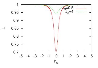
Figure 3: Variation of ground state $L$ with the staggered field $h_{s}$ for two different values of three spin interaction term with $N=10^{6}$, $t=100$ and $\delta=0.001$.

From Eq. (20), we find that the $L$ is unity deep inside the two antiferromagnetic phases where $2\eta_{k}$ is infinitesimally small for all $k$ and small $\delta$. The $L$ (or $L_{k}$) will start deviating from unity when the term $\sin^{2}(2\eta_{k})\sin^{2}(\Delta E_{k}t/2)$ picks up a non-zero value. It can be easily checked that $2\eta_{k}$ increases as $\Delta E_{k}$ approaches zero due to diverging $\tan\theta_{k}$ (see Eq. 11) at $h_{s}+\delta=0$, causing a dip in $L$ only at $h_{s}+\delta=0$. Thus, $L$ can neither detect AF to SLI phase transition discussed in section II which is captured by the fidelity, nor it can capture SLI to SLII phase transition. Unlike the models studied so far where the modes close to the critical mode contribute the most to the decay of the $L$, we will now show that it is not so in the present model. This is because the ground state for the critical mode $k=\pi$ at $h_{s}+\delta=0$ is $|\alpha_{k},\beta_{k}\rangle$, for which $L_{k=\pi}$ is unity. For the same reasons, the modes close to this critical mode also do not contribute to the decay of $L$. It is the other modes, away from the critical mode $k=\pi$ at $h_{s}+\delta=0$ satisfying $E_{+}(k)>0$ and $E_{-}(k)<0$ which actually influence the behavior of the $L$. This is one of the most interesting observations of the paper. Since the modes close to the critical mode are not involved in the dynamics, various power-law scalings of $L$, which are observed close to the QCP of other models quan06 , are not present in this model.

To understand why $L$ is not able to detect the various ground state phases generated due to the presence of $J_{3}$, let us revisit Eq. 8. As mentioned before, $|0,0\rangle$ and $|a_{k},b_{k}\rangle$ do not mix and we can concentrate on $|a_{k},0\rangle$ and $|0,b_{k}\rangle$ basis. In these two basis, $H_{k}$ can be written as

$$\frac{J_{3}}{2}\cos k\hat{I}+(h_{s}+\delta)\sigma^{z}-\cos(k/2)\sigma^{x}=\frac{J_{3}}{2}\cos k\hat{I}+H_{0}$$ (21)

where $\hat{I}$ is the $2\times 2$ identity matrix. The non-commutativity between the terms involving $\sigma^{x}$ and $\sigma^{z}$ causes the time evolution of the spin chain. On the other hand, the identity term in Eq. (21) only contributes to the phase of the evolving wave function and does not influence the $L$ which is a modulus-squared quantity. Hence, the dynamics is dominated by the minimum energy gap of the second part $H_{0}$ of the Hamiltonian chowdhury10 , which occurs at $h_{s}+\delta=0$; consequently, the $L$ shows a dip right here. Such an observation was also reported in the context of defect generation for a similar model where the staggered field is varied linearly as a function of time. The study finds that the scaling of the defect density is insensitive to the QPTs driven by the identity operator in the Hamiltonian chowdhury10 .

Since the $L$ usually shows a dip in the vicinity of a QCP, one refer to the staggered field $h_{s}+\delta=0$ as a dynamical critical point at which the energy gap vanishes for the dynamical critical mode $k_{c}^{d}=\pi$ and probe the scaling of the $L$ close to this dynamical critical point. We show below that the $L$ decays exponentially with the system size $N$ whereas it decays exponentially with $\delta^{2}$ for both the regions, $|h_{s}|>J_{3}/2$ and $|h_{s}|<J_{3}/2$ as shown in Fig. 4.

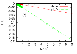
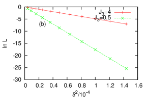
Figure 4: The exponential decrease of $L$ at $h_{s}+\delta=0$ with (a) system size $N$ for $t=0.1$ and $\delta=0.001$ and (b) with $\delta^{2}$ for $t=1$ and $N=10^{6}$.

To comprehend this behavior, let us concentrate on $S=$ln L which using Eq. (20) can be put in the form

$$S=\sum_{k}\ln\left(1-\sin^{2}2\eta_{k}\sin^{2}\frac{\Delta E_{k}t}{2}\right),$$ (22)

where the summation is only over the relevant $k-$modes satisfying $E_{-}(k)<0$ and $E_{+}(k)>0$. Since $\sin^{2}2\eta_{k}$ is the difference between two approximately equal angles in the limit $\delta\to 0$, it is very small as the dynamical critical mode and the near by modes do not appear in the summation. We therefore get a simplified expression

$$S \simeq -\sum_{k}4\eta_{k}^{2}\sin^{2}\left(\frac{\Delta E_{k}t}{2}\right)$$ (23)

$$\simeq -\sum_{k}\frac{\delta^{2}\sin^{2}(t\cos k/2)}{\cos^{2}(k/2)}$$

which explains the $\delta^{2}$ dependence of S or $\ln L$. It is difficult to estimate the system size dependence of the $L$ since the critical mode and the modes close to it do not contribute to the decay and hence no further simplifications can be done. However, one can focus on the modes closest to the dynamical critical mode $k_{c}^{d}=\pi$ for which $E_{-}(k)<0$ and $E_{+}(k)>0$ which contribute maximally to $L$. In the early time limit, one gets

$$S\simeq-\sum_{k}\delta^{2}t^{2}\propto-N$$

which is consistent with Fig. 4.

Our study shows that the $L$ is not able to detect the various phase transitions in the ground state phase diagram of the three spin interacting spin chain in presence of a staggered field. These transitions are generated due to the three spin interacting term $J_{3}$ which does not influence the dynamics of the Hamiltonian. The $L$ does not sense the presence of $J_{3}$ and detects only the QCPs corresponding to the case $J_{3}=0$ even when $J_{3}\neq 0$.

Although our study is restricted to a spin-1/2 model, the excitation spectrum as given in Eq. (21) may exist in other models also. For example, one may consider the Bose-Hubbard model in the hard core limit in the presence of a period two superlattice hen10 which has a rich phase diagram containing various phases like superfluid, Mott insulator, hole vacuum and particle vacuum phase. We expect similar results for the fidelity and the $L$ in this hard core boson model also .

At the end, we mention a couple of works which study the fidelity and $L$ of models containing multispin interactions in Ising type Hamiltonians liu12 ; lian11 . In ref. lian11, , the effect of some complicated three spin interaction on $L$ is studied and it was reported that a particular term of the Hamiltonian does not effect the position of the dip of the $L$ and modifies only the sharpness of the decay. On the other hand, we have studied here a completely different model with special types of QCPs and presented the appropriate arguments on why the $L$ is not able to detect the gapped to gapless phase transition points. At the same time, the physics of our model is very different from the model studied in Ref. lian11, due to the presence of staggered field which necessitates the introduction of two types of quasiparticles, thus making the problem very different from the models studied till now in the context of fidelity or Loschmidt echo.

V Conclusions

The ground state fidelity, or equivalently the ground state $L$ shows a dip at the quantum critical point and thus can in principle be used to determine the phase diagram of any model. We show that this is not always the case taking an example of a three spin interacting spin chain in presence of a stagerred field where the conventional method of divergence of stiffness constant could detect all the critical points but the method of fidelity and $L$ failed. While fidelity or fidelity susceptibility can capture the boundary between the gapped to gapless phase transition and is unable to detect the two Fermi points to four Fermi points phase transition within the gapless region, the Loschmidt echo shows a completely different picture. It is able to detect only one special point in the entire phase diagram and is not able to capture the critical points generated due to the presence of the three spin term. This is because the dynamics is entirely governed by the non-commuting terms of the reduced $2\times 2$ Hamiltonian in $k-$space and the identity matrix containing the three spin term only adds a phase to the wave function evolution. One of the interesting observations of this paper which has never been reported anywhere else to the best of our knowledge, is that the critical mode and its nearby modes do not contribute anything to the decay of Loschmidt echo. This is in contrast to the usual scenario where the modes around the critical modes contribute maximum. We would also like to point out here that in Ref. nofidelity, , it was shown that the fidelity susceptibility will not be able to detect any QPT if $\nu d>2$ which is not the case here.

Acknowledgements: UD acknowledges fruitful discussions with Shraddha Sharma and Tanay Nag, and thanks Amit Dutta for critically reading the manuscript.

References

- (1)
- (2) P. Zanardi and N. Paunkovic, Phys. Rev. E 74, 031123 (2006).
- (3) H-Q. Zhou and J. P. Barjaktarevic, J. Phys. A: Math. Theor. 41, 412001 (2008); H-Q. Zhou, R. Orus and G. Vidal, Phys. Rev. Lett. 100, 080601 (2008).
- (4) Shi-Jian Gu, Int. J. Mod. Phys. B 24, 4371 (2010).
- (5) P. D. Sacramento, N. Paunkovic and V. R. Vieira, Phys. Rev. A 84, 062318 (2011).
- (6) B. Damski, arxiv:1212.1528.
- (7) A. Dutta, , arXiv:1012.0653 (2010).
- (8) S. Sachdev, Quantum Phase Transitions(Cambridge University Press, Cambridge, England,1999).
- (9) B. K. Chakrabarti, A. Dutta and P. Sen, Quantum Ising Phases and transitions in transverse Ising Models, m41 (Springer, Heidelberg,1996).
- (10) Marek M Rams and B. Damksi, Phys. Rev. Lett 106, 055701 (2011); Marek M Rams and B Damski, Phys. Rev. A 84, 032324 (2011).
- (11) S. Yang, S. J. Gu, C. P. Sun and H-Q. Lin, Phys. Rev. A 78, 012304 (2008); J. H. Zhao and H. Q. Zhou, arxiv:0803.0814
- (12) P. Bounsante and A. Vezzani, Phys. Rev. Lett. 98, 110601 (2007).
- (13) D Schwandt, F. Alet and S. Capponi, Phys. Rev. Lett. 103, 170501 (2009);C. De Grandi, V. Gritsev and A. Polkovnikov, Phys. Rev. B 81, 012303 (2010); C. De Grandi, V. Gritsev and A. Polkovnikov, Phys. Rev. B 81, 224301 (2010).
- (14) M. Thakurathi, D. Sen and A. Dutta, Phys. Rev. B 86, 245424 (2012).
- (15) A. A. Patel, S. Sharma and A. Dutta, arxiv:1301.1930.
- (16) H. T. Quan, Z. Song, X. F. Liu, P. Zanardi and C. P Sun, Phys. Rev. Lett. 96, 140604 (2006).
- (17) F. M. Cucchietti, S. F. Vidal and J. P. Paz, Phys. Rev. A 75, 032337 (2007); D. Rossini, , Phys. Rev. A 75, 032333 (2007); L. Campos Venuti and P. Zanardi, Phys. Rev. A 81, 022113 (2010); L. Campos Venuti, N. T. Jacobson, S. Santra and P. Zanardi, Phys. Rev. Lett. 107, 010403 (2011).
- (18) V. Mukherjee, S. Sharma and A. Dutta, Phys. Rev. B 86, 020301 (2012).
- (19) A. Peres, Quantum Theory: Concepts and Methods (Kluwer Academic Publishers, Dordrecht); A. Peres, Phys. Rev. A 30, 1610 (1984).
- (20) R. A. Jalabert, and H. M. Pastawski, Phys. Rev. Lett. 86, 246 (2001)
- (21) Z. P. Karkuszewski, C. Jarzynski, and W. H. Zurek, Phys. Rev. Lett. 89, 170405 (2002)
- (22) N. R. Cerruti, S. Tomsovic, Phys. Rev. Lett. 88, 054103 (2002).
- (23) F. M. Cucchietti, , D.A. R. Dalvit, J.P. Paz, and W.H. Zurek, Phys. Rev. A 95, 105701 (2003).
- (24) Q. Zheng, W. G. Wang, X. P. Zhang and Z. Z. Ren, Phys. Lett. A 372, 5139 (2008); Q. Zheng, W. G. Wang, P. Q. Qin, P. Wang, X. P. Zhang and Z. Z. Ren, Phys. Rev. E 80, 016214 (2009).
- (25) J. F. Huan, Y. Li, J. Q. Liao. L. M. Kuang and C. P. Sun, Phys. Rev. A 80, 063829 (2009).
- (26) F. B. J. Buchkremer, R. Dumke, H. Levsen, G. Birkl and W. Ertmer, Phys. Rev. Lett. 85, 3121 (2000).
- (27) J. Zhang , Phys. Rev. A 80, 012305 (2009).
- (28) C. M. Sánchez, P. R. Levstein, R. H. Acosta and A. K. Chattah, Phys. Rev. A 80, 012328 (2009).
- (29) M. Roger, J. H. Hetherington and J. M. Delrieu, Rev. Mod. Phys. 55, 1 (1983).
- (30) I. Titvinidze and G. I. Japaridze, Eur. Phys. J. B 32, 383 (2003); A. A. Zvyagin and G. A. Skorobagatḱo, Phys. Rev. B 73, 024427 (2006).
- (31) Ping Lou, Wen-Chin Wu, and Ming-Che Chang, Phys. Rev. B 70, 064405 (2004); P. Lou, physica status solidi (b) 242, 3209 (2005).
- (32) P. Lou, physica status solidi (b) 241, 1343 (2004).
- (33) M. Topilko, T. Krokhmalskii, O. Derzhko and V. Ohanyan , Eur. Phys. J. B 85, 278 (2012);
- (34) T. Krokhmalskii, O. Derzhko, J. Stolze and T. Verkholyak, Phys. Rev. B 77, 174404 (2008);
- (35) D. Eloy and J. C. Xavier, Phys. Rev. B 86, 064421 (2012).
- (36) W.W. Cheng, C.J. Shan, Y.B. Sheng, L.Y. Gong and S.M. Zhao, Physica B 407 3671 (2012).
- (37) Zheng-Da Hu, Qi-Liang He and Jing-Bo Xu, Physica A: Stat. Mech. and its Applications 391, 6226 (2012).
- (38) Xiu-xing Zhang, Ai-ping Zhang and Fu-li Li, Phys. Lett. A 376, 2090 (2012).
- (39) H. L. Lian, Physica B 406, 4278 (2011).
- (40) H. L. Lian, D. P. Tian, Phys. Lett. A 375, 3604 (2011); X. Liu, M. Zhing, H. Xu and P. Tong, J. Stat. Mech: Thoery and Experiment, P01003 (2012).
- (41) E. Lieb, T. Schultz and D. Mattis, Ann. Phys.(N.Y.) 16 407 (1961).
- (42) J.E. Bunder and R. H. McKenzie, Phys. Rev. B., 60, 344, (1999).
- (43) O. Derzhko, T Krokhmalskii, J. Stolze and T. Verkholyak, Phys. Rev. B 79, 094410 (2009).
- (44) D. Chowdhury, U. Divakaran and A. Dutta, Phys. Rev. E. 81, 012101 (2010).
- (45) I Hen, M. Iskin and M. Rigol, Phys. Rev. B 81, 064503 (2010).