Improving Lower Bounds for the Quadratic Assignment Problem by applying a Distributed Dual Ascent Algorithm

Abstract

The application of the Reformulation Linearization Technique (RLT) to the Quadratic Assignment Problem (QAP) leads to a tight linear relaxation with huge dimensions that is hard to solve. Previous works found in the literature show that these relaxations combined with branch-and-bound algorithms belong to the state-of-the-art of exact methods for the QAP. For the level 3 RLT (RLT3), using this relaxation is prohibitive in conventional machines for instances with more than 22 locations due to memory limitations. This paper presents a distributed version of a dual ascent algorithm for the RLT3 QAP relaxation that approximately solves it for instances with up to 30 locations for the first time. Although, basically, the distributed algorithm has been implemented on top of its sequential conterpart, some changes, which improved not only the parallel performance but also the quality of solutions, were proposed here. When compared to other lower bounding methods found in the literature, our algorithm generates the best known lower bounds for 26 out of the 28 tested instances, reaching the optimal solution in 18 of them.

1 Introduction

Given $N$ objects, $N$ locations, a flow $f_{ik}$ from each object $i$ to each object $k$, $k\neq i$, and a distance $d_{jn}$ from each location $j$ to each location $n$, $n\neq j$, the quadratic assignment problem (QAP) consists of assigning each object $i$ to exactly a location $j$. We wish to find:

$$min\displaystyle\sum_{i=1}^{N}\sum_{j=1}^{N}\sum_{k=1\atop{k\not=i}}^{N}\sum_{n=1\atop{n\not=j}}^{N}f_{ik}d_{jn}x_{ij}x_{kn}:x\in X,\ x\in\left\{0,1\right\}\\$$ (1)

Initially presented by Koopmans & Beckmann (1957), the QAP has practical applications in several areas, such as facility layout, electronic circuit board design, construction planning, etc. The QAP is one of the most difficult and studied combinatorial optimization problems found in OR literature. Usually, difficult instances require a great deal of computational effort to be solved exactly. In Adams et al. (2007), for example, a 30-location instance is solved on a single cpu of a Dell 7150 PowerEdge server in 1,848 days. Thus, good lower bounds are crucial for solving instances with more than 15 locations in reasonable processing time. They would allow that a large number of alternative solutions is discarded during the search for the optimal solution in the branch-and-bound tree.

A summary of the techniques used for calculating lower bounds is presented in Loiola et al. (2007). In the QAPLIB website Burkard. et al. (1991), a table showing lower bounds for each instance of the site is presented. The best lower bounds were achieved by Burer & Vandenbussche (2006), Adams et al. (2007) and Hahn et al. (2012). The dual ascent algorithm based on the RLT3 formulation, described in Hahn et al. (2012), calculates tight lower bounds, but the use of such technique in conventional machines for instances with more than 25 locations is impossible due to its large memory requirements. For example, to solve an instance of 25 locations, Hahn, in Hahn et al. (2012), used a host with 173 GB of shared memory. Recently, a very difficult instance with 30 locations has been solved exactly also using the RLT3 formulation (see http://www.seas.upenn.edu/qaplib/news.html). In this case, the authors used the same cluster of machines, which contains hosts with up to 2 TB of shared memory.

The contribution of this paper is the proposal of a distributed application developed on top of the sequential algorithm proposed in Hahn et al. (2012), but not equivalent to it, since our new algorithm has some important changes, which improve not only the performance but also the quality of RLT3 lower bounds for some instances. This distributed algorithm executes on a conventional cluster of computers and generates the best known lower bounds for 26 out of the 28 tested instances, reaching the optimal solution in 18 of them.

2 Reformulation-linearization technique applied to the QAP

The reformulation-linearization technique was initially developed by Adams & Sherali (1986), aiming to generate tight linear programming relaxations for discrete and continuous nonconvex problems. For mixed zero-one programs involving $m$ binary variables, RLT establishes an $m$-level hierarchy of relaxations spanning from the ordinary linear programming relaxation to the convex hull of feasible integer solutions. For a given $z\in\{i,..,m\}$, the level-$z$ RLT, or RLT$z$, constructs various polynomial factors of degree $z$ consisting of the product of some $z$ binary variables $x_{j}$ or their complements $(1-x_{j})$. We find in the literature various RLT levels applied to the QAP, RLT1 in Hahn & Grant (1998), RLT2 in Adams et al. (2007) and RLT3 in Hahn et al. (2012). The RLT consists of two steps: the reformulation and linearization.

The RLT3 reformulation, presented in Hahn et al. (2012), consists of the following steps: (i) multiply each of $2N$ assignment constraints by each of the $N^{2}$ binary variables $x_{ij}$ (applying RLT1); (ii) multiply each of the $2N$ assignment constraints by each one of the $N^{2}(N-1)^{2}$ products $x_{ij}x_{kn}$, $k\not=i\$ and $\ n\not=j$ (applying RLT2); (iii) multiply each of the $2N$ assignment constraints by each one of the $N^{2}(N-1)^{2}(N-2)^{2}$ products $x_{ij}x_{kn}x_{pq}$, $p\not=k\not=i\$ and $q\not=n\not=j$ (applying RLT3). Moreover, remove the products $x_{ij}x_{kn}$ if $(k=i\$and$\ n\not=j)\$or$\ (k\not=i\$and$\ n=j)$ in quadratic expressions; remove all products $x_{ij}x_{kn}x_{pq}$ if $(p=i\$and$\ q\not=j),\ (p=k\$ and $\ q\not=n),\ (p\not=i\$and$\ q=j)$ or $(p\not=k\$and$\ q=n)$ in cubic expressions; and, finally, remove all products $x_{ij}x_{kn}x_{pq}x_{gh}$ if $(g=i\$and$\ h\not=j),\ (g=k\$and$\ h\not=n),\ (g=p\$and$\ h\not=q),\ (g\not=i\$and$\ h=j),\ (g\not=k\$and$\ h=n)\$ or $\ (g\not=p\$and$\ h=q)$ in biquadratic expressions.

The linearization consists of: (i) replace each product $x_{ij}x_{kn}$, with $i\not=k$ and $j\not=n$, by the continuous variable $y_{ijkn}$, imposing the constraints $y_{ijkn}=y_{knij}$ (2 complementaries) for all $(i,j,k,n)$ with $i<k$ and $j\not=n$ (applying RLT1); (ii) replace each product $x_{ij}x_{kn}x_{pq}$, with $i\not=k\not=p$ and $j\not=n\not=q$, by the continuous variable $z_{ijknpq}$, imposing the constraints $z_{ijknpq}=z_{ijpqkn}=z_{knijpq}=z_{knpqij}=z_{pqijkn}=z_{pqknij}$ (6 complementaries) for all $(i,j,k,n,p,q)$ with $i<k<p$ and $j\not=n\not=q$ (applying RLT2); (iii) replace each product $x_{ij}x_{kn}x_{pq}x_{gh}$ for $v_{ijknpqgh}$, with $i\not=k\not=p\not=g$ and $j\not=n\not=q\not=h$, by the continuous variable $v_{ijknpqgh}$, imposing the constraints $v_{ijknpqgh}=v_{ijknghpq}=...=v_{ghpqknij}$ (24 complementaries) for all $(i,j,k,n,p,q,g,h)$ with $i<k<p<g$ and $j\not=n\not=q\not=h$ (applying RLT3).

At the end of RLT3 reformulation, we achieve the following objective function:

$$min\left\{\displaystyle\sum_{i=1}^{N}\sum_{j=1}^{N}B_{ij}x_{ij}+\sum_{i=1}^{N}\sum_{j=1}^{N}\sum_{k=1\atop{k\not=i}}^{N}\sum_{n=1\atop{n\not=j}}^{N}C_{ijkn}y_{ijkn}+\displaystyle\sum_{i=1}^{N}\sum_{j=1}^{N}\sum_{k=1\atop{k\not=i}}^{N}\sum_{n=1\atop{n\not=j}}^{N}\sum_{p=1\atop{p\not=i,k}}^{N}\sum_{q=1\atop{q\not=j,n}}^{N}D_{ijknpq}z_{ijknpq}\atop{\displaystyle+\sum_{i=1}^{N}\sum_{j=1}^{N}\sum_{k=1\atop{k\not=i}}^{N}\sum_{n=1\atop{n\not=j}}^{N}\sum_{p=1\atop{p\not=i,k}}^{N}\sum_{q=1\atop{q\not=j,n}}^{N}\sum_{g=1\atop{g\not=i,k,p}}^{N}\sum_{h=1\atop{h\not=j,n,q}}^{N}E_{ijknpqgh}v_{ijknpqgh}+LB}\right\}$$ (2)

In the objective function (2), consider the constant term $LB=0$, each coefficient $B_{ij}=0\ \forall\ (i,j)$, each coefficient $C_{ijkn}=f_{ik}\times d_{jn}\ \forall\ (i,j,k,n)\$ with $\ i\not=k$ and $j\not=n$, each coefficient $D_{ijknpq}=0\ \forall\ (i,j,k,n,p,q)\$ with $\ i\not=k\not=p$ and $j\not=n\not=q\$, each coefficient $E_{ijknpqgh}=0\ \forall\ (i,j,k,n,p,q,g,h)\$ with $\ i\not=k\not=p\not=g$ and $j\not=n\not=q\not=h$.

The dual ascent algorithm proposed in Hahn et al. (2012) consists of updating the constant term $LB$ and the cost matrices $B$, $C$, $D$ and $E$ in such a way that the cost of any (integer) feasible solution with respect to the modified objective function remains unchanged, while maintaining nonnegative coefficients. As a consequence of this property, the value of $LB$ at any moment of the execution is a valid lower bound on the optimal solution cost for the QAP. In the light of these aspects, the following procedures are developed:

1. Cost spreading: consists of the cost distributions from matrix $B$ to $C$, from matrix $C$ to $D$ and from matrix $D$ to $E$. In the cost spreading procedure from matrix $B$ to $C$, for each $(i,j)$, the coefficient $B_{ij}$ is spread through $(N-1)$ rows of matrix $C$, i.e., each element $C_{ijkn}$ is added by $B_{ij}\ /\ (N-1)$, $\forall\ k\not=i\$ and $\ n\not=j$. After such updating, $B_{ij}$ is updated to $0$ for each $(i,j)$. The same procedure is repeated from matrix $C$ to $D$, where each coefficient $C_{ijkn}$ is spread through $(N-2)$ rows of matrix $D$, and from matrix $D$ to $E$, where each coefficient $D_{ijknpq}$ is spread through $(N-3)$ rows of matrix $E$.

2. Cost concentration: in this procedure we used the Hungarian Algorithm, Munkres (1957), to concentrate the costs from matrix $E$ to $D$, from matrix $D$ to $C$, from matrix $C$ to $B$ and from matrix $B$ to $LB$. The cost concentrations from matrix $E$ to $D$ are represented as $D_{ijknpq}$ $\leftarrow Hungarian(E_{ijknpq})$. This procedure uses a matrix $M$ with size $(N-3)^{2}$ to receive the $(N-3)^{2}$ coefficients of the submatrix $E_{ijknpq}$: for each $(r,s=1,..,N-3)$, $M_{rs}$ receives $E_{ijknpqgh}$, where $g$ ($h$) is the $r$-th row ($s$-th column) different from $i,k,p$ ($j,n,q$) in the submatrix $E_{ijknpq}$. Then, the Hungarian algorithm is applied to $M$ to obtain the total cost to be added to $D_{ijknpq}$, and the coefficients of the submatrix $E_{ijknpq}$ are replaced by the corresponding residual coefficients from $M$. The same procedure is repeated as $C_{ijkn}$ $\leftarrow Hungarian(D_{ijkn})$, $B_{ij}$ $\leftarrow Hungarian(C_{ij})$ and $LB\leftarrow Hungarian(B)$. In these procedures, the sizes of $M$ are $(N-2)^{2}$, $(N-1)^{2}$ and $N^{2}$, respectively.

3. Costs transfer between complementary coefficients: Differently from Hahn et al. (2012), the cost transfers always replace each coefficient by the arithmetic mean of all its complementaries. It is applied as follows: (i) In the matrix $C$, for each $(i,j,k,n)$, $C_{ijkn}\leftarrow$ $C_{knij}\leftarrow$ $(C_{ijkn}+C_{knij})/2$, with $i<k\$ and $j\not=n$; (ii) In the matrix $D$, for each $(i,j,k,n,p,q)$, $D_{ijknpq}\leftarrow$ $D_{ijpqkn}\leftarrow$ $D_{knijpq}\leftarrow$ $D_{knpqij}\leftarrow$ $D_{pqijkn}\leftarrow$ $D_{pqknij}=(D_{ijknpq}+$ $D_{ijpqkn}+$ $D_{knijpq}+$ $D_{knpqij}+$ $D_{pqijkn}+$ $D_{pqknij})/6$, with $i<k<p\$ and $\ j\not=n\not=q$; (iii) In the matrix $E$, for each $(i,j,k,n,p,q,g,h)$, $E_{ijknpqgh}$ $\leftarrow$ $E_{ijknghpq}$ $\leftarrow$ … $\leftarrow$ $E_{ghpqknij}$ $\leftarrow$ $(E_{ijknpqgh}+E_{ijknghpq}+\ ...\ +E_{ghpqknij})/24$, with $i<k<p<g\$ and $\ j\not=n\not=q\not=h$.

3 Distributed Algorithm

In our distributed version, consider $T$ the set of hosts running the application, and let $R_{t}\ (R_{t}\in T)$ be the identification of a host. Let $f_{ik}$ and $d_{jn}$ be flow and distance matrices respectively, according to equation (1), $LB$, the lower bound, and $B$,$C$,$D$ and $E$, the matrices presented in the objective function (2). Consider $G_{ij}$ as a set composed of submatrices $B$, $C$, $D$, $E$ with the same $(i,j)$ stored and processed on $R_{t}$. Sets of $G$ are evenly distributed among the hosts. See Figure 1 for an example with twenty hosts, running an instance of $N=20$. In this figure, the set $G_{15,7}$ composed of submatrices $B_{15,7}$, $C_{15,7,k,n}$, $D_{15,7,k,n,p,q}$ and $E_{15,7,k,n,p,q,g,h}$ is stored and processed on the host $R_{13}$. Other forms of mapping can be accomplished, since $G_{ij}$ is used as a load distribution unit.

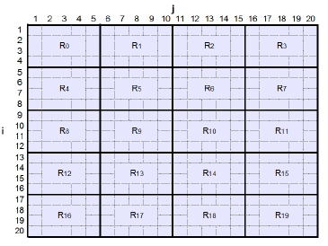
Figure 1: Example of allocation of sets $G_{ij}$ on 20 hosts

The RLT3 algorithm applied to the QAP requires a lot of RAM memory to store the coefficients of the matrices. An instance with $N=30$, for example, requires around 1.6 TByte to store the matrix $E$, which is composed of $N^{2}$ x $(N-1)^{2}$ x $(N-2)^{2}$ x $(N-3)^{2}$ elements, each one keeping an integer or float data (4 bytes). Although some improvements have been proposed in Hahn et al. (2012), the required memory goes on being much bigger than the provided by modern computers.

In the distributed algorithm, complementaries belonging to different sets can be allocated on different hosts, requiring that hosts communicate among themselves during their executions. The distributed algorithm runs several iterations and at each of them, four steps are executed. In the first one, complementary costs of matrix $E$ are exchanged. Complementary costs stored in $R_{x}$, needed in $R_{z}$, are transferred through messages from $R_{x}$ to $R_{z}$, denoted as $Comp(E)_{xz}$. In the next two steps, complementary costs of matrices $D$ and $C$, are sent through $Comp(D)_{xz}\ and\ Comp(C)_{xz}$ messages, respectively. In the final stage, matrices $B$ are transmitted through $Mens(B)_{xz}$ messages. In small instances, up to $N=12$, communication overhead does not impact the performance negatively. However, in bigger instances, the communication of complementary costs of matrix E can represent up to 70% of the total execution time in instances with $N=30$.

The steps of the distributed algorithm executed in the process $R_{t}$ are described next.

1- Initialization: $LB\leftarrow 0$, $B_{ij}\leftarrow 0\ \forall\ (i,j)$, $C_{ijkn}\leftarrow$ $f_{ik}\times d_{jn}$ $\ \forall\ (i,j,k,n)$ with $i\not=k\$ and $\ j\not=n$, $D_{ijknpq}\leftarrow 0$ $\ \forall\ (i,j,k,n,p,q)$ with $i\not=k\not=p\$ and $\ j\not=n\not=q$, $E_{ijknpqgh}\leftarrow 0$ $\ \forall\ (i,j,k,n,p,q,g,h)$ with $i\not=k\not=p\not=g$ and $j\not=n\not=q\not=h$, $\ cont\leftarrow 1$, $\ lim\leftarrow$ total of iterations and $optimal\leftarrow$ optimal solution or best known solution cost.

2 - Transferring complementaries of matrix $C$: For each $R_{s}\in T\$ and $\ R_{s}\not=R_{t}$, and for each $(i,j,k,n)\ |\ G_{ij}$ allocated in $R_{t}\ and\ G_{kn}$ allocated in $R_{s},\ i<k\$ and $\ j\not=n$, store coefficients $C_{ijkn}$ in $Comp(C)_{ts}$ $\ \forall\ i<k\$ and $\ j\not=n$. Send $Comp(C)_{ts}$ to $R_{s}$. Upon receiving messages from other hosts, for each $G_{ij}$ allocated in $R_{t}$, $C_{ijkn}\leftarrow(C_{ijkn}+C_{knij})/2$.

3 - Cost concentration from matrix $C$ to matrix $B$: For each $G_{ij}$ allocated in $R_{t}$, concentrate the coefficients from matrix  $C$  to  $B$,  by executing the  Hungarian  Algorithm,   $B_{ij}$ $\leftarrow Hungarian(C_{ij})$.

4- Transferring matrix $B$: For each $(i,j)\ |\ G_{ij}$ allocated in $R_{t}$, store coefficients $B_{ij}$ in $Mens(B)$. Broadcast $Mens(B)$ to all hosts. After receiving messages from all other hosts, update local matrix $B$.

5- Cost concentration from matrix $B$ to $LB$: $LB\leftarrow Hungarian(B)$.

6 - Loop: Repeat until $cont=lim$ or $LB=optimal$, The loop termination condition is achieved when the total number of iterations reaches the previously defined limit ($cont=lim$) or the optimal solution is equal to the current lower bound ($LB=optimal$).

7 - Cost spreading from matrix $B$ to $C$: For each $(i,j)\ |\ G_{ij}$ allocated in $R_{t}$, spread $B_{ij}$ through $(N-1)$ submatrix rows of $C_{ij}$. Each cost element $C_{ijkn}$ is increased by $B_{ij}\ /\ (N-1)$ $\forall\ k\not=i\ e\ j\not=n$.

8 - Cost spreading from matrix $C$ to $D$: For each $(i,j,k,n)\ |\ G_{ij}$ allocated in $R_{t}$ and $i\not=k\$ and $\ j\not=n$, spread $C_{ijkn}$ through $(N-2)$ submatrix rows of $D_{ijkn}$. Each cost element $D_{ijknpq}$ is increased by $C_{ijkn}\ /\ (N-2)$ $\forall\ p\not=i,k\$ and $\ q\not=j,n$.

9 - Cost spreading from matrix $D$ to $E$: For each $(i,j,k,n,p,q)\ |\ G_{ij}$ allocated in $R_{t}$ and $i\not=k,p\$ and $\ j\not=n,q$, spread $D_{ijknpq}$ through $(N-3)$ submatrix rows of $E_{ijknpq}$. Each cost element $E_{ijknpqgh}$ is increased by $D_{ijknpq}\ /\ (N-3)\ \forall\ g\not=i,k,p\$ and $\ h\not=j,n,q$.

10 - Cost transfer between complementary coefficients of matrix $E$: For each $R_{s}\in T\$ and $\ R_{s}\not=R_{t}$, for each $(i,j,k,n,p,q,g,h)\ |\ G_{ij}$ allocated in $R_{t}\$ and $\ (G_{kn},G_{pq}$ or $G_{gh})$ allocated in $R_{s}$ and $i<k<p<g\$ and $\ j\not=n\not=q\not=h$, include the coefficients $E_{ijknpqgh}$ in $Comp(E)_{ts}$. Send message containing $Comp(E)_{ts}$. Upon receiving messages from all hosts, for each $(i,j,k,n,p,q,g,h)\ |\ G_{ij}$ allocated in $R_{t}$, $E_{ijknpqgh}\leftarrow E_{ijknghpq}\leftarrow E_{ijpqkngh}\leftarrow E_{ijpqghkn}\leftarrow E_{ijghknpq}\leftarrow E_{ijghpqkn}\leftarrow(E_{ijknpqgh}+E_{ijknghpq}+\ ...\ +E_{ghpqknij})/24$.

11 - Cost concentration from matrix $E$ to $D$: For each $(i,j,k,n,p,q)\ |\ G_{ij}$ allocated in $R_{t}$, concentrate the submatrices from $E$ to $D$, i.e., $D_{ijknpq}$ $\leftarrow Hungarian(E_{ijknpq})$.

12 - Cost transfer between complementary coefficients of matrix $D$: For each $R_{s}\in T\$ and $\ R_{s}\not=R_{t}$, for each $(i,j,k,n,p,q)\ |\ G_{ij}$ allocated in $R_{r}\$ and $\ (G_{kn}$ or $G_{pq})$ allocated in $R_{s}\$ and $\ i<k<p\$ and $\ j\not=n\not=q,$ include the coefficients $D_{ijknpq}$ in $Comp(D)_{ts}$. Send message containing $Comp(D)_{ts}$. Upon receiving messages from all hosts, for each $(i,j,k,n,p,q)\ |\ G_{ij}\in R_{t}$, $D_{ijknpq}\leftarrow D_{ijpqkn}\leftarrow(D_{ijknpq}+D_{ijpqkn}+D_{knijpq}+D_{knpqij}+D_{pqijkn}+D_{pqknij})/6$.

13 - Cost concentration from matrix $D$ to $C$: For each $(i,j,k,n)\ |\ G_{ij}$ allocated in $R_{t}$, concentrate the submatrices from $D$ to $C$, i.e. , $C_{ijkn}$ $\leftarrow Hungarian(D_{ijkn})$.

14, 15, 16, and 17 - These steps are identical to Steps 2, 3, 4, and 5, respectively.

18 - loop end: Increase the variable $cont$ and return to Step 6.

Compared to the sequential version, the following modifications have been applied in the distributed algorithm: (i) use of floating point numbers instead of integers for cost coefficients; (ii) use of arithmetic means to transfer costs among complementary coefficients; (iii) execution of all cost transfers among complementary coefficients before concentration; and (iv) never spreading from $LB$ to matrix $B$.

From all these differences, the most important one is that of item (ii). In the sequential dual ascent algorithm proposed in Hahn et al. (2012), cost transfers are performed with the aim of increasing all cost coefficients of the current submatrix $M$, by pushing residual cost from its complementaries, before applying the cost concentration in that matrix. This approach imposes a sequential handling of submatrices at the same RLT level. Taking arithmetic means allow that such matrices are processed in parallel but prevents from using residual costs resulting from the Hungarian algorithm in other matrices at the same RLT level in the same iteration. This reuse of costs is not possible because all costs are evenly distributed among all complementaries before all cost concentrations are performed at that level. Initially, we expected that such modification would significantly slow down the convergence of the lower bound and/or substantially reduce its quality but the experiments reported in the next section show that neither effects are observed. In fact, we obtained better lower bounds in some cases.

4 Experimental Results

Table 1: Comparison between the newly proposed distributed algorithm and other techniques

					Distributed
Instance	Optimal	BV04	HH01	HZ07	Version
					$LB$	gap	time(s)	Speedup	hosts	iterations
had14	2724	0.00%*	-	-	2724	0.00% *	559	1.62	4	29
had16	3720	0.13%	0.00% *	0.02%	3720	0.00% *	744	5.83	8	22
had18	5358	0.11%	0.00% *	0.02%	5358	0.00% *	5456	5.27	9	59
had20	6922	0.16%	0.00% *	0.03%	6922	0.00% *	16118	NA	16	109
kra30a	88900	2.50%	2,98%	-	88424	0.54%	196835	NA	90	162
nug12	578	1.73%	0.00% *	0.14%	578	0.00% *	73	2.75	4	16
nug15	1150	0.78%	0.00% *	0.08%	1150	0.00% *	360	5.28	9	22
nug16a	1610	0.75%	-	-	1610	0.00% *	1132	5.73	8	34
nug16b	1240	1.69%	-	-	1240	0.00% *	1294	5.71	8	39
nug18	1930	1.92%	-	0.00% *	1930	0.00% *	7172	5.36	9	78
nug20	2570	2.49%	2.41%	0.14%	2570	0.00% *	30129	NA	20	249
nug22	3596	2.34%	2.36%	0.08%	3596	0.00% *	41616	NA	22	157
nug24	3488	2.61%	-	-	3478	0.28%	173520	NA	24	300
nug25	3744	3.29%	-	-	3689	1.44%	172020	NA	25	211
nug28	5166	2.92%	-	-	5038	2.48%	171783	NA	49	118
nug30	6124	3.10%	5.78%	-	5940	3.00%	229583	NA	100	119
rou15	354210	1.13%	0.00% *	0.00% *	354210	0.00% *	323	5.78	9	20
rou20	725520	4.19%	3.60%	0.03%	720137	0.74%	37079	NA	25	300
tai15a	388214	2.86%	-	-	388214	0.00% *	737	6.18	9	46
tai17a	491812	3.11%	-	-	491812	0.00% *	1259	13.18	17	46
tai20a	703482	4.52%	3.93%	703482 *	698271	0.74%	45720	NA	25	300
tai25a	1167256	4.66%	6.48%	-	1122200	3.87%	101170	NA	25	124
tai30a	1818146	6.12%	7.25%	-	1724510	5.15%	112085	NA	100	58
tho30	149936	4.75%	9.82%	-	142990	4.63%	145713	NA	100	79
chr18a	11098	0.00% *	-	-	11098	0.00% *	1892	5.32	9	20
chr20a	2192	0.18%	-	-	2192	0.00% *	5914	NA	16	39
chr20b	2298	0.13%	-	-	2298	0.00% *	3708	NA	16	24
chr22a	6156	0.03%	-	-	6156	0.00% *	5321	NA	22	20

The application was implemented using the programming language C++ with the library IntelMPI library. The experiments were performed in the Netuno Cluster, see Silva et al. (2011), a cluster composed of 256 hosts, interconnected by infiniband. Each host consists of a two Intel Xeon E5430 2.66GHz Quad core processor with 12MB cache L2 and 16 GB of RAM per host.

A unique process is executed per host, allowing that it uses the total available memory without resource contention usually caused by process concurrency. So, only one core per host is used to execute the application.

For evaluation of the proposed distributed algorithm, the application terminates when the optimal solution is found or when a total of 300 iterations is executed, respecting a time limit (usually about three days per instance) that varies according the machine availability in the cluster.

Table 1 presents the results for different instances and sizes from the QAPLIB. In the first column of Table 1, there are the instance names and the corresponding dimensions. For example, nug20 represents an instance nug, from Nugent et al. (1968), with size $N=20$. In the second column, there are the optimal values for each instance. The third column (BV04) contains the gaps obtained by the lift-and-project relaxation proposed in Burer & Vandenbussche (2006). At the fourth column (HH01), one finds the gaps obtained by the RLT2 based dual ascent algorithm proposed in Adams et al. (2007). In the fifth column (HZ07), there are the gaps obtained by the RLT3 based dual ascent algorithm proposed in Hahn et al. (2012). The results presented for the last two methods were obtained from the QAPLIB website, which does not contain values for all instances. In the sixth column, we show the lower bounds obtained in the RLT3 distributed version proposed in this paper. In the seventh column, we present the corresponding gaps, in the eighth column, the execution times in seconds, and in the last three columns, the speedups obtained via parallelism, the number of hosts used, and the number of iterations performed.

Also in Table 1, notice that the lower bounds that correspond to optimal solution costs or gaps that are zero are marked with an asterisk, and those which are the best known gaps are in bold printed. For some instances, it was not possible to execute the sequential versions because of the memory constraints, in those cases the calculation of speedups were not applicable, as indicated in the table (NA).

5 Conclusion

The distributed version achieved goods results compared with other proposals, reaching the best known bounds of 26 out of 28 instances, being 18 of them the optimal solutions. The distributed algorithm allowed the execution of instances with size $N=28$ and $N=30$ for the first time using RLT3. Those good results were achieved due to the use some of parallelism and the changes proposed in the original sequential code.

References

- Adams et al. (2007) Adams, W. P., Guignard, M., Hahn, P. M., & Hightower, W. L. (2007). A level-2 reformulation-linearization technique bound for the quadratic assignment problem. European Journal of Operational Research, 180, 983–996.
- Adams & Sherali (1986) Adams, W. P., & Sherali, H. D. (1986). A tight linearization and an algorithm for zero-one quadratic programming problems. Manage. Sci., 32, 1274–1290.
- Burer & Vandenbussche (2006) Burer, S., & Vandenbussche, D. (2006). Solving lift-and-project relaxations of binary integer programs. SIAM Journal on Optimization, 16, 726–750.
- Burkard. et al. (1991) Burkard., R. E., Karisch., S. E., & Rendl, F. (1991). Qaplib – a quadratic assignment problem library. European Journal of Operational Research, 55, 115–119.
- Hahn & Grant (1998) Hahn, P. M., & Grant, T. (1998). Lower bounds for the quadratic assignment problem based upon a dual formulation. Operations Research, 46, 912–922.
- Hahn et al. (2012) Hahn, P. M., Zhu, Y.-R., Guignard, M., Higthower, W. L., & Saltzman, M. (2012). A level-3 reformulation-linearization technique-based bound for the quadratic assignment problem. INFORMS Journal on Computing, 24, 202–209.
- Koopmans & Beckmann (1957) Koopmans, T. C., & Beckmann, M. (1957). Assignment problems and the location of economic activities. Econometrica, 25, 53–76.
- Loiola et al. (2007) Loiola, E. M., de Abreu, N. M. M., Boaventura-Netto, P. O., Hahn, P. M., & Querido, T. (2007). A survey for the quadratic assignment problem. European Journal of Operational Research, 176, 657–690.
- Munkres (1957) Munkres, J. (1957). Algorithms for the assignment and transportation problems. Journal of the Society of Industrial and Applied Mathematics, 5, 32–38.
- Nugent et al. (1968) Nugent, C. E., Vollmann, T. E., & Ruml, J. (1968). An experimental comparison of techniques for the assignment of facilities to locations. Operations Research, 16, 150–173.
- Silva et al. (2011) Silva, G. P., Correa, J., Bentes, C., Guedes, S., & Gabioux, M. (2011). The experience in designing and building the high performance cluster netuno. Computer Architecture and High Performance Computing, Symposium on, 0, 144–151.