Numerical Approaches on Driven Elastic Interfaces in Random Media

Abstract

We discuss the universal dynamics of elastic interfaces in quenched random media. We focus in the relation between the rough geometry and collective transport properties in driven steady-states. Specially devised numerical algorithms allow us to analyze the equilibrium, creep, and depinning regimes of motion in minimal models. The relevance of our results for understanding domain wall experiments is outlined. To cite this article: E. E. Ferrero, S. Bustingorry, A. B. Kolton, A. Rosso, C.R. Physique XX (XXXX).

Résumé Approches Numériques pour les interfaces élastiques en milieu aléatoire Nous discutons les principaux résultats obtenus sur les proprietés universelles de la dynamique des interfaces élastiques en milieu aléatoire. Une attention particulière sera dediée à la relation entre la géometrie rugueuse de l’interface en mouvement et ses propietés de transport collectif. Les approches numériques développées permettent de décrire les proprietés d’équilibre, la dynamique de creep et la transition de dépiégeage de l’interface. Nous discutons aussi la pertinence de nos résultats dans les expériences sur la dynamique des parois.

Pour citer cet article : E. E. Ferrero, S. Bustingorry, A. B. Kolton, A. Rosso, C.R. Physique XX (XXXX).

Physics

, , ,

Received *****; accepted after revision +++++

1 Introduction

The out of equilibrium interplay between quenched disorder and elasticity in uniformly driven interfaces is at the root of the universal dynamical response displayed by very diverse physical systems. Examples are magnetic [1, 2, 3, 4, 5] or ferroelectric domain walls [6, 7, 8, 9, 10], contact lines in wetting [11, 12], fractures [13, 14], and earthquakes [15]. In this paper we discuss the basic phenomenology that emerges by solving, with specially devised numerical methods, the minimal models proposed for capturing such dynamical behavior.

Universal dynamical properties can be captured, both qualitatively and quantitatively, by rather simple models. To be concrete we will focus on the paradigmatic driven quenched-Edwards-Wilkinson (QEW) universality class, minimally described by

$$\gamma\partial_{t}u(x,t)=c\partial_{x}^{2}u(x,t)+F_{p}(u,x)+f+\eta(x,t).$$ (1)

This equation models the overdamped dynamics of an elastic interface with a univalued scalar displacement field $u(x,t)$, with $x$ a vector of dimension $d$, such that the interface is embedded in a space of dimension $D=d+1$. The elastic approximation made above, assumes small deformations such that the elastic part of the energy is well described by $H_{el}=(c/2)\int_{x}dx^{d}[\nabla u]^{2}$. We are thus ignoring “plastic” deformations such as overhangs or pinched-off loops that might appear in real interfaces, and assuming that elastic interactions are short-ranged, with a stiffness constant $c$. The contact with a thermal bath at temperature $T$ is modeled by a Langevin noise, such that $\langle\eta(x,t)\eta(x^{\prime},t^{\prime})\rangle=2k_{B}T\gamma\delta(x-x^{\prime})\delta(t-t^{\prime})$. Finally, the interface is coupled to a uniform driving force $f$ and to a quenched pinning force $F_{p}$, which arises from the disorder in the host materials. We will consider a non-biased pinning force characterized by its disorder-averaged correlator

$$\overline{F_{p}(u,x)F_{p}(u^{\prime},x^{\prime})}=\Delta(u-u^{\prime})\delta(x-x^{\prime}),$$ (2)

with $\Delta(x)$ a short-ranged function, of range $r_{f}$ (determined by the domain wall width in real interfaces with point disorder). For the so-called random bond (RB) case, the elastic line moves in a random short-range correlated potential. The corresponding pinning force is $F_{p}(u,x)=-\partial_{u}U(u,x)$, where $U(u,x)$ is the random potential, and thus $\int_{u}\Delta(u,x)=0$. For the random field (RF) case, $U(u,x)$ is a random walk as a function of $u$, with diffusion constant $\int_{u}\Delta(u,x)>0$ [16].

The model just defined is minimal, and in order to compare with experiments other ingredients might be considered. For example in charge density waves and vortices, the elastic structure is periodic [17, 18], while in fracture [14, 19, 20, 21, 22] and wetting [23, 24] the elastic interactions are long ranged. Moreover, anharmonic corrections to the elasticity or anisotropies can be also relevant [25, 26]. Remarkably, all these different universality classes (with different critical exponents) share the same basic physics of the QEW model discussed in the following sections.

2 Transport and Geometry of Driven Interfaces in Random Media

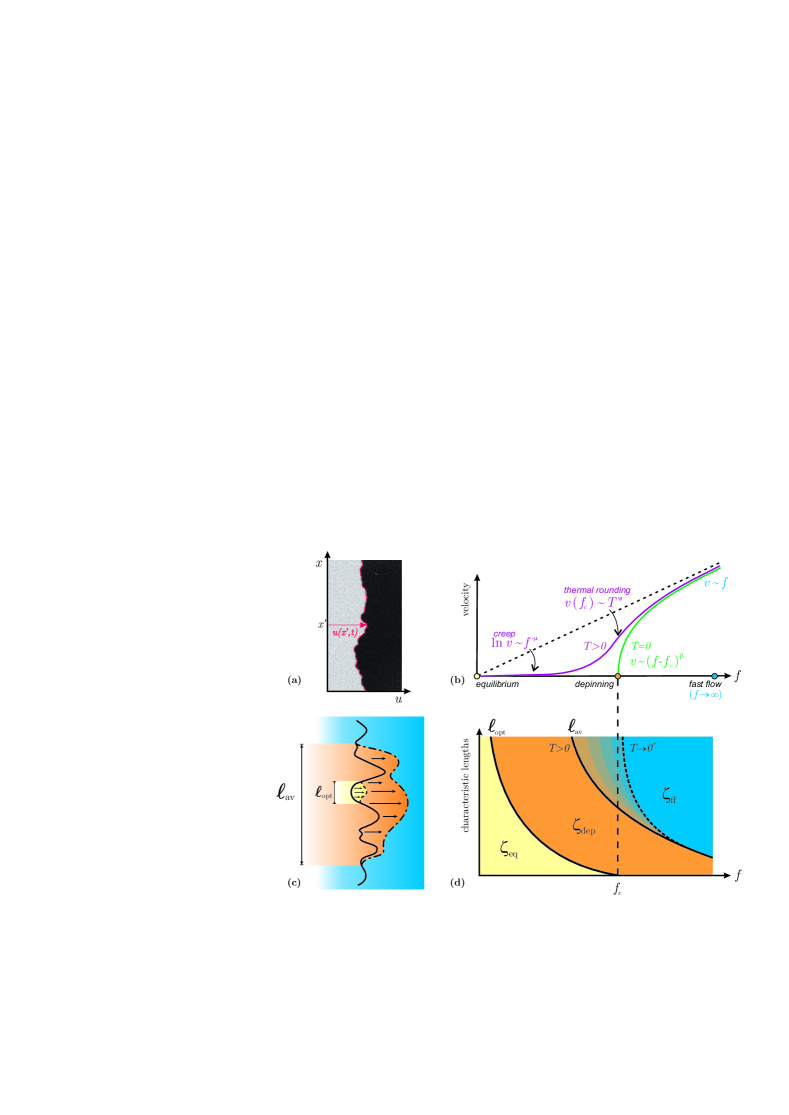
Figure 1: Linking transport and geometry. (a) Snapshot of a domain wall in a two dimensional ferromagnet [27]. (b) Typical velocity-force characteristics. (c) Crossover lengths ${{\ell}_{\tt opt}}$ and ${{\ell}_{\tt av}}$ representing the optimal excitation and the deterministic avalanches, respectively. (d) Geometric crossover diagram.

Disorder makes the interface dynamics very rich. On one side, the interface appears rough, both in absence and in presence of drive. On the other side, the response of the system to a finite drive is strongly nonlinear and, at zero temperature, motion exists only above a finite threshold, the so-called critical force $f_{c}$. As summarized in  Fig. 1 collective dynamics is observed in different regimes: just above $f_{c}$ the motion is very jerky, and displays collective rearrangements or avalanches of a typical size ${{\ell}_{\tt av}}$. Below $f_{c}$ motion is possible only by thermal activation over energy barriers and the interface slowly fluctuates backward and forward. This “futile” and reversible dynamics takes place up to a characteristic size ${{\ell}_{\tt opt}}$ above which energy barriers do not exist before the next lower-energy metastable state and the interface moves only forward pulled by the finite drive $f$. As $f\to 0$ both ${{\ell}_{\tt opt}}$ and the energy barriers diverge.

2.1 Three reference stationary states

Universality manifests, both in the transport and in the geometry of the moving interface, through the existence of robust critical exponents. These describe the rate of power-law divergences of important quantities as the control parameter $f$ approaches three special states: (i) the equilibrium ($f=0$); (ii) the depinning ($f=f_{c}$, $T=0$), and the fast-flow ($f\gg f_{c}$). Beyond some microscopic length-scale [28, 29] these three steady-states have the peculiarity that the geometry is self-affine with their characteristic roughness exponent: (i) ${\zeta_{\tt eq}}$, (ii) ${\zeta_{\tt dep}}$, and (iii) ${\zeta_{\tt ff}}$. Self-affinity means that length $x$ and displacement $u$ can be rescaled as $x^{\prime}=ax$ and $u^{\prime}=a^{-\zeta}u$ into a new interface $u^{\prime}(x^{\prime})$ which is statistically equivalent to $u(x)$, namely $u(ax)\sim a^{\zeta}u(x)$. Transport properties in these three points are very different: At equilibrium, the mean velocity is zero and the dynamics is glassy: at small length scales, we observe a fast futile motion, while in order to observe a rearrangement on a large scale size $l$ we need to overcome a barrier $E_{b}(l)$ growing as $E_{b}\sim l^{\theta}$, with $\theta$ a positive and universal exponent. Dimensional analysis suggests that $\theta=d-2+2{\zeta_{\tt eq}}$, which is confirmed by accurate numerical studies [30]. At the zero temperature depinning transition the velocity vanishes as $v(f,T=0)\sim(f-f_{c})^{\beta}$ for $f>f_{c}$ while $v=0$ for $f<f_{c}$. At finite temperature, this sharp transition is rounded and the velocity behaves as $v(f_{c},T)\sim T^{\psi}$. This is the so-called thermal rounding regime. At large force, $f\gg f_{c}$, in the fast-flow regime, we recover the linear response $v\sim f$. Here impurities generate an effective thermal noise on the interface with $T_{\tt eff}-T\sim\Delta(0)/v$ (the disorder strength $\Delta(0)$ is defined in Eq.(2)). Therefore, the fast-flow roughness corresponds to the Edwards-Wilkinson roughness ${\zeta_{\tt ff}}=(2-d)/2$. The three reference state are schematically represented in Fig. 1(b).

2.2 Connecting the three reference stationary states: creep and depinning

How does the interface behaves in between (i.e., $0<f<f_{c}$ and $f>f_{c}$) these three reference steady-states? Let us consider some instantaneous snapshots of an interface as obtained from an experiment or a numerical simulation. Fig. 1(a) is an illustrative experimental example for a ferromagnet [27]. Let us assume that the longitudinal size of the snapshot is large enough to contain all the relevant characteristic length-scales, and that the driven interface is already in a stationary regime so that the memory of the initial condition is lost. By analyzing the snapshot, what can we say about the interface state of motion?

One could imagine a naive scenario where the dynamic roughness exponent $\zeta$ varies continously upon increasing the driving force, from its value at the equilibrium ${\zeta_{\tt eq}}$, to ${\zeta_{\tt dep}}$, and finally to ${\zeta_{\tt ff}}$. Actually, this is not true, and the interface geometry can be instead described by only these three exponents and by the two crossover lengths ${{\ell}_{\tt opt}}$ and ${{\ell}_{\tt av}}$. The crossover or dynamical phase diagram is schematically shown in Fig. 1(d). At small temperatures and below threshold, $0<f<f_{c}$, the interface is in the ultra-slow creep regime. At small length-scales $\ell<{{\ell}_{\tt opt}}$ the interface looks like an equilibrated interface (with an exponent ${\zeta_{\tt eq}}$). For intermediate scales, ${{\ell}_{\tt opt}}<\ell<{{\ell}_{\tt av}}$, we expect the same roughness exponents as those of the depinning transition, ${\zeta_{\tt dep}}$. Finally, at the largest length-scales, ${{\ell}_{\tt av}}<\ell$, we expect to measure the fast-flow roughness exponent ${\zeta_{\tt ff}}$. Let us observe that the large length scales are controlled by non-equilibrium roughness exponents. This shows that even for very small forces $f$, the system is far from equilibrium [16, 31, 32], in contrast with the initial physical pictures that assumed metastable configurations indistinguishable from the equilibrium ones. Analogously, for $f>f_{c}$ we observe that at short length-scales $\ell<{{\ell}_{\tt av}}$ the roughness exponent is ${\zeta_{\tt dep}}$, while for $\ell>{{\ell}_{\tt av}}$ one has ${\zeta_{\tt ff}}$.

The dynamical phase diagram of Fig. 1(d) thus allows us to get important information from snapshots such as the one of Fig. 1(a): (i) It can tell us first if the interface of the snapshot was in the $f<f_{c}$ creep, in the $f\gtrsim f_{c}$ depinning, or in the $f\gg f_{c}$ fast-flow regimes; (ii) The actual values of the different roughness exponents (obtained by fitting, for instance, the structure factor $S_{q}$) guide us in the search for a universality class; (iii) Looking at snapshots for different forces could give access to the critical behavior of ${{\ell}_{\tt opt}}$ and ${{\ell}_{\tt av}}$, namely ${{\ell}_{\tt opt}}\sim f^{-{\nu_{\tt eq}}}$ and ${{\ell}_{\tt av}}(T=0)\sim(f-f_{c})^{-{\nu_{\tt dep}}}$. At finite temperature, ${{\ell}_{\tt av}}$ remains finite below threshold but quickly diverges as $f\to 0$ [16].

Interestingly, both ${{\ell}_{\tt av}}$ adn ${{\ell}_{\tt opt}}$ have a “double” physical meaning: besides being roughness crossover lengths, they control the non-linear collective transport properties of the interface. Indeed, in the depinning regime $f\gtrsim f_{c}$, $T=0$, the jerky motion can be characterized by a velocity autocorrelation with finite spatial and time ranges ${{\ell}_{\tt av}}$ and ${{\ell}_{\tt av}}^{{z_{\tt dep}}}$, respectively (with ${z_{\tt dep}}$ the dynamical exponent). Since the width of the avalanches is expected to grow as ${{\ell}_{\tt av}}^{{\zeta_{\tt dep}}}$ the velocity can be thus estimated as $v\sim{{\ell}_{\tt av}}^{{\zeta_{\tt dep}}-{z_{\tt dep}}}$. On the other hand $v\sim(f-f_{c})^{\beta}\sim{{\ell}_{\tt av}}^{-\beta/{\nu_{\tt dep}}}$, yielding the hyperscaling relation $\beta={\nu_{\tt dep}}({z_{\tt dep}}-{\zeta_{\tt dep}})$.

In the $f<f_{c}$ creep regime, three different dynamical steps can be isolated (see Sec.4.2): (i) Starting from a deep metastable state, the interface explores the neighborhood jumping back and forth (futile dynamics); (ii) This continues until a saddle configuration is found. The saddle configuration will differ from the initial metastable state on a typical length ${{\ell}_{\tt opt}}$; (iii) Finally, from the saddle configuration the interface relax deterministically to a new and deeper metastable configuration. The size of the optimal excitation ${{\ell}_{\tt opt}}$ can be estimated by balancing the gain in energy of being pinned in a deep metastable state, $E_{{\tt metast}}(\ell)$, with the gain in energy of moving the interface forward $\sim f\,\left(u_{\tt{saddle}}(\ell)-u_{\tt{metast}}(\ell)\right)$. At equilibrium we have that $u_{\tt{saddle}}(\ell)-u_{\tt{metast}}(\ell)\sim\ell^{{\zeta_{\tt eq}}}$ and that $E_{\tt{pinned}}(\ell)\sim\ell^{\theta}$, with $\theta=d-2+2{\zeta_{\tt eq}}$. The balance gives ${{\ell}_{\tt opt}}\sim f^{-{\nu_{\tt eq}}}$, with $\nu_{eq}=1/(2-{\zeta_{\tt eq}})$, which means that ${{\ell}_{\tt opt}}$ diverges when $f\to 0$, as expected. Moreover, numerical simulations give a clear evidence that the energy landscape is characterized by a unique energy scale, and that the energy difference between neighbor metastable states is equal to the energy barrier separating them [30]. Thus, we expect the barrier that the interface has to overcome to escape from a deep metastable state to grow as ${{\ell}_{\tt opt}}^{\theta}$. Using the Arrhenius activation, we recover the creep formula:

$$v\sim\exp(-C\,f^{-\mu_{\tt{eq}}}/T)$$ (3)

where $\mu=(2{\zeta_{\tt eq}}-1)/(2-{\zeta_{\tt eq}})$ is an equilibrium exponent. This formula has largely been verified by experiments on magnetic domain walls [1, 4, 5]. When the barriers are too small compared with $T$, the velocity is no longer described by the Arrhenius law, leading to a thermal rounding behaviour $v\sim{{\ell}_{\tt av}}^{-\beta/{\nu_{\tt dep}}}$, with ${{\ell}_{\tt av}}\sim T^{-\psi{\nu_{\tt dep}}/\beta}$ at $f=f_{c}$. For harmonic short range elasticity it can be shown that ${\nu_{\tt dep}}=1/(2-{\zeta_{\tt dep}})$ (Statistical Tilt Symmetry relation [33]).

As summarized in Fig. 1, geometry and transport are thus closely related. In the following sections we explain how the above phenomenology can be numerically obtained.

3 Method and Observables

The main difficulty with Eq. (1) is the non-linearity introduced by the disorder, which breaks the translational symmetry. Indeed, in the absence of disorder Eq. (1) becomes the Edwards-Wilkinson equation which is exactly solvable [34, 35]. With disorder, the mean field model, valid above the upper critical dimension $d_{\tt uc}=4$ was solved by Fisher [36]. Advanced analytical techniques such as the functional renormalization group (FRG) allows to obtain expansions below but close to $d_{\tt uc}$ [16]. Numerical approaches thus appear as a valuable and necessary theoretical tool. From now on we will focus on the $d=1$ QEW model, which is: (i) experimentally relevant for interfaces in thin films, (ii) a stringiest case for testing analytical approaches in principle valid only close to $d_{\tt uc}$, (iii) simpler to tackle numerically at large length scales.

Numerically, it is convenient to discretize the interface in the $x$-direction, keeping $u(x,t)$ as a continuum variable. The center of mass velocity for an interface of size $L$ is defined as,

$$v(t)=\overline{\frac{1}{L}\sum_{x=0}^{L-1}\partial_{t}u(x,t)},$$ (4)

that, given Eq. 1 and $\eta=c=1$, is nothing else but the spatial average of the instantaneous total forces acting on the line. The geometrical properties of the line as a function of length-scale can be conveniently described using the instantaneous quadratic width:

$$w^{2}(t)=\overline{\frac{1}{L}\sum_{x=0}^{L-1}[u(x,t)-u(t)]^{2}},$$ (5)

or the averaged structure factor

$$S_{q}(t)=\overline{\biggl{|}\frac{1}{L}\sum_{x=0}^{L-1}u(x,t)e^{-iqx}\biggr{|}^{2}},$$ (6)

where $q=2\pi n/L$, with $n=1,\ldots,L-1$, and $u(t)=L^{-1}\sum_{x=0}^{L-1}u(x,t)$ is the center of mass position. When the steady state regime is reached, these quantities become time independent. In particular, for the three reference states (equilibrium, depinning and fast flow), the last two quantities display self-affine behavior: $w^{2}\sim L^{2\zeta}$ and $S_{q}\sim 1/q^{d+2\zeta}$. For different values of the external force, the above observables display crossovers between the corresponding reference states.

4 Numerical methods and main results

At zero force the steady state is the equilibrium state which corresponds to the ground state at $T=0$. There exist exact and efficient numerical methods for targeting the equilibrium both at zero and finite temperature. These methods rely on transfer matrix techniques and apply to short range elasticity [37]. Upon increasing the driving force from zero, we enter first in the creep regime which is defined at low, but non zero temperature. In this regime the Langevin dynamics can be implemented at finite temperature [38, 39], but becomes highly inefficient in the vanishing temperature limit ($T\to 0^{+}$). Fortunately, in this limit an exact algorithm allows to characterize the ultra slow motion of the line [31, 32]. For a larger value of the external force we reach the depinning transition ($f=f_{c}$). At $T=0$ direct Langevin dynamics simulations converge very slowly to the correct steady-state. Different methods have been thus developed: (i) an efficient algorithm allows an exact calculation of the critical force and critical configuration for each disorder realization [40]. (ii) Molecular dynamics simulations of the non-steady relaxation allow to get the dynamical critical exponents and target the thermodynamic critical force [41]. At $T>0$ and $f=f_{c}$, Langevin dynamics allows to describe the critical thermal rounding of the depinning transition [42, 43]. Finally simple Langevin dynamics in the large force limit ($f\gg f_{c}$) captures the features of the fast flow regime at all temperatures.

4.1 Equilibrium State

At zero force, the geometrical properties of the elastic string can be targeted using a transfer matrix method for the discrete directed polymer model. The line is described by the discrete variable $u(x)$, that gives the displacement of the string on the slice $x$ of a square lattice, and a disorder potential $U$, which is drawn on each site $(x,u)$. The energy of a given configuration is given by the sum of the site energies along the path $u(x)$: $E=\sum_{x}U(x,u(x))$. Furthermore, the so-called solid-on-solid (SOS) restriction ${|u(x+1)-u(x)|=1}$ has to be implemented. When $f=0$ this model belongs to the same universality class as Eq. (1).

Given a disorder realization, the ground state configuration of a polymer starting in $(0,0)$ and ending in $(x,u)$ can be found using the following recursive relation:

$$E_{\tt min}(x,u)=U(x,u)+\min[E_{\tt{min}}(x-1,u-1/2),E_{\tt{min}}(x-1,u+1/2)].$$ (7)

At finite temperature $T$ it is possible to compute the weight $Z_{x,u}$ of all polymers starting in $(0,0)$ and ending in $(x,u)$ using the following recursion:

$$Z_{x,u}=e^{-U(x,u)/T}\left(Z_{x-1,u-1/2}+Z_{x-1,u+1/2}\right)$$ (8)

with the initial condition $Z_{0,u}=\delta_{0,u}$. Therefore, the probability to observe a polymer ending in $(x,u)$ is $Z_{x,u}/\sum_{u^{\prime}}Z_{x,u^{\prime}}$. Due to the recursion relation, $Z_{x,u}$ grows exponentially with $x$. To avoid numerical instability, all weights $Z_{x,u}$ at fixed $x$ have to be divided by the largest one, which does not change the polymer ending probability [44]. With these procedures it is possible to characterize both the geometrical properties of the polymer (as the roughness exponent ${\zeta_{\tt eq}}=2/3$ in 1d) and the free energy or ground state energy fluctuations (as the characteristic exponent $\theta$) [45, 46].

4.2 Creep regime

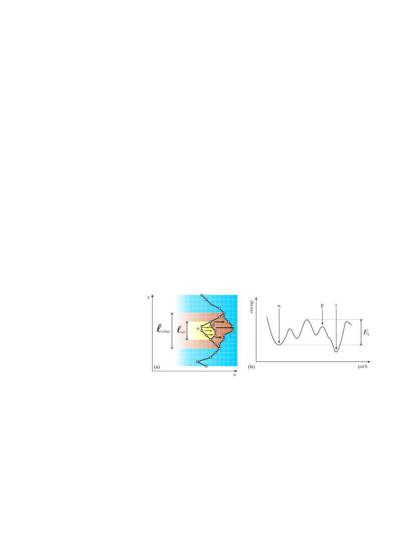
Figure 2: Low temperature dynamics of the driven elastic string below the depinning threshold. The optimal path to escape from a given metastable configuration $\alpha$ pass through a saddle configuration $\beta$, from which the system is able to relax deterministically to the next metastable configuration $\gamma$ with $E_{\gamma}<E_{\alpha}$.

For non-zero drive but still below the depinning threshold ($0<f<f_{c}$), a finite temperature must be imposed in order to forget the initial condition and reach a unique stationary state. In references [31, 32] the regime relevant for creep motion was studied; this is, the steady state regime of an interface in the limit of vanishing temperature. A direct numerical study of the motion of such regime is very difficult. The motion takes place by thermal activation over barriers leading to extremely long activation times making numerical techniques such as the Langevin dynamics inefficient. Fortunately, different numerical method [31, 32] allows to follow the motion of an interface at finite temperature, avoiding the above-mentioned difficulty. This method directly implements the polymer dynamics as a unique forward-moving sequence of metastable states of decreasing energy. It can be proved that such a sequence corresponds to the exact dynamics for a finite interface in a given disorder realization in the $T\to 0$ limit.

The elementary step of such a dynamics is sketched in Fig. 2. It consists in finding the optimal path from one metastable configuration $\alpha$ with energy $E_{\alpha}$ to the next metastable configuration $\gamma$, with a lower energy. This path pass through a saddle configuration $\beta$ with an energy $E_{\beta}>E_{\alpha}$. Once in $\beta$ the polymer relaxes deterministically to $\gamma$. The configurations $\alpha$ and $\gamma$ differ from each other by a portion of size ${{\ell}_{\tt relax}}$, while $\alpha$ and $\beta$ differ by ${{\ell}_{\tt opt}}$. The maximun energy $E_{\tt max}$ reached by the polymer through the path defines a drive dependent barrier $E_{b}(f)=E_{\tt max}-E_{\alpha}$, therefore the time associated to this elementary step is given by $\sim e^{E_{b}(f)/T}$.

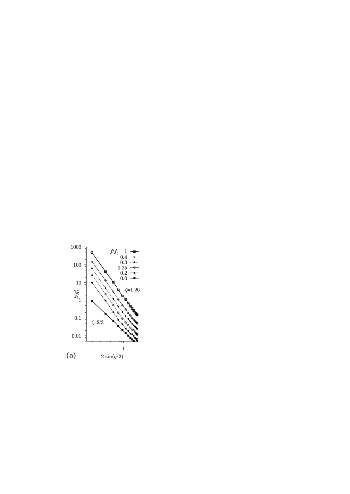
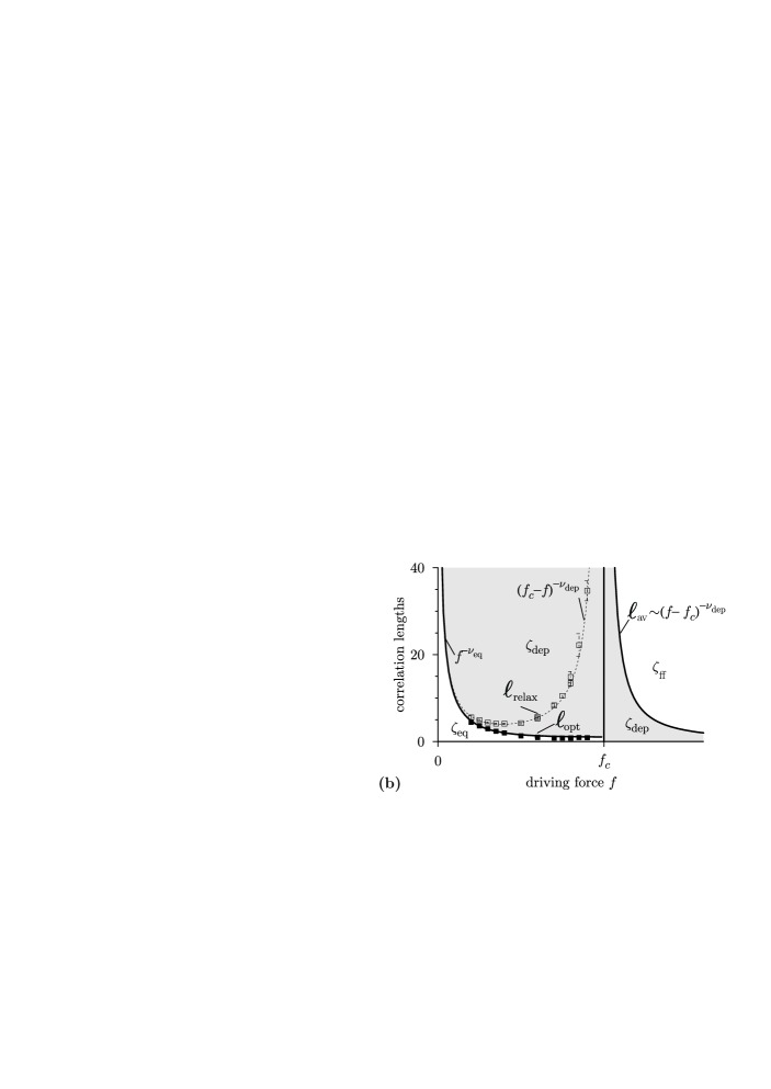
Figure 3: (a) Steady state structure factor $S(q)$ of the line in the $T\rightarrow 0$ limit for different forces (curves are shifted for clarity). (b) The steady state properties of the elastic string at $T\rightarrow 0$ are determined by ${{\ell}_{\tt opt}}$ (filled symbols) and by ${{\ell}_{\tt av}}$. These lengths separate regions characterized by the equilibrium exponent, the depinning exponent (gray region), and the fast flow one. The divergent length ${{\ell}_{\tt relax}}$ (open symbols) is associated only with transient dynamics. Lines are guides to the eye. Figures are adapted with permission from [31].

Numerical results are summarized in Fig. 3: (i) The structure factor behavior below $f_{c}$ supports the picture proposed in Fig. 1. In particular this behavior is consistent with FRG calculations [16] that predict in the creep regime the existence of a characteristic scale (namely ${{\ell}_{\tt opt}}$) below which the system is at equilibrium and above which the system is characterized by deterministic forward motion. Moreover, in qualitative agreement with these predictions it is observed that both ${{\ell}_{\tt opt}}$ and $E_{b}(f)$ increase as $f$ decreases. Unfortunately this algorithm has not allowed to explore the region of vanishing $f$ where ${{\ell}_{\tt opt}}$ is expected to diverge as $\sim f^{-1/(2-{\zeta_{\tt eq}})}$ and the “optimal” barrier as $E_{b}(f)\sim f^{-\mu}$. In turn, it can be seen that the size ${{\ell}_{\tt rel}}$ diverges as $\sim(f_{c}-f)^{-{\nu_{\tt dep}}}$ and this is interpreted as the linear size of the deterministic depinning-like avalanche triggered by thermal nucleation. It is worth remarking that although ${{\ell}_{\tt relax}}$ diverges as $f\to f_{c}$ from below, it does not affect the steady-state spatial correlations, unlike ${{\ell}_{\tt av}}$ and ${{\ell}_{\tt opt}}$.

In order to study the effects of larger temperatures one can use Langevin dynamics [39]. These simulations show that ${{\ell}_{\tt av}}$ has a finite value for $T>0$ and $0<f<f_{c}$ and it actually diverges as $f\to 0$ (as sketched in Fig. 1), but the lack of precison does not allow to test the universal behavior ${{\ell}_{\tt av}}\sim T^{-\sigma}f^{-\lambda}$ predicted by FRG calculations [16]. Note that ${{\ell}_{\tt av}}$ diverges as the velocity goes to zero, while ${{\ell}_{\tt relax}}$ remains finite in the same limit. In other words, while in the $T\to 0$ limit the string is blocked in the first metastable state with lower energy producing an avalanche of typical size ${{\ell}_{\tt relax}}$, at finite temperature a larger avalanche of size ${{\ell}_{\tt av}}$ takes place. In the creep regime these depinning-like processes are fast in comparison with the waiting times for the thermally activated jumps (${{\ell}_{\tt opt}}$).

Finally, the finite temperature long time relaxation of a flat line in absence of drive can be described as a creep process over barriers that increase in time, such that the growing correlation length (separating the equilibrated length-scales with the ones retaining memory of the initial condition) is [47] $\ell(t)\sim[T\log(t)]^{1/\theta}$.

4.3 Depinning regime at $T=0$

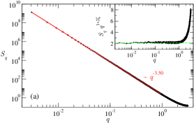
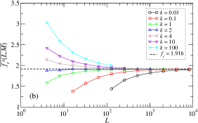
Figure 4: Results for the critical state in finite samples obtained with the exact algorithm of Sec. 4.3.1. (a) Critical configuration structure factor (see definition in Eq. (6)). The fitted roughness exponent yields ${\zeta_{\tt dep}}=1.250\pm 0.005$. (b) The finite-size critical force $f_{c}$ as a function of the longitudinal size $L$ for periodic samples of size $L\times M$ with $M=kL^{\zeta_{\tt dep}}$. As $L$ grows the asymptotic value of the critical threshold becomes independent on the aspect ratio $k$. The dashed line corresponds to the thermodynamic limit $f_{c}=1.916\pm 0.001$. Figures are reproduced with permission from [41].

4.3.1 Critical force and critical configuration

At $T=0$, the transition between a pinned phase and a moving phase is displayed in any finite sample with a given disorder realization. This is assured by a set of properties pointed out by Middleton [48]. The first one is the so-called “no-passing rule”: if two strings $u(x,t)$ and $\tilde{u}(x,t)$ do not cross at a given time, they will not cross at any later times. Another important property of Middleton’s theorem states that if, at an initial time, the velocities are non-negative for all points $x$, they will remain non-negative for all later times. It follows from these properties that, once we have found a forward moving string, we can be sure that snapshots of the string at later times will be ahead (in the $u$ direction). As a consequence of these two properties, we can define (for a given finite sample) the critical force $f_{c}^{\tt{sample}}$ as the maximal force for which a metastable configuration still exists; i.e., a configuration for which al points $x$ verify $\partial_{t}u(x,t)=0$. Analogously to the ground state polymer for the statics (Sec. 4.1), this last unique metastable configuration displays self-affine properties with a well defined roughness exponent $\zeta_{dep}$ (see Fig. 4a). For a finite sample, $f_{c}^{\tt{sample}}$ is a stochastic variable which depends on the disorder realization. As the size $L$ of the sample grows, the asymptotic critical threshold $f_{c}$ is approached (see Fig. 4b), and the fluctuations of $f_{c}^{\tt{sample}}$ are suppressed as [49]

$$\overline{\left[f_{c}^{\tt{sample}}\right]^{2}}-\left[\overline{f_{c}^{\tt{sample}}}\right]^{2}\sim L^{-2/{\nu_{\tt dep}}};$$ (9)

where ${\nu_{\tt dep}}$ is the characteristic correlation length exponent. Both the exponents $\zeta_{dep}$ and $\nu_{dep}$ can be carefully determined using numerical algorithms that avoid the direct numerical integration of Eq. (1). The key idea behind these methods is to check for the existence of metastable states for the string in the particular sampled disorder for a given value of the external force $f$. This check can be performed in a computing time that grows only linearly with the system size using properties discussed by Middleton [40, 50].

4.3.2 Critical and dynamical exponents: the non-steady relaxation

The accurate determination of critical exponents is a difficult task, specially for critical phenomena in disordered systems. The so-called Short-Time Dynamics method (STD) allows to obtain critical exponents values without the need of system equilibration. It relies on the validity of an homogeneous relation for the order parameter when the system performs a non-steady relaxation at the critical point. This scaling relation, in contrast with traditional equilibrium finite-size scaling methods, can be used to avoid finite-size effects but includes dependences with time and initial conditions [51, 52, 53].

To apply the STD to the depinning transition we rely on the analogy with standard phase transitions [36]. By considering the velocity $v$ as an order parameter, and the dimensionless force $(f-f_{c})/f_{c}$ as the reduced driving field, we expect the following homogeneity relation to be valid for the long-time relaxation of an initially flat string (infinite velocity initial condition) [54, 55, 41]:

$$v(h,L,t)=t^{-\beta/\nu z}\tilde{v}_{\pm}(t^{1/z\nu}h,t^{-1/z}L);$$ (10)

where $h=|f-f_{c}|/f_{c}$ and the function $\tilde{v}_{\pm}$ has two branches depending on the sign of $f-f_{c}$. Close to depinning, the relaxational dynamics described by Eq. (10) is valid in a short-time regime, after which the velocity reaches a steady-state value if $f>f_{c}$, while for $f<f_{c}$ the string is blocked in a metastable state (with memory of the initial condition) and $v\to 0$. Exactly at the critical point ($h=0$) and in the limit $L\to\infty$ we expect a power-law behavior for the velocity, $v\sim t^{-\beta/\nu z}$. Alternatively, we can write $v\sim\ell(t)^{-\beta/\nu}$, where $\ell(t)\sim t^{1/z}$ is the dynamical length, describing the growth of roughness as $w(t)\sim\ell(t)^{\zeta}\sim t^{\zeta/z}$. By fitting $v(t)$ and $w(t)$ we thus in principle get $\beta/\nu z$ and ${\zeta/z}$ independently. Since $\zeta$ (and therefore $\nu$) can be obtained independently using the method described in Sec. 4.3.1, with the STD method it is possible to extract in addition the critical exponent $\beta$ and the dynamical exponent $z$.

In Ref. [41] large scale Langevin dynamics simulations have been implemented to obtain $v(t)$ and $w(t)$ over a large period of time for large system sizes, such that $L\gg\ell(t)$. This has allowed to detect robust (under different shape and nature of the disorder correlator) scaling corrections to the asymptotic power-law forms, and thus to avoid fitting effective power-law decays, yielding significantly biased incorrect exponents. A practical criterion to estimate the crossover between the “mesoscopic” time regime with corrections and the truly universal “macroscopic” time regime was found by observing that the hyperscaling relation $\beta=\nu(z-\zeta)$ is violated in the former regime. This can be easily seen by analyzing the quantity $\gamma(t)=\frac{w(t)}{tv(t)}$: if the measured $\gamma(t)$ depends on time, it means that the system has not reached the critical scaling regime yet.

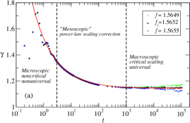
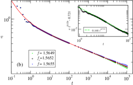
Figure 5: Evolution of $\gamma(t)$ (a) and $v(t)$ (b) for $f\approx f_{c}$, with $f_{c}$ the thermodynamic critical force. Two other forces, just above ($f_{c}^{+}$) and just below ($f_{c}^{-}$) $f_{c}$ are also shown. Continuous lines are fits for $\gamma(t)$ and $v(t)$ including power-law corrections to the asymptotic scaling yielding the true critical exponents. In (a) vertical dashed lines separate qualitatively different time regimes. The inset in (b) shows that corrections to scaling are power-law like. Figures are adapted with permission from [41].

In Fig. 5(a) we show the behavior of $\gamma(t)$. After a microscopic regime, $\gamma(t)$ slowly decreases implying an “effective” unbalanced relation $\left[\nu(z-\zeta)-\beta\right]_{\mathrm{eff}}<0$. In this mesoscopic regime the critical dynamics scaling is not valid. After a surprisingly long crossover however, $\gamma(t)$ develops a plateau. This information allows to determine the appropriate time regime of $v(t)$ and $w(t)$ where it is possible to fit $\beta/\nu z$ and $\zeta/z$, respectively. In Fig. 5(b) the behavior of $v(t)$ is shown. Power-law corrections of the form $v(t)=V_{0}\leavevmode\nobreak\ t^{-\beta/\nu z}\left[1+\left({t}/{t_{v}}\right)^{-\alpha_{v}}\right]$ (with $V_{0}$, $t_{v}$, and $\alpha_{v}$ fitting parameters) are find. At large times, when $\gamma(t)$ develops a plateau, an accurate power-law fit can be performed for $v(t)$ at the thermodynamic depinning force $f_{c}=1.5652\pm 0.0003$, yielding $\beta/(\nu z)=0.128\pm 0.003$. The observation of scaling corrections explain the systematically larger effective values for $(\beta/\nu z)$ reported before for smaller systems [41]. An analogous analysis for $w(t)$ shows similar robust power-law scaling corrections, and gives a consistent value for the exponent, $1-\zeta/z=0.128\pm 0.003$. These results, combined with an independently determined value of $\zeta=1.250\pm 0.005$ (see Fig. 4a) and the relation $\nu=1/(2-\zeta)$, allows to get $\beta=0.245\pm 0.006$, $z=1.433\pm 0.007$, $\zeta=1.250\pm 0.005$ and $\nu=1.333\pm 0.007$ [41]. Scaling forms for the joint force-time dependence of the velocity extracted from Eq. (10) are in excellent agreement with these exponents [41].

4.4 Depinning regime at $T>0$: the critical thermal rounding

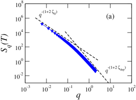
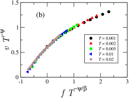
Figure 6: (a) Structure factor $S_{q}$ at a finite temperature $T=0.02$ showing two regimes with different roughness exponents, ${\zeta_{\tt ff}}$ and ${\zeta_{\tt dep}}$, above and below the crossover length scale ${{\ell}_{\tt av}}$, respectively. (b) Velocity-force scaling function in the thermal rounding region. The disorder intensity is kept fixed and the velocity for different temperatures collapses in a single function. Figures are adapted with permission from [43].

When the temperature is finite, there is no sharp transition between zero and finite velocity regimes. At forces around the critical value, $f\approx f_{c}$, a finite temperature value smears out the transition, which is no longer abrupt. This thermal rounding of the depinning transition can be characterized, exactly at the critical force $f=f_{c}$, by a power-law vanishing of the velocity with the temperature $v\sim T^{\psi}$, where $\psi$ is the so-called the thermal rounding exponent [38, 42, 43, 56, 57].

At small length scales, $q\gg 1/{{\ell}_{\tt av}}$, the structure factor shows the typical roughness regime associated to depinning, i.e. $S_{q}\sim q^{-(1+2{\zeta_{\tt dep}})}$, while at large length scales, $q\ll 1/{{\ell}_{\tt av}}$, geometrical properties are dictated by effective thermal fluctuations induced by the disorder, i.e. $S_{q}\sim q^{-(1+2{\zeta_{\tt ff}})}$, as shown in Fig. 6(a). In the critical region the depinning correlation length is given by the velocity as ${{\ell}_{\tt av}}\sim v^{-\nu/\beta}$. Thus, the depinning correlation length depends on the temperature only through the velocity and in the thermal rounding regime [42] ${{\ell}_{\tt av}}\sim T^{-\psi\nu/\beta}$. With this information one can write for the structure factor

$$S_{q}=T^{-\psi{\nu_{\tt dep}}(1+2{\zeta_{\tt dep}})/\beta}s\left(qT^{-\psi{\nu_{\tt dep}}/\beta}\right),$$ (11)

where the scaling function $s(y)\sim y^{-(1+2{\zeta_{\tt ff}})}$ for $y\ll 1$ and $s(y)\sim y^{-(1+2{\zeta_{\tt dep}})}$ for $y\gg 1$. In Ref. [42] it was shown that the structure factor scales with the previous form.

All the information about the thermal rounding regime can be gathered in the expected universal behavior of $v(h,T)$. It is possible to show that assuming the homogeneous relation between the velocity and both temperature and force, as it is usual for phase transitions, a universal function follows. If there were not strong finite size effects, in the vicinity of the critical region the velocity should scale as

$$vT^{-\psi}\sim h_{\pm}\left(fT^{-\psi/\beta}\right),$$ (12)

with $h_{\pm}(x)$ a universal function which can in principle be different above ($h_{+}$) and below ($h_{-}$) threshold. One expects that $h_{+}\sim y^{\beta}$ for $y\gg 1$. Figure 6(b) shows this scaling relation for fixed disorder intensity and different temperatures as indicated. This universal behavior has been numerically confirmed using Langevin dynamics simulations of the QEW equation [43] and indirectly tested in experiments of domain wall motion in 2D ferromagnets [58].

5 Conclusions and Perspectives

The driven QEW model represents a minimal paradigmatic model for studying the dynamics of driven elastic systems in random media. In this paper we have reviewed a series of numerical methods specially developed for studying different and key properties of this system. The results found in the literature, lead us to the physical picture discussed in Sec. 2 and ilustrated in Fig. 1.

The most challenging aspect of the problem remains the quantitative comparison with experiments. On one hand, it would be important to make quantitative predictions for different elastic universality classes. Although we expect the same basic physics described here to emerge at large enough scales, it is important to accurately obtain the corresponding critical exponents and to understand the additional dynamical crossovers that may arise at intermediate length-scales.

At last, probably the least understood but still experimentally relevant phenomena for the dynamics of interfaces in random media are: the occurrence of “plasticity” (displayed by overhangs and bubbles [59]), the effect of internal degrees of freedom (such as the “spin phase” coupled to the position of magnetic domain walls  [5, 60]), and the effect of “structural relaxation” [15] in host materials. This may encourage the development of new models and novel efficient numerical approaches in the field.

References

- [1] S. Lemerle, J. Ferré, C. Chappert, V. Mathet, T. Giamarchi, P. Le Doussal, Domain wall creep in an ising ultrathin magnetic film, Phys. Rev. Lett. 80 (1998) 849.
- [2] M. Bauer, A. Mougin, J. P. Jamet, V. Repain, J. Ferré, R. L. Stamps, H. Bernas, C. Chappert, Deroughening of domain wall pairs by dipolar repulsion, Phys. Rev. Lett. 94 (2005) 207211.
- [3] M. Yamanouchi, D. Chiba, F. Matsukura, T. Dietl, H. Ohno, Velocity of domain-wall motion induced by electrical current in the ferromagnetic semiconductor (ga,mn)as, Phys. Rev. Lett. 96 (2006) 096601.
- [4] P. J. Metaxas, J. P. Jamet, A. Mougin, M. Cormier, J. Ferré, V. Baltz, B. Rodmacq, B. Dieny, R. L. Stamps, Creep and flow regimes of magnetic domain-wall motion in ultrathin pt/co/pt films with perpendicular anisotropy, Phys. Rev. Lett. 99 (2007) 217208.
- [5] J.-C. Lee, K.-J. Kim, J. Ryu, K.-W. Moon, S.-J. Yun, G.-H. Gim, K.-S. Lee, K.-H. Shin, H.-W. Lee, S.-B. Choe, Universality classes of magnetic domain wall motion, Phys. Rev. Lett. 107 (2011) 067201.
- [6] P. Paruch, T. Giamarchi, J. M. Triscone, Domain wall roughness in epitaxial ferroelectric pbzr0.2ti0.8o3 thin films, Phys. Rev. Lett. 94 (2005) 197601.
- [7] P. Paruch, J. M. Triscone, High-temperature ferroelectric domain stability in epitaxial pbzr0.2ti0.8o3 thin films, Appl. Phys. Lett. 88 (2006) 162907.
- [8] J. Y. Jo, S. M. Yang, T. H. Kim, H. N. Lee, J.-G. Yoon, S. Park, Y. Jo, M. H. Jung, T. W. Noh, Nonlinear dynamics of domain-wall propagation in epitaxial ferroelectric thin films, Phys. Rev. Lett. 102 (2009) 045701.
-
[9]
P. Paruch, A. B. Kolton, X. Hong, C. H. Ahn, T. Giamarchi,
Thermal quench
effects on ferroelectric domain walls, Phys. Rev. B 85 (2012) 214115.
doi:10.1103/PhysRevB.85.214115.
URL http://link.aps.org/doi/10.1103/PhysRevB.85.214115 -
[10]
J. Guyonnet, E. Agoritsas, S. Bustingorry, T. Giamarchi, P. Paruch,
Multiscaling
analysis of ferroelectric domain wall roughness, Phys. Rev. Lett. 109 (2012)
147601.
doi:10.1103/PhysRevLett.109.147601.
URL http://link.aps.org/doi/10.1103/PhysRevLett.109.147601 - [11] S. Moulinet, A. Rosso, W. Krauth, E. Rolley, Width distribution of contact lines on a disordered substrate, Phys. Rev. E 69 (2004) 035103(R).
-
[12]
Le Doussal, P., Wiese, K. J., Moulinet, S., Rolley, E.,
Height fluctuations of a
contact line: A direct measurement of the renormalized disorder correlator,
EPL 87 (5) (2009) 56001.
doi:10.1209/0295-5075/87/56001.
URL http://dx.doi.org/10.1209/0295-5075/87/56001 - [13] E. Bouchaud, J. P. Bouchaud, D. S. Fisher, S. Ramanathan, J. R. Rice, Can crack front waves explain the roughness of cracks?, J. Mech. Phys. Solids 50 (2002) 1703.
- [14] D. Bonamy, S. Santucci, L. Ponson, Crackling dynamics in material failure as the signature of a self-organized dynamic phase transition, Phys. Rev. Lett. 101 (4) (2008) 045501. doi:10.1103/PhysRevLett.101.045501.
- [15] E. A. Jagla, A. B. Kolton, A mechanism for spatial and temporal earthquake clustering, J. Geophys. Res. 115 (2010) B05312.
- [16] P. Chauve, T. Giamarchi, P. Le Doussal, Phys. Rev. B 62 (2000) 6241.
- [17] T. Giamarchi, S. Bhattacharya, in: C. Berthier et al. (Ed.), High Magnetic Fields: Applications in Condensed Matter Physics and Spectroscopy, Springer-Verlag, Berlin, 2002, p. 314, cond-mat/0111052.
- [18] T. Nattermann, S. Brazovskii, Pinning and sliding of driven elastic systems: from domain walls to charge density waves, Adv. Phys. 53 (2004) 177.
- [19] H. Gao, J. R. Rice, J. Appl. Mech. 56 (1989) 828.
-
[20]
A. Tanguy, M. Gounelle, S. Roux,
From individual to
collective pinning: Effect of long-range elastic interactions, Phys. Rev. E
58 (1998) 1577–1590.
doi:10.1103/PhysRevE.58.1577.
URL http://link.aps.org/doi/10.1103/PhysRevE.58.1577 - [21] D. Bonamy, E. Bouchaud, Failure of heterogeneous materials: A dynamic phase transition?, Phys. Rep. 498 (2011) 1.
- [22] M. Alava, P. K. V. V. Nukalaz, S. Zapperi, Statistical models of fracture, Adv. Phys. 55 (2006) 349.
- [23] J. F. Joanny, P.-G. de Gennes, A model for contact angle hysteresis, J. Chem. Phys. 81 (1984) 552.
- [24] P. Le Doussal, K. J. Wiese, S. Moulinet, E. Rolley, Height fluctuations of a contact line: A direct measurement of the renormalized disorder correlator, Europhys. Lett. 87 (5) (2009) 56001.
- [25] A. Rosso, W. Krauth, Phys. Rev. Lett. 87 (2001) 187002.
- [26] L.-H. Tang, M. Kardar, D. Dhar, Driven depinning in anisotropic media, Phys. Rev. Lett. 74 (6) (1995) 920–923. doi:10.1103/PhysRevLett.74.920.
- [27] Image of the magnetic contrast in a Co/Pt/Co film obtained by MOKE. Courtesy J. Ferre.
- [28] E. Agoritsas, V. Lecomte, T. Giamarchi, Temperature-induced crossovers in the static roughness of a one-dimensional interfase, Phys. Rev. B 82 (2010) 184207.
- [29] E. Agoritsas, V. Lecomte, T. Giamarchi, Disordered elastic systems and one-dimensional interfaces, Physica B 407 (2012) 1725.
-
[30]
B. Drossel, M. Kardar,
Scaling of energy
barriers for flux lines and other random systems, Phys. Rev. E 52 (1995)
4841–4852.
doi:10.1103/PhysRevE.52.4841.
URL http://link.aps.org/doi/10.1103/PhysRevE.52.4841 - [31] A. B. Kolton, A. Rosso, T. Giamarchi, W. Krauth, Dynamics below the depinning threshold in disordered elastic systems, Phys. Rev. Lett. 97 (2006) 057001.
- [32] A. B. Kolton, A. Rosso, T. Giamarchi, W. Krauth, Creep dynamics of elastic manifolds via exact transition pathways, Phys. Rev. B 79 (2009) 184207.
- [33] D. S. Fisher, D. A. Huse, Directed paths in a random potential, Phys. Rev. B 43 (1991) 10728.
- [34] S. F. Edwards, D. R. Wilkinson, Proc. R. Soc. A 381 (1982) 17.
- [35] J. Krug, Origins of scale invariance in growth processes, Adv. Phys. 46 (1997) 139.
- [36] D. S. Fisher, Sliding charge-density waves as a dynamic critical phenomenon, Phys. Rev. B 31 (1985) 1396.
-
[37]
D. A. Huse, C. L. Henley,
Pinning and
roughening of domain walls in ising systems due to random impurities, Phys.
Rev. Lett. 54 (1985) 2708–2711.
doi:10.1103/PhysRevLett.54.2708.
URL http://link.aps.org/doi/10.1103/PhysRevLett.54.2708 - [38] L. W. Chen, M. C. Marchetti, Interface motion in random media at finite temperature, Phys. Rev. B 51 (1995) 6296.
- [39] A. B. Kolton, A. Rosso, T. Giamarchi, Creep motion of an elastic string in a random potential, Phys. Rev. Lett. 94 (2005) 047002.
- [40] A. Rosso, W. Krauth, Roughness at the depinning threshold for a long-range elastic string, Phys. Rev. E 65 (2) (2002) 025101. doi:10.1103/PhysRevE.65.025101.
-
[41]
E. E. Ferrero, S. Bustingorry, A. B. Kolton,
Nonsteady
relaxation and critical exponents at the depinning transition, Phys. Rev. E
87 (2013) 032122.
doi:10.1103/PhysRevE.87.032122.
URL http://link.aps.org/doi/10.1103/PhysRevE.87.032122 - [42] S. Bustingorry, A. B. Kolton, T. Giamarchi, Thermal rounding of the depinning transition, Europhys. Lett. 81 (2008) 26005.
- [43] S. Bustingorry, A. B. Kolton, T. Giamarchi, Thermal rounding exponent of the depinning transition of a string in a random medium, Phys. Rev. E 85 (2012) 021144.
- [44] S. Bustingorry, P. Le Doussal, A. Rosso, Universal high-temperature regime of pinned elastic objects, Phys. Rev. B 82 (2010) 140201.
- [45] M. Prähofer, H. Spohn, Scale invariance of the png droplet and the airy process, J. Stat. Phys. 108 (2002) 1071.
- [46] E. Agoritsas, S. Bustingorry, V. Lecomte, G. Schehr, T. Giamarchi, Finite-temperature and finite-time scaling of the directed polymer free energy with respect to its geometrical fluctuations, pre 86 (2012) 031144.
- [47] A. B. Kolton, A. Rosso, T. Giamarchi, Phys. Rev. Lett. 95 (2005) 180604.
- [48] A. A. Middleton, Phys. Rev. Lett. 68 (1992) 670.
- [49] C. J. Bolech, A. Rosso, Phys. Rev. Lett. 93 (2004) 125701.
- [50] A. Rosso, P. Le Doussal, K. J. Wiese, Numerical calculation of the functional renormalization group fixed-point functions at the depinning transition, Phys. Rev. B 75 (2007) 220201(R).
- [51] H. Janssen, B. Schaub, B. Schmittmann, Z. Phys. B: Condens. Matter 73 (1989) 539.
- [52] B. Zheng, in Computer simulation studies in condensed-matter physics, Springer, New York, 2006.
-
[53]
E. V. Albano, M. A. Bab, G. Baglietto, R. A. Borzi, T. S. Grigera, E. S.
Loscar, D. E. Rodriguez, M. L. Rubio Puzzo, G. P. Saracco,
Study of phase
transitions from short-time non-equilibrium behaviour, Reports on Progress
in Physics 74 (2) (2011) 026501.
URL http://stacks.iop.org/0034-4885/74/i=2/a=026501 - [54] A. B. Kolton, A. Rosso, E. V. Albano, T. Giamarchi, Short-time relaxation of a driven elastic string in a random medium, Phys. Rev. B 74 (2006) 140201.
- [55] A. B. Kolton, G. Schehr, P. L. Doussal, Universal nonstationary dynamics at the depinning transition, Phys. Rev. Lett. 103 (2009) 160602.
- [56] A. A. Middleton, Thermal rounding of the charge-density-wave depinning transition, Phys. Rev. B 45 (1992) 9465.
- [57] U. Nowak, K. D. Usadel, Influence of temperature on the depinning transition of driven interfaces, Europhys. Lett. 44 (1998) 634.
- [58] S. Bustingorry, A. B. Kolton, T. Giamarchi, Thermal rounding of the depinning transition in ultrathin pt/co/pt films, Phys. Rev. B 85 (2012) 214416.
- [59] V. Repain, M. Bauer, J.-P. Jamet, J. Ferré, A. Mougin, C. Chappert, H. Bernas, Creep motion of a magnetic wall: Avalanche size divergence, epl 68 (2004) 460.
-
[60]
V. Lecomte, S. E. Barnes, J.-P. Eckmann, T. Giamarchi,
Depinning of domain
walls with an internal degree of freedom, Phys. Rev. B 80 (2009) 054413.
doi:10.1103/PhysRevB.80.054413.
URL http://link.aps.org/doi/10.1103/PhysRevB.80.054413