Directional genetic differentiation and relative migration

Abstract

Understanding the population structure and patterns of gene flow within species is of fundamental importance to the study of evolution. In the fields of population and evolutionary genetics, measures of genetic differentiation are commonly used to gather this information. One potential caveat is that these measures assume gene flow to be symmetric. However, asymmetric gene flow is common in nature, especially in systems driven by physical processes such as wind or water currents. Since information about levels of asymmetric gene flow among populations is essential for the correct interpretation of the distribution of contemporary genetic diversity within species, this should not be overlooked. To obtain information on asymmetric migration patterns from genetic data, complex models based on maximum likelihood or Bayesian approaches generally need to be employed, often at great computational cost. Here, a new simpler and more efficient approach for understanding gene flow patterns is presented. This approach allows the estimation of directional components of genetic divergence between pairs of populations at low computational effort, using any of the classical or modern measures of genetic differentiation. These directional measures of genetic differentiation can further be used to calculate directional relative migration and to detect asymmetries in gene flow patterns. This can be done in a user-friendly web application called divMigrate-online introduced in this paper. Using simulated data sets with known gene flow regimes, we demonstrate that the method is capable of resolving complex migration patterns under a range of study designs.

Keywords: Directional gene flow, Asymmetric migration, Dispersal, Allele frequency data. Running title: Directional relative migration

1 Introduction

Measures of population genetic differentiation are widely used in studies focusing on conservation, management and evolution. Generally, information about the pattern of population structure and the level of differentiation are derived from allele frequency data. The most commonly used measures, utilizing this information, being Wright’s fixation index $F_{st}$ (Wright, , 1943), Nei’s $G_{st}$ (Nei, , 1973), and the more recently introduced $G^{\prime}_{st}$ (Hedrick and Goodnight, , 2005) and $D$(Jost, , 2008), which are independent of gene diversity.

A particularly useful feature of these parameters is that, assuming an island model of population structure, they can be used to estimate migration among populations (Wright, , 1931, 1949; Jost, , 2008). These measures, however, assumes migration to be symmetric (i.e. of equal rate in all directions). For simplification, the term migration is here and for the rest of this paper used interchangeably with the term gene flow.

Structured populations characterized by asymmetric migration is, on the other hand, common in nature. Especially in systems driven by physical transport processes, such as wind or water currents (Pringle et al., , 2011), or those with strong habitat quality gradients, which can lead to competition driven directional dispersal (Paz-Vinas et al., , 2013). In marine environments, ocean currents are known to affect both the dispersal of planktonic and benthic species, the latter often being characterized with a planktonic phase during early stages of development (Siegel et al., , 2003; Cowen and Sponaugle, , 2009). Other examples, where the direction of gene flow can be affected by physical processes, include organism living in river systems (e.g. impassable waterfalls prevent upstream dispersal), as well as wind pollinated plants, mosses and lichen (Muñoz et al., , 2004; Hänfling and Weetman, , 2006; Friedman and Barrett, , 2009).

Both physical processes and density dependent competition can lead to source-sink dynamics among populations (i.e. metapopulation structure). Where this occurs, parameters such as genetic differentiation can be significantly skewed (Dias, , 1996). This, in turn, can lead to incorrect conservation and/or management decisions. For instance, while sink populations of poor quality (i.e. low/no intra-population recruitment) contribute little to the long-term evolutionary potential of the species (Whitlock and McCauley, , 1999) they can display greater genetic differentiation relative to source populations (Whitlock and McCauley, , 1999). As a consequence, they can be incorrectly regarded as a ’unique’ component of the species’ overall diversity, which may misdirect conservation efforts.

In asymmetric systems, it becomes important to estimate directional migration to fully understand the processes leading to genetic structuring of populations, as well as to allow for effective conservation and management decisions to be derived from such information (e.g. Pringle et al., , 2011). For example, when aiming to conserve endangered species, implementing management strategies for source populations is known to be more effective than for sink populations (Dias, , 1996). In addition to the difficulties associated with understanding genetic structure, the absence of information about the symmetry of gene flow can also make the inference of past demographic changes within populations more difficult. For instance, Paz-Vinas et al., (2013) recently demonstrated, using both simulated and empirical data, that the probability of incorrectly inferring past population expansions increased dramatically when populations were characterized by asymmetric patterns of gene flow. Thus, the ability to detect asymmetric migration, when it is present, is essential for the understanding of evolutionary processes that have led to contemporary diversity patterns.

Currently, to obtain information about patterns of migration from genetic data in asymmetric systems, complex mathematical models using maximum likelihood or Bayesian approaches are typically required (e.g. Wilson and Rannala, , 2003; Beerli, , 2009). In these models, a large number of parameters are estimated simultaneously involving complex optimization algorithms, resulting in intensive computational requirements. As a consequence, these models are often used as black boxes implying that users, due to the complexity of these analytical approaches, typically only have a limited understanding of the underlying models and their assumptions. Thus, most users are not in a position to adequately assess when their application is inappropriate.

In contrast, the present study introduces a new, relatively simple and tangible method for the detection of asymmetric migration from allele frequency data. This approach provides robust information on the direction of migration and is intended to fill the gap between existing complex methods for measuring asymmetric migration and symmetric measures of genetic differentiation. The method is based on defining a hypothetical pool of migrants for a given pair of populations and estimating an appropriate measure of genetic differentiation between each of the two populations and the hypothetical pool. The directional genetic differentiation can then be used to estimate the relative levels of migration between the two populations. The larger of the two relative migration values indicates the population that is likely to behave as a source population (i.e. the hypothetical pool of migrants is genetically more similar to this population), while the smaller of the two estimates indicates the population most likely to behave as a sink. By testing whether these two genetic distances are significantly different from one another it is also possible to determine whether migration occurs at a significantly higher rate in one direction over the other. The concept of a hypothetical pool of migrants makes it possible to gain new information about direction of gene flow using regular symmetric measures of genetic differentiation.

This new approach opens up a new dimension of applications where directional measures of genetic differentiation can be used both to explore and detect asymmetric migration patterns. It is argued that this tool will be of major utility in molecular ecological studies where information about the presence/absence of genetic connectivity and its dynamics among populations is of interest. Consider, for example, the benefit of being able to explicitly identify source and sink populations in metapopulations; having the ability to test whether physical barriers precluded gene flow in a particular direction; or the ability to understand the influence of ecosystem processes on gene flow (e.g. is the direction of migration among populations correlated with an ocean current). Accordingly, we present this method as a new tool to researchers interested in a better understanding of the demographic and evolutionary dynamics of populations and species and more specifically on the use of this information for conservation and management.

2 Theory

2.1 Measures of genetic differentiation

For measures of genetic differentiation a value of zero indicate that the allele frequencies among populations are equal, while values larger then zero represent increasing differences (Meirmans and Hedrick, , 2011). Generally, these genetic differentiation measures are based on two parameters, which describe the distribution of genetic diversity among populations, namely, the mean heterozygosity in the total population ($H_{t}$) and the mean heterozygosity within the individual populations ($H_{s}$) (Meirmans and Hedrick, , 2011). While an extensive formal set of notations exists for these two parameters, as well as for $G_{st}$ and $D$, in here we introduce vector notations which make it possible to carry out calculations for a number of populations simultaneously.

Let the total number of different alleles present in $P$ populations be $N$. For now, equal population sizes are assumed. The allele frequencies in the individual populations can then be arranged in the $N\times P$-matrix $A$.

$$A=\left(\begin{array}[]{llll}a_{11}&\cdots&a_{1P}\\ \vdots&\cdots&\vdots\\ a_{N1}&\cdots&a_{NP}\end{array}\right)=\left(\boldsymbol{a_{1}},\cdots,\boldsymbol{a_{P}}\right)\quad,$$ (1)

where the matrix element $a_{ij}$ represents the frequency of allele $i$ in population $j$ with $\sum_{i}a_{ij}=1$ for any population $j$. The column vectors $\boldsymbol{a_{j}}\in[0,1]^{N}$ constitute the allele frequencies in the individual populations, please note that bold letters indicate vectors. For each population, the degree of heterozygosity ($H$) can be estimated from the vector of allele frequencies $\boldsymbol{a}\in[0,1]^{N}$ as:

$${H}(\boldsymbol{a})=1-\boldsymbol{a}^{T}\boldsymbol{a}=1-|\boldsymbol{a}|^{2}\quad.$$ (2)

For a pairwise comparison involving two populations with allele frequencies $\boldsymbol{a}\in[0,1]^{N}$ and $\boldsymbol{b}\in[0,1]^{N}$, within-population heterozygosity ($H_{s}$) and total-population heterozygosity ($H_{t}$) can be estimated from equation (2) as:

$${H_{t}}(\boldsymbol{a},\boldsymbol{b}) = 1-\frac{1}{4}\left|\boldsymbol{a}+\boldsymbol{b}\right|^{2}\quad,$$ (3a)

$${H_{s}}(\boldsymbol{a},\boldsymbol{b}) = 1-\frac{1}{2}\left(|\boldsymbol{a}|^{2}+|\boldsymbol{b}|^{2}\right)\quad.$$ (3b)

From these expressions measures for genetic differentiation between populations with allele frequencies $\boldsymbol{a}$ and $\boldsymbol{b}$ can be defined using vector algebra:

$${D_{st}}(\boldsymbol{a},\boldsymbol{b}) = {H_{t}}(\boldsymbol{a},\boldsymbol{b})-{H_{s}}(\boldsymbol{a},\boldsymbol{b})=\frac{1}{4}|\boldsymbol{a}-\boldsymbol{b}|^{2}\quad,$$ (4a)

$${G_{st}}(\boldsymbol{a},\boldsymbol{b}) = \frac{{D_{st}}(\boldsymbol{a},\boldsymbol{b})}{{H_{t}}(\boldsymbol{a},\boldsymbol{b})}=\frac{|\boldsymbol{a}-\boldsymbol{b}|^{2}}{4-|\boldsymbol{a}+\boldsymbol{b}|^{2}}\quad,$$ (4b)

$${D}(\boldsymbol{a},\boldsymbol{b}) = \frac{2{D_{st}}(\boldsymbol{a},\boldsymbol{b})}{1-{H_{s}}(\boldsymbol{a},\boldsymbol{b})}=\frac{|\boldsymbol{a}-\boldsymbol{b}|^{2}}{|\boldsymbol{a}|^{2}+|\boldsymbol{b}|^{2}}\quad.$$ (4c)

Expressions (4) are equivalent to the (biased) estimators used for calculation of genetic differences as compiled e.g. in (Jost, , 2008). Multi-locus $D$ is calculated as by (Crawford, , 2010) and multi-locus $G_{ST}$ is calculated as proposed in (Nei, , 1973).

2.2 A new concept for estimating directional measures of genetic differentiation

To introduce the new analytic approach, the following hypothetical scenario is considered. Assuming two populations A and B with strong directional gene flow in the direction A $\rightarrow$ B, but no gene flow in the opposite direction, (e.g. as observed when waterfalls prevent or restrict movement in a single direction for species in river systems). In addition, population B may exchange genes with other populations that are genetically distinct from A and which contain alleles not present in A. How would such a situation be reflected in the allelic frequencies? Generally, it can be expected that most alleles present in A are also present in population B, whereas alleles present in B may or may not be present in A due to the absence of gene flow from B to A.

In the case of neutral loci the relative allele frequencies of A are expected to be reflected in the migration and therefore the proportions of the allele frequencies is assumed to be equal in population B. An idealized example of an allelic matrix (A) is listed in Table 1. In this example alleles 1 and 2, present in population A are represented at reduced frequencies but equal proportions in population B, whereas allele 3 is only present in population B. From the distribution of allele frequencies it becomes evident, that there is no gene flow from B to A, but at least some degree of gene flow from A to B cannot be ruled out.

This concept can be formalized as follows; for each mutual pair of populations to be investigated (populations A and B in this example), a hypothetical pool of migrants with an allelic composition inferred from the two populations surveyed is introduced. That is, the hypothetical population has an allelic distribution $\boldsymbol{f}(\boldsymbol{a},\boldsymbol{b})$. The allelic frequencies represented in the pool are calculated as the (normalized) geometrical means of the allelic frequencies in the corresponding two populations of interest: $f_{i}(\boldsymbol{a},\boldsymbol{b})=\gamma\sqrt{a_{i}b_{i}}$ with $\gamma=\left(\sum_{i}\sqrt{a_{i}b_{i}}\right)^{-1}$ if $\sum_{i}\sqrt{a_{i}b_{i}}>0$ and $\gamma=0$ otherwise.

Let us present a general motivation of this definition of the hypothetical pool of migrants. From the hypothetical scenario a number of requirements for the hypothetical pool $\boldsymbol{f}(\boldsymbol{a},\boldsymbol{b})$ are defined:

1. $\boldsymbol{f}(\boldsymbol{a},\boldsymbol{b})$ should be symmetric in its arguments, since the order of populations is arbitrary.

2. Alleles not represented in one of the populations can be assumed not to be relevant for gene flow. As a consequence $\boldsymbol{f}$ should be non-zero only for alleles present at non-zero frequencies in both populations.

A general form for $\boldsymbol{f}(\boldsymbol{a},\boldsymbol{b})$ consistent with these two conditions would be

$$f_{i}(\boldsymbol{a},\boldsymbol{b})=\gamma\sum_{k=1}^{K}\gamma_{k}\left(a_{i}^{\alpha_{k}}b_{i}^{\beta_{k}}+a_{i}^{\beta_{k}}b_{i}^{\alpha_{k}}\right)\quad\forall i$$ (5)

with arbitrary exponents $\alpha_{k},\beta_{k}>0$ for all $k$, an arbitrary $K$ defining the number of summands involved and arbitrary weighting and normalization constants $\gamma$ and $\gamma_{k}$. Here arbitrary means, that at this stage any function defined through any arbitrary set of the parameters above would be consistent with considerations 1 and 2. In this vein equation (5) defines a quite general class of functions.

In the optimal example data discussed in connection with the hypothetical scenario (Table 1) $a_{1}/a_{2}=b_{1}/b_{2}$, which mirrors the fact that the proportions of alleles $1$ and $2$ in population 1 is reflected in the gene flow and transferred to population 2. In order to be consistent with the hypothetical scenario, the pool of migrants is required to reproduce this proportion of alleles as well:

1. In case of strong gene flow only occurring in one direction between populations, initially with mutually different alleles, $f_{i}(\boldsymbol{a},\boldsymbol{b})/f_{j}(\boldsymbol{a},\boldsymbol{b})=a_{i}/a_{j}=b_{i}/b_{j}$ is required for all combination of alleles $i$ and $j$ present in both populations.

2. As a vector of allele frequencies $\boldsymbol{f}$ needs to be normalized, i.e. it needs to fulfill $\sum_{i}f_{i}=1$.

From the 3rd requirement on $\boldsymbol{f}$ it can be defined that $\alpha_{k}+\beta_{k}=1$ for any $k$, making an equation of the form

$$f_{i}(\boldsymbol{a},\boldsymbol{b})=\gamma\sum_{k=1}^{K}\gamma_{k}\left(a_{i}^{\alpha_{k}}b_{i}^{1-\alpha_{k}}+a_{i}^{1-\alpha_{k}}b_{i}^{\alpha_{k}}\right)\quad\forall i$$ (6)

with still arbitrary $0<\alpha_{k}<1$ for all $k$, the most general functional approach for the allelic frequencies in the pooled populations. In cases where populations do not share any alleles $\boldsymbol{f}$, will not contain any alleles shared with either of these populations. In such cases, genetic differentiation can be set to $1$ in both directions.

Equation (6) still reflects a vast class of functions, which could meet our conditions. For the time being, and for the rest of this paper, we choose the simplest available function in this class, namely $\alpha_{1}={\gamma}_{1}=1/2$ and $K=1$, resulting in

$$f_{i}(\boldsymbol{a},\boldsymbol{b})=\gamma\sqrt{a_{i}b_{i}}\quad\forall i$$ (7)

with $\gamma=\left(\sum_{i}\sqrt{a_{i}b_{i}}\right)^{-1}$. Hence, the vector of allelic frequencies of the hypothetical population, $\boldsymbol{f}(\boldsymbol{a},\boldsymbol{b})$, is composed of the the normalized geometrical means of the respective components of $\boldsymbol{a}$ and $\boldsymbol{b}$.

As a measure for directional differentiation, both A and B can now be compared to their shared hypothetical pool of migrants $\boldsymbol{f}(\boldsymbol{a},\boldsymbol{b})$. For this purpose, any standard, non-directional measures for genetic differentiation can be applied. Here we choose to use $G_{st}$ and $D$ as introduced in section 2.1.

For the general case of a number of $P$ populations, a $P\times P$-matrix $B$ can be defined, containing the directional measures for genetic differentiation, as

$$B(A,E(\cdot,\cdot))=\left(\begin{array}[]{llll}b_{11}(A,E(\cdot,\cdot))&\cdots&b_{1P}(A,E(\cdot,\cdot))\\ \vdots&\cdots&\vdots\\ b_{P1}(A,E(\cdot,\cdot))&\cdots&b_{PP}(A,E(\cdot,\cdot))\end{array}\right)\quad,$$ (8)

where the individual elements are defined as

$$b_{ij}(A,E(\cdot,\cdot))=E\left(\boldsymbol{a_{i}},\boldsymbol{f}\left(\boldsymbol{a_{i}},\boldsymbol{a_{j}}\right)\right)\quad\forall i,j\quad.$$ (9)

Here, $E(\cdot,\cdot)$ is a place-holder for estimates of genetic differentiation, such as $G_{st}$ and $D$. $A$ is the matrix of allele frequencies containing the population specific allele frequency vectors $\boldsymbol{a}$. The value of a particular matrix element $b_{ij}$ can now be taken as an indicator of the potential for gene flow from population $i$ to population $j$. Low values indicate a high potential for migration, while high values indicate low potential for migration in the direction of interest.

With the idealized example data listed in Table 1, $\boldsymbol{f}(\boldsymbol{a},\boldsymbol{b})=\boldsymbol{a}$, implying that the genetic constitution of A is equal to the hypothetical pool of migrants, whereas the genetic differentiation between the pool and population B is non-zero ($G_{st}(\boldsymbol{b},\boldsymbol{f}(\boldsymbol{a},\boldsymbol{b}))=0.15$ and $D(\boldsymbol{b},\boldsymbol{f}(\boldsymbol{a},\boldsymbol{b}))=0.42$). This result indicates that there is a lower potential for gene flow from B to A than there is from A to B, which is consistent with the initial hypothetical scenario.

It is important to emphasize that, in this paper, we only consider idealized conditions. Thus, the impact of more complex scenarios including, for instance, recent common ancestry, unequal population sizes or populations not being at equilibrium are not considered at this point. The motivation is kept as general and clear as possible to encourage further developments, which allow for adapting the method to more specific and complex conditions. Notwithstanding its simplicity, however, we argue that our model seems to be robust enough to deal with a wide range of conditions.

2.3 Estimations of directional relative migration

Assuming Wright’s infinite island model, $F_{st}$ and by extension $G_{st}$ can directly be related to migration (Wright, , 1931).

$$N_{e}m\approx\frac{((\frac{1}{G_{st}})-1)}{4}$$ (10)

Here we use equation (10) as a step to calculate relative migration, thus either the infinite or finite island model can be used at this point.

Jost outlines in a similar way how $D$ can be used to calculate migration using the finite island model. If we assume, that the mutation rate does not differ between populations $\mu$ can be eliminated from the Equation (22) in Jost (2008) by defining the scaled migration rate $M=m/\mu$. We fixed the number of sampled populations $n$ to two, since we only estimate pairwise comparisons and get

$$M\approx(1-D)/D\quad.$$ (11)

From the effective migration rate in equation (10), and the scaled migration rate in equation (11), relative migration rates between population pairs can be calculated. For now we only focus on relative migration rates to make the method less sensitive to possible inaccuracies in the estimation of effective migration rate and scaled migration rate, due to populations not fitting the assumptions of the island model or not being in drift-mutation equilibrium. Extending this concept to the directional measures of genetic differentiation introduced in the previous section, a similar expression can be used for the estimation of directional relative migration. To this end, a $P\times P$-matrix $C$ of relative migration is defined as

$$C(A)=\left(\begin{array}[]{llll}c_{11}(A)&\cdots&c_{1P}(A)\\ \vdots&\cdots&\vdots\\ c_{P1}(A)&\cdots&c_{PP}(A)\end{array}\right)\quad,$$ (12)

to calculate migration from $G_{st}$ the individual elements are defined as

$$c_{ij}(A)=\frac{((\frac{1}{G_{st}\left(\boldsymbol{a_{i}},\boldsymbol{f}\left(\boldsymbol{a_{i}},\boldsymbol{a_{j}}\right)\right)})-1)}{4}\quad\forall i,j\quad.$$ (13)

to calculate migration from $D$ the individual elements are defined as

$$c_{ij}(A)=\frac{1-D\left(\boldsymbol{a_{i}},\boldsymbol{f}\left(\boldsymbol{a_{i}},\boldsymbol{a_{j}}\right)\right)}{D\left(\boldsymbol{a_{i}},\boldsymbol{f}\left(\boldsymbol{a_{i}},\boldsymbol{a_{j}}\right)\right)}\quad\forall i,j\quad.$$ (14)

The matrix $C$ is then normalized by its biggest value to obtain directional relative migration ranging from zero to one. $A$ is the matrix of allele frequencies containing the population specific allele frequency vectors $\boldsymbol{a}$. The respective matrix elements $c_{ij}(A)$ provide an estimate for the directional relative migration from population $i$ to population $j$. To assess whether gene flow is significantly asymmetric, the directional genetic distances presented in the previous section can be assessed by means of a bootstrap procedure.

3 Simulations

3.1 Methods

To assess the performance of the method described, we evaluate it under variable gene flow patterns and sample designs. This was done by simulating multiple microsatellite data sets from two populations ($N=1000$), under three distinct gene flow patterns (unidirectional gene flow, bidirectional symmetric gene flow and bidirectional asymmetric gene flow). While we acknowledge that these three patterns do not cover all scenarios likely to take place in nature, they are good starting points to begin to assess the potential usefulness of the the new method.

The ability of the proposed new approach to resolve each of these migration patterns was tested for three levels of gene flow as follows: low ($m=0.00025$), medium ($m=0.005$) and high ($m=0.05$), which correspond to population divergence levels of $F_{st}=0.5,0.05,0.005$ using the equation $F_{st}\approx\frac{1}{4N_{e}m+1}$ (Wright, , 1931).

In cases where the pattern was unidirectional, gene flow was simulated in the direction from population two to population one. For the symmetric bidirectional pattern, gene flow was simulated in both directions at an equal rate ($m/2$). For the asymmetric bidirectional pattern gene flow was simulated in both directions, but at $1/4$ from population one to population two and $3/4$ from population two to population one ($m*1/4$ and $m*3/4$).

For each combination of gene flow pattern and gene flow rate, 1000 microsatellite data sets were simulated for each sample size starting with $s=10$ and increasing to $s=100$ in increments of 10 (i.e. $s=10,20,...,100$). This process was repeated for the number of loci, which were also increased from 10 to 100. Three gene flow patterns, under three levels of migration, tested for 10 different sample sizes and 10 different numbers of loci resulted in 180 unique simulation scenarios, for each of which 1000 simulation replicates were generated. When evaluating increasing sample sizes, the number of loci were fixed at 50 and when evaluating the number of loci the sample size was fixed to 50.

For each combination of parameters the number of times out of the 1000 replicates that the method detects higher migration from population two to population one is calculated in percent. For the unidirectional and the asymmetric bidirectional gene flow patterns, the method was expected to detect higher rate in this direction and the result is expected to approach 100%.

In the scenario with symmetric bidirectional gene flow, the method is expected to estimate equally high migration rates in both directions, therefore we do not expect to see a signal. In this scenario, due to random chance, half of the simulations are expected to be higher in one direction and the other half to be higher in the other direction. Thus a value of 50% is the expected outcome.

In all simulations, mutation rate was fixed at $5\times 10^{-4}$, a value which is thought to be common at microsatellite loci in vertebrates (Bhargava and Fuentes, , 2010), and base population size was fixed at $2N=2000$. The performance of the directional migration method was assessed by calculating relative migration rates derived from both $D$ and $G_{st}$. Relative migration rates were calculated using a newly developed R function, divMigrate from the diveRsity package (Keenan et al., , 2013). Simulations were carried out using fastsimcoal2 (Excoffier and Foll, , 2011), and the whole analysis process was scripted in R. Instructions and R scripts to enable readers to reproduce these analyses are available in a dedicated github repository (https://github.com/lisasundqvist/Sundqvist_et_al_2016).

3.2 Results

3.2.1 Unidirectional gene flow

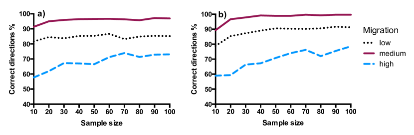
Figure 1: Unidirectional migration: percent correct directions as a function of sample size calculated using $D$ (a) and $G_{st}$ (b). Increasing sample size is evaluated at high ($0.05$), medium ($0.005$) and low ($0.00025$) gene flow. The number of loci are kept fixed at 50.

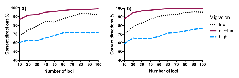
Figure 2: Unidirectional migration: percent correct directions as a function of number of loci calculated using $D$ (a) and $G_{st}$ (b). Increasing number of loci are evaluated at high ($0.05$), medium ($0.005$) and low ($0.00025$) gene flow. The sample size is kept fixed at 50.

The ability of the method to detect the simulated migration from population two to population one was best for the medium migration rate ($m=0.005$). When the sample size reached 20, the correct direction was found in 95% and more of the simulations for both $D$ and $G_{st}$ (figure 1a and 1b). When the number of loci were increased, the result exceeded 95% when the number of loci was 40 for $D$ (figure 2a) and 20 for $G_{st}$ (figure 2b). When the number of loci were 60 or higher the calculations using $G_{st}$ reached 100% correct directions (figure 2b), indicating that the correct direction was detected in all of the 1000 simulations.

The number of correct directions estimated by the method was next highest for low level of migration. For increasing sample size, calculations from $G_{st}$ reached 90% correct directions when the sample size reached 40. When number of loci varied the number of correct directions reached 90% for $D$ when the number of loci was 70 (figure 2a). For $G_{st}$, the result reached 90% when the number of loci was 50 and 95% when the number of loci reached 80 (figure 2b).

When gene flow was high ($m=0.05$), the least number of correct directions was estimated coming close and up to 75% only for the highest sample size and number of loci tested (figure 1 and 2). Increasing sample size had highest effect between 10 and 30 (figure 1). After that, increase in sample size only improve the results when migration was high.

3.2.2 Symmetric bidirectional gene flow

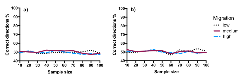
Figure 3: Bidirectional symmetric migration: percent correct directions as a function of sample size calculated using $D$ (a) and $G_{st}$ (b). Increasing sample size is evaluated at high ($0.05$), medium ($0.005$) and low ($0.00025$) gene flow. The number of loci are kept fixed at 50. When migration is symmetric the expected value is 50%.

Figure 3 and 4 clearly demonstrate that the method do not systematically show signs of asymmetry when gene flow is symmetric. All values, even when sample size and number of loci were low, are close to the expected value of 50%. When relative migration was calculated from $G_{st}$ (figure 3b and 4b), the result was slightly more variable than when calculated from $D$ (figure 3a and 4a).

3.2.3 Asymmetric bidirectional gene flow

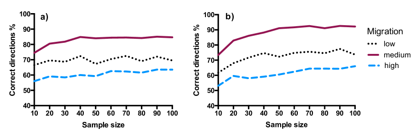
Figure 5: Bidirectional asymmetric migration: percent correct directions as a function of sample size calculated using $D$ (a) and $G_{st}$ (b). Increasing sample size is evaluated at high ($0.05$), medium ($0.005$) and low ($0.00025$) gene flow. The number of loci are kept fixed at 50.

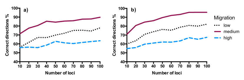
Figure 6: Bidirectional asymmetric migration: percent correct directions as a function of number of loci calculated using $D$ (a) and $G_{st}$ (b). Increasing number of loci are evaluated at high ($0.05$), medium ($0.005$) and low ($0.00025$) gene flow. The sample size is kept fixed at 50.

The usefulness of the method to detect the underlaying migration pattern, which were $1/4$ of the migration rate from population one to population two and $3/4$ from population two to population one ($m*1/4$ and $m*3/4$) is illustrated in figure 5 and 6. The method performs best under medium migration rate ($0.005$). The correct direction was then estimated in over 80% of the times for $D$ and $G_{st}$ (figure 5) when the sample size was 20 and over and reached 90% for $G_{st}$ when the sample size exceeded 50 (figure 5b). When the number of loci increased, the number of correct directions calculated from $D$ reached over 80% when the number of loci was 30 or more (figure 6a). For $G_{st}$ the result reached 80% when the number of loci was 20 and 90% when the number of loci were 50 or more (figure 6b).

When the migration rate was low ($0.00025$), the number of correct directions for estimates calculated from $D$ was below 75% for all sample sizes (figure 5a). For $G_{st}$ (figure 5b), 75% was reached when the sample size reached 40 and stayed around that value as sample size increased further. When the number of loci increased, 75% was reached when the number of loci were 70 for $D$ and 50 for $G_{st}$, (figure 6) and 80% was reached for $G_{st}$ when the number of loci were 70.

When the migration rate was high ($0.05$), the method did not estimate the correct direction at a sufficiently high percentage. However the percentage did increased with sample size and number of loci (figure 6 and 7).

4 Program

To make the new method described in here accessible and easy for people to use, we have developed a web based software application called divMigrate-online. This user friendly interface, provides integrated network visualizations of gene flow patterns among populations, as well as, allowing users to test and visualize significant difference in directional gene flow between pairs of population samples. This section includes a description of the software as well as a demonstration of its use. The flexibility and usefulness of the program are demonstrated by analyzing one simulated data set and one published microsatellite data set of Atlantic salmon (Sandlund et al., 2014b, ).

4.1 About the program

divMigrate-online is designed within the shiny (RStudio & Inc.$2014$) framework for the R programming language (Team $2014$). divMigrate-online is written in the R and C++ programming languages, integrated using the R package Rcpp (Eddelbuettel et al., , 2011) and is hosted at (https://popgen.shinyapps.io/divMigrate-online/).

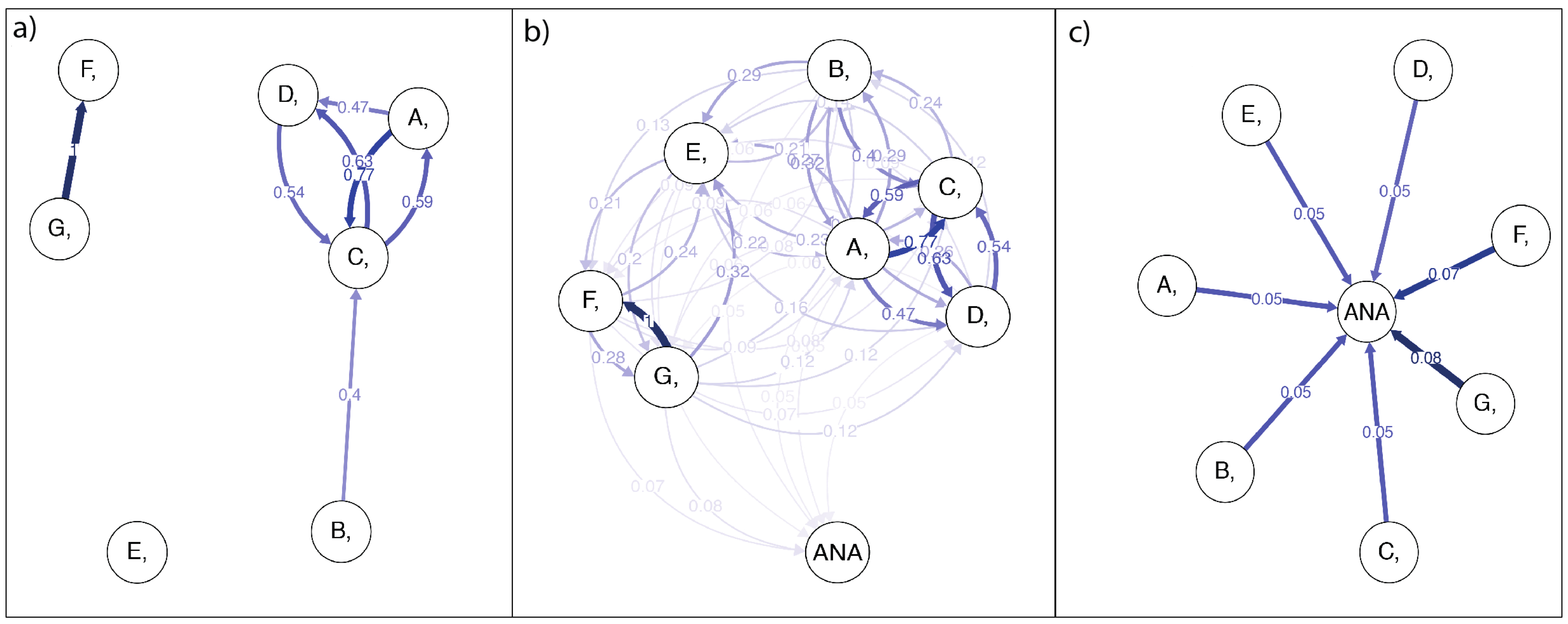
Figure 8: Directional relative migration estimated by divMigrate-online. Figure a) includes population A to G and the filter threshold is set to 0.35. In figure b) data from the anadromous salmon (ANA) is included, no filter is used. Figure c) illustrate the migration that is found to be asymmetric, no filter is used.

Estimated gene flow patterns can be visualised and explored using network graphics produced using the qgraph R package (Epskamp et al., , 2012). Population samples are represented by nodes in the networks. Each node is hypothetically connected to every other node by two connections, representing the two reciprocal gene flow components between any pair of populations. The properties of these connections, such as their length, shading and thickness are determined by the relative strength of gene flow. These properties have a particularly beneficial consequence, namely, populations that exchange genes at high rates locally, but low rates elsewhere tend to cluster together within the network space, thus providing a visual illustration of genetic structuring patterns (e.g. figure 8a below). DivMigrate-online also provides an useful filter threshold function that makes it possible to show only values above a specified number. This is a useful feature when getting to know the data set since it gives the possibility to zoom in and out, especially if many populations are compared simultaneously and the whole picture contains very much information. It can also be useful if low migration rates are not of equal interest as high ones.

The divMigrate-online application provides an integrated statistical testing facility, where the asymmetry between migration rates is tested. The statistical significance of differences between directional components of gene flow for a population pair is estimated as follows:

1. Resampling of the original data (with replacement) $x$ number of times.

2. Estimate allele frequencies from resampled data for both populations as well as their hypothetical pool of migrants

3. Calculate a user specified relevant parameter (e.g. $D$ or $G_{st}$ ) between the hypothetical pool of migrants and both populations for all $x$ resamples

4. Construct two 95% confidence intervals of the user specified parameter calculated between each population and their shared hypothetical pool of migrants using the quantile method (lower probability = 0.025, upper probability = 0.975).

5. Test for overlap of the estimated 95% confidence intervals. Where there is no overlap, the directional gene flow components are said to be significantly different (asymmetric).

This procedure can be coupled with network visualizations, such that only statistically significant asymmetric links between population pairs are plotted.

While the web application will be sufficient for most users, there may be those who require more flexibility when conducting specialized analyses (e.g. simulation studies where batches of files need to be processed). For this purpose the methods provided in divMigrate-online are also implemented in the divMigrate function from the diveRsity R package (Keenan et al., , 2013). Users interested in using this function can find out more by typing Ô?divMigrateÕ into the R console (diveRsity must be installed and loaded first).

4.2 Simulated example

Using fastsimcoal2 (Excoffier and Foll, , 2011) five populations connected in a circular stepping stone model with unidirectional migration (1$\rightarrow$2$\rightarrow$3$\rightarrow$4$\rightarrow$5$\rightarrow$1 (rate $0.0005$)) was simulated and then analyzed with divMigrate-online. For details about the simulation see (https://github.com/lisasundqvist/Sundqvist_et_al_2016).

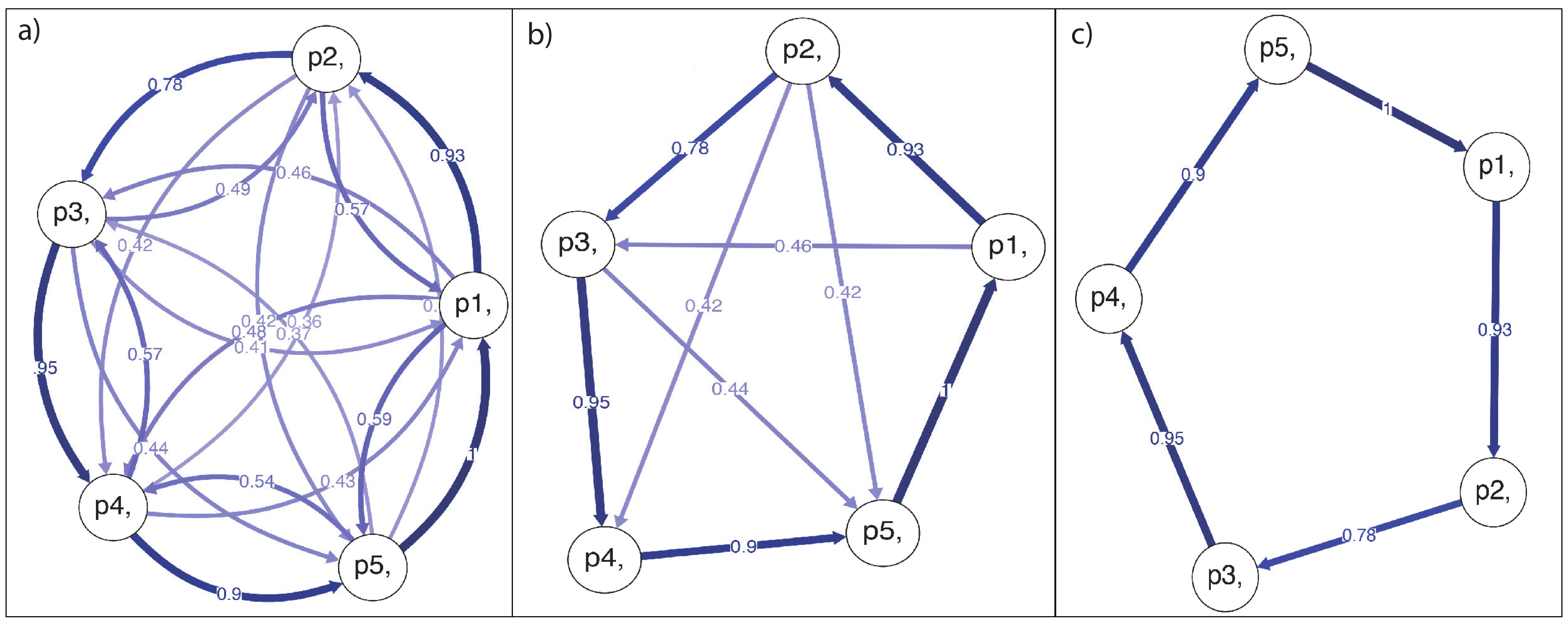
Figure 7: Directional relative migration calculated by divMigrate-online for the simulated circular stepping stone model with unidirectional migration. Figure a) illustrate the calculated migration values. Figure b) only include the values found to be asymmetric, i.e. they are statistically higher in the shown direction. In figure c) the filter threshold for the asymmetric values are set to 0.5.

Running the data set in divMigrate-online and choosing $D$ to estimate relative migration, the result, as shown in figure 7a is generated. All values except very low ones are visualized in this figure. Depending on the amount of data in the data set divMigrate-online do not always plot all values, all values are however included and can be seen in a result matrix. The result in figure 7a indicate many migration directions not simulated, this is not surprising given that the simulated migration pattern is circular and that migration between the populations occurred for many generations. Alleles can thus pass through intermediate populations and populations not directly connected can experience indirect gene flow.

To further investigate the data set, we asked divMigrate-online to estimate 1000 bootstrap iteration, and calculate confidence intervals for all values to investigate whether the migration is asymmetric. Figure 7b, only shows arrows for the directions that are statistically higher relative to the opposite direction. DivMigrate-online also provides an useful filter threshold function that makes it possible to filter out low values, thus it is easier to visualize potentially more relevant patterns. In figure 7c, the filter threshold is set to 0.5 meaning that only the asymmetric values above 0.5 are shown. In this figure, the same migration pattern that was put into the simulation is shown. All networks graphics can be exported from the application in various file formats, making the creation of publication standard plots straightforward. It is also possible to download a result matrix including all numbers.

4.3 Empirical example

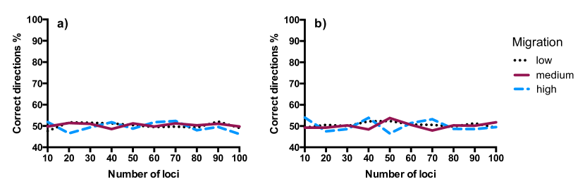
Figure 4: Bidirectional symmetric migration: percent correct directions as a function of number of loci calculated using $D$ (a) and $G_{st}$ (b). Increasing number of loci are evaluated at high ($0.05$), medium ($0.005$) and low ($0.00025$) gene flow. The sample size is kept fixed at 50. When migration is symmetric the expected value is 50%.

Recently, Sandlund et al., 2014b published a study of the spatial and temporal genetic structure of the rare landlocked salmon in a fragmented river in Norway. Using microsatellite genotype data, the authors identified three distinct genetic clusters. The first cluster contained individuals sampled from sites A, B, C and D, while the second cluster contained individuals sampled from site E, and the third cluster contained individuals sampled from sites F and G. As mentioned previously, the network method used to visualize gene flow patterns in divMigrate-online has the useful property of representing closely related population samples as local clusters within the network space. To demonstrate this the contemporary microsatellite data from the original study (Sandlund et al., 2014a, ) were re-analyzed by divMigrate-online using Josts $D$. By setting the filter threshold to 0.35 the genetic structure described in (Sandlund et al., 2014b, ) is reproduced in figure 8a. Indeed, the groups shown in figure 8a are similar to the Neighbour-joining dendrogram shown in figure 4 of (Sandlund et al., 2014b, ) (excluding the historical samples that were not included in the divMigrate-online analysis). Further, we include data of the anadromous salmon (ANA) and observe that the landlocked populations are more closely related to each other then to the anadromous salmon. In figure 8b, the result is shown with no filter. When checking for asymmetric gene flow in the system (figure 8c), an interesting result was observed, no significant asymmetry was found between the landlocked populations, but all landlocked populations exhibited asymmetric gene flow to the anadromous salmon population. Considering the history of this system, in particular the fact that these landlocked populations have been isolated from the anadromous salmon for some 9.500 years, it is likely that this pattern is showing us something else. In the definition of this method, we use private alleles or alleles only present in one population as a sign of no migration. In a system that historically has been colonized by a small number of individuals, however, it is likely that the colonized populations share many of its alleles with its source population. It is also likely that the source population displays a higher level of genetic diversity, and thus are characterized by the presence of a larger number of private alleles when compared to the colonized population. It is therefore possible that a strong and recent founder effect is the cause of what appears to be asymmetrical migration to the method. This is a particular caveat of the method described in here which potential users should be aware of.

4.4 Accessing the software

divMigrate-online is a web based software application and can be accessed on any operating system through a web browser at https://popgen.shinyapps.io/divMigrate-online/. The application can also be launched locally using R. The procedure is as follows:

1. Install the ÔshinyÕ package in R: install.packages(ÒshinyÓ)

2. Install diveRsity from github (instructions can be found at https://github.com/kkeenan02/diveRsity#development-version

3. Launch divMigrate-online: shiny::runGitHub(Òkkeenan02/divMigrate-onlineÓ)

The source code for the software is freely available at

https://github.com/kkeenan02/divMigrate-online. Pull requests can also be made through this repository.

5 Discussion

Here we have introduced a novel alternative approach that estimates directional genetic differentiation and relative migration from any relevant measure of genetic differentiation, thus allowing for the detection of asymmetric gene flow patterns. Tests using simulated data demonstrate that the new approach can detect underlying gene flow patterns with high confidence when migration is present in either one or two directions. The method performed best when gene flow was intermediate ($m=0.005$). In situations where gene flow was high ($m=0.05$), the method failed to detect underlying patterns of migration at a sufficiently high percentage for any of the sample sizes or number of loci combinations tested. The low number of times that the simulated direction was found when migration was high is likely linked to the homogenizing effect of high gene flow, resulting in very low differentiation between populations (i.e.$F_{st}\approx 0.005$). The directional components of gene flow were thus obscured (i.e. the signal to noise ratio was low). However, the upward trend for both increasing sample size and number of loci suggest that under suitable conditions the method may be capable of resolving such patterns even for cases where genetic structuring is weak.

Based on the simulation results, relative migration calculated from $G_{st}$ performed slightly better than those calculated from $D$. These results are in line with recent observations of the relative properties of $D$ and $G_{st}$ under variable demographic scenarios (Alcala et al., , 2014). Alcala et al. 2014 state that $D$ and $G_{st}$ are complementary measures, and suggest general guidelines for when the use of $G_{st}$ or $D$ might be inappropriate. For example when the expression $\theta<1<n\theta$ is true, (where $\theta$ is the scaled mutation rate ($\theta$ $=2N\mu$) and $n$ is the number of populations), as is the case in the simulations used here, the use of $G_{st}$ is recommended (table 4 in Alcala et al., 2014). Alcala et al., (2014) also introduced a new statistic for the calculation of $Nm$ (i.e. the effective number of migrants). This statistic incorporates complementary information from both $G_{st}$ and $D$, suggesting it may be a more generally suitable measure of migration. When using $Nm_{Alcala}$ for calculating the percent of correct directions in the different simulation scenarios, the result is very similar to the result obtained when using $G_{st}$. The simulation results for $Nm_{Alcala}$ is shown in Appendix 1. In divMigrate-online it is possible to calculate directional relative migration from $Nm_{Alcala}$ as well as from $D$ and $G_{st}$.

The network plots in divMigrate-online has the very useful property of representing similar population samples as local clusters within the network space. Because the directional migration calculations require that populations are pre-determined, this feature is likely to be useful only as a confirmatory complement to more quantitative methods such as those implemented in STRUCTURE (Pritchard et al., , 2000), ADEGENET (Jombart, , 2008) or DAPC (Jombart et al., , 2010). The filter threshold function makes it easy to visualize a data set, but how to filter a data set is subjective and it is therefore important to clearly state when and how this function is used.

In certain systems estimates of directional relative migration may be influenced by historic demography, as discussed in the empirical example with the landlocked Salmon. Where historical events such as founder effects or recent common ancestry have influenced the genetic composition of individuals and/or populations, footprints will be left. These footprints may enhance or diminish signs of recent migration in the genetic data. The information about migration is then obscured and makes it difficult for any method to correctly describe the migration patterns correctly. The result of the method can never reveal more information than what is to be found in the allele frequencies examined. Future work might include a more comprehensive exploration of how good the method is to detect signs of founder effects and if it is possible to distinguish them from asymmetric migration. It would also be interesting to investigate how recent common ancestry affects the ability of the method to detect contemporary migration patterns. The composition of populations may also lead to complications. In small populations fore instance genetic drift plays a bigger role. If a migrating allele is lost due to genetic drift the trace of that migration event will also be lost. If populations are uneven in size the relative impact of an allele will be different in the different populations and it will be difficult to interpret the meaning of the directional relative migration calculated, especially if one of the populations is small. By weighing the allele frequencies of populations proportionally to local size or reproductive values one could probably improve the results of the method in such situations (Hössjer et al., , 2014). In addition, it remains to be examined how robust the method is when applied to system not at equilibrium (Boileau et al., , 1992) and with influences of ghost populations (Beerli, , 2004).

When using allele frequency data, it is possible that alleles present at low frequencies are underestimated due to sampling effects (Fung and Keenan, , 2014; Gautier et al., , 2013). Since less common alleles (or alleles only present in one population) are used as an indication of no gene flow, rates estimated by the model may be slightly inflated if applied to imprecisely estimated allele frequencies. However, using alleles only present in one population as an indication of gene flow is a common strategy. Slatkin called these ”private alleles” and showed that the logarithmic average frequency of private alleles are approximately linearly related to the logarithm of $Nm$ (Slatkin, , 1985). This issue is somewhat dealt with in our model, since its focus is only on relative migration, thus, making it possible to assume that the probability of underestimating low frequency alleles is equally high in all populations.

Other available approaches for calculating asymmetric migration, such as Migrate (Beerli, , 2009) and BayesAss (Wilson and Rannala, , 2003), while powerful, are known to be difficult to use correctly, due, in part, to the large number of parameters and options that need to be adjusted to the data set under consideration. Thus, the use of these programs as black-boxes can lead to misleading results assigned a high confidence (Faubet et al., , 2007). Furthermore, these programs are also computationally demanding and, hence, can sometimes take impractical amounts of time to run. In comparison, the method presented here is easy to use, conceptually tangible and computationally efficient.

In conclusion, by introducing the concept of directional genetic differentiation, the novel method presented in here, enables users to gain new knowledge about genetic structure in systems that experience asymmetric gene flow. By acquiring such information, it is possible to examine the relationships between the direction of migration to correlated factors such as wind or water currents, which has been done in Godhe et al., (2013), Sjöqvist et al., (2015) and Godhe et al., (2015). This can lead to new insights about evolutionary processes, as well as allowing for more accurate predictions for the purposes of conservation and management. Of particular note is the utility of the method for understanding meta-populations and their source-sink dynamics. More specifically, the ability to identify low quality sink populations as well as high quality source populations is a major challenge in conservation genetics, and is readily possible using the method presented here.

6 Acknowledgements

We kindly acknowledge Per Jonsson for valuable comments on the manuscript and Anna Godhe and Kerstin Johannesson for valuable discussions. We also acknowledge helpful reviewers for valuable comments that considerably improved the paper. We are also grateful to the authors of Sandlund et al, (2014) for making their data publicly and freely available. LS was supported by the Faculty of Science at the University of Gothenburg. DK was supported by the Linnaeus Centre for Marine Evolutionary Biology at the University of Gothenburg (www.cemeb.science.gu.se) founded by a Linnaeus-grant from the Swedish Research Councils, VR and Formas. KK was supported by a Ph.D studentship from the Beaufort Marine Research Award in Fish Population Genetics, funded by the Irish Government under the Sea Change programme, the National Marine Knowledge, Research and Innovation Strategy 2007-2013. PAP was also supported by this award. KK also received support by way of a Research Award from the Department of Culture, Arts and Leisure, Northern Ireland (R3579BSC).

7 Data Accessibility

Only simulated and already published data is used in this manuscript, computer code is freely available at github repository (https://github.com/lisasundqvist/Sundqvist_et_al_2016).

8 Figures and tables

	Population A	Population B
Allele 1	$0.4$	$0.2$
Allele 2	$0.6$	$0.3$
Allele 3	$0.0$	$0.5$

¥

Table 1: Allelic matrix $A$ of the thought experiment consisting of two populations A and B with directional gene flow from A to B.

9 Appendix

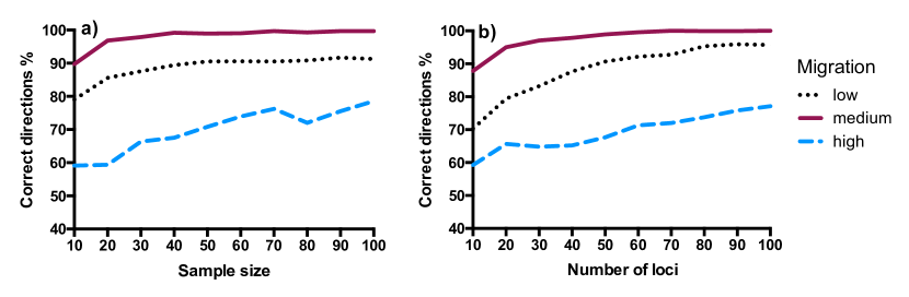
Figure A1: Unidirectional migration: percent correct directions as a function of sample size (a) and number of loci (b) calculated using $Nm_{Alcala}$. Increasing sample size and number of loci are evaluated at high ($0.05$), medium ($0.005$) and low ($0.00025$) gene flow. When sample size is evaluated the number of loci are kept fixed at 50 and when the number of loci are evaluated the sample size is kept fixed at 50.

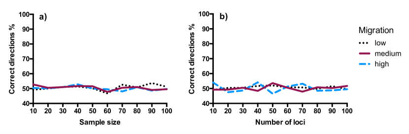
Figure A2: Bidirectional symmetric migration: percent correct directions as a function of sample size (a) and number of loci (b) calculated using $Nm_{Alcala}$. Increasing sample size and number of loci are evaluated at high ($0.05$), medium ($0.005$) and low ($0.00025$) gene flow. When sample size is evaluated the number of loci are kept fixed at 50 and when the number of loci are evaluated the sample size is kept fixed at 50. When migration is symmetric the expected value is 50%.

Figure A3: Bidirectional asymmetric migration: percent correct directions as a function of sample size (a) and number of loci (b) calculated using $Nm_{Alcala}$. Increasing sample size and number of loci are evaluated at high ($0.05$), medium ($0.005$) and low ($0.00025$) gene flow. When sample size is evaluated the number of loci are kept fixed at 50 and when the number of loci are evaluated the sample size is kept fixed at 50.

References

- Alcala et al., (2014) Alcala, N., Goudet, J., and Vuilleumier, S. (2014). On the transition of genetic differentiation from isolation to panmixia: What we can learn from gst and d. Theoretical population biology, 93:75–84.
- Beerli, (2004) Beerli, P. (2004). Effect of unsampled populations on the estimation of population sizes and migration rates between sampled populations. Molecular Ecology, 13(4):827–836.
- Beerli, (2009) Beerli, P. (2009). How to use migrate or why are markov chain monte carlo programs difficult to use. Population genetics for animal conservation, 17:42–79.
- Bhargava and Fuentes, (2010) Bhargava, A. and Fuentes, F. (2010). Mutational dynamics of microsatellites. Molecular biotechnology, 44(3):250–266.
- Boileau et al., (1992) Boileau, M. G., Hebert, P. D. N., and Schwartz, S. S. (1992). Non-equilibrium gene frequency divergence: persistent founder effects in natural populations. Journal of Evolutionary Biology, 5(1):25–39.
- Cowen and Sponaugle, (2009) Cowen, R. K. and Sponaugle, S. (2009). Larval dispersal and marine population connectivity. Annual Review of Marine Science, 1:443–466.
- Crawford, (2010) Crawford, N. G. (2010). Smogd: software for the measurement of genetic diversity. Molecular Ecology Resources, 10(3):556–557.
- Dias, (1996) Dias, P. (1996). Sources and sinks in population biology. Trends in Ecology & Evolution, 11(8):326–330.
- Eddelbuettel et al., (2011) Eddelbuettel, D., François, R., Allaire, J., Chambers, J., Bates, D., and Ushey, K. (2011). Rcpp: Seamless r and c++ integration. Journal of Statistical Software, 40(8):1–18.
- Epskamp et al., (2012) Epskamp, S., Cramer, A. O., Waldorp, L. J., Schmittmann, V. D., and Borsboom, D. (2012). qgraph: Network visualizations of relationships in psychometric data. Journal of Statistical Software, 48(4):1–18.
- Excoffier and Foll, (2011) Excoffier, L. and Foll, M. (2011). Fastsimcoal: a continuous-time coalescent simulator of genomic diversity under arbitrarily complex evolutionary scenarios. Bioinformatics, 27(9):1332–1334.
- Faubet et al., (2007) Faubet, P., Waples, R. S., and Gaggiotti, O. E. (2007). Evaluating the performance of a multilocus bayesian method for the estimation of migration rates. Molecular Ecology, 16(6):1149–1166.
- Friedman and Barrett, (2009) Friedman, J. and Barrett, S. C. (2009). Wind of change: new insights on the ecology and evolution of pollination and mating in wind-pollinated plants. Annals of Botany, 103(9):1515–1527.
- Fung and Keenan, (2014) Fung, T. and Keenan, K. (2014). Confidence intervals for population allele frequencies: The general case of sampling from a finite diploid population of any size. PloS one, 9(1):e85925.
- Gautier et al., (2013) Gautier, M., Foucaud, J., Gharbi, K., Cézard, T., Galan, M., Loiseau, A., Thomson, M., Pudlo, P., Kerdelhué, C., and Estoup, A. (2013). Estimation of population allele frequencies from next-generation sequencing data: pool-versus individual-based genotyping. Molecular Ecology, 22(14):3766–3779.
- Godhe et al., (2013) Godhe, A., Egardt, J., Kleinhans, D., Sundqvist, L., Hordoir, R., and Jonsson, P. R. (2013). Seascape analysis reveals regional gene flow patterns among populations of a marine planktonic diatom. Proceedings of the Royal Society of London B: Biological Sciences, 280(1773):20131599.
- Godhe et al., (2015) Godhe, A., Sjöqvist, C., Sildever, S., and Lundholm, N. (2015). Physical barriers and environmental gradients cause spatial and temporal genetic differentiation of an extensive algal bloom. Journal of Biogeography.
- Hänfling and Weetman, (2006) Hänfling, B. and Weetman, D. (2006). Concordant genetic estimators of migration reveal anthropogenically enhanced source-sink population structure in the river sculpin, cottus gobio. Genetics, 173(3):1487–1501.
- Hedrick and Goodnight, (2005) Hedrick, P. W. and Goodnight, C. (2005). A standardized genetic differentiation measure. Evolution, 59(8):1633–1638.
- Hössjer et al., (2014) Hössjer, O., Olsson, F., Laikre, L., and Ryman, N. (2014). A new general analytical approach for modeling patterns of genetic differentiation and effective size of subdivided populations over time. Mathematical biosciences, 258:113–133.
- Jombart, (2008) Jombart, T. (2008). adegenet: a r package for the multivariate analysis of genetic markers. Bioinformatics, 24(11):1403–1405.
- Jombart et al., (2010) Jombart, T., Devillard, S., and Balloux, F. (2010). Discriminant analysis of principal components: a new method for the analysis of genetically structured populations. BMC genetics, 11(1):94.
- Jost, (2008) Jost, L. (2008). GST and its relatives do not measure differentiation. Molecular Ecology, 17(18):4015–4026.
- Keenan et al., (2013) Keenan, K., McGinnity, P., Cross, T. F., Crozier, W. W., and Prodöhl, P. A. (2013). diversity: An r package for the estimation and exploration of population genetics parameters and their associated errors. Methods in Ecology and Evolution, 4(8):782–788.
- Meirmans and Hedrick, (2011) Meirmans, P. and Hedrick, P. (2011). Assessing population structure: FST and related measures. Molecular Ecology Resources, 11(1):5–18.
- Muñoz et al., (2004) Muñoz, J., Felicísimo, Á. M., Cabezas, F., Burgaz, A. R., and Martínez, I. (2004). Wind as a long-distance dispersal vehicle in the southern hemisphere. Science, 304(5674):1144–1147.
- Nei, (1973) Nei, M. (1973). Analysis of gene diversity in subdivided populations. Proceedings of the National Academy of Sciences, 70(12):3321–3323.
- Paz-Vinas et al., (2013) Paz-Vinas, I., Quéméré, E., Chikhi, L., Loot, G., and Blanchet, S. (2013). The demographic history of populations experiencing asymmetric gene flow: combining simulated and empirical data. Molecular Ecology, 22(12):3279–3291.
- Pringle et al., (2011) Pringle, J. M., Blakeslee, A. M., Byers, J. E., and Roman, J. (2011). Asymmetric dispersal allows an upstream region to control population structure throughout a species? range. Proceedings of the National Academy of Sciences, 108(37):15288–15293.
- Pritchard et al., (2000) Pritchard, J. K., Stephens, M., and Donnelly, P. (2000). Inference of population structure using multilocus genotype data. Genetics, 155(2):945–959.
- (31) Sandlund, O., Karlsson, S., Thorstad, E., Berg, O., Kent, M., Norum, I., and Hindar, K. (2014a). Data from: Spatial and temporal genetic structure of a river-resident atlantic salmon (salmo salar) after millennia of isolation.
- (32) Sandlund, O. T., Karlsson, S., Thorstad, E. B., Berg, O. K., Kent, M. P., Norum, I. C., and Hindar, K. (2014b). Spatial and temporal genetic structure of a river-resident atlantic salmon (salmo salar) after millennia of isolation. Ecology and evolution, 4(9):1538–1554.
- Siegel et al., (2003) Siegel, D., Kinlan, B., Gaylord, B., and Gaines, S. (2003). Lagrangian descriptions of marine larval dispersion. Marine Ecology Progress Series, 260:83–96.
- Sjöqvist et al., (2015) Sjöqvist, C., Godhe, A., Jonsson, P., Sundqvist, L., and Kremp, A. (2015). Local adaptation and oceanographic connectivity patterns explain genetic differentiation of a marine diatom across the north sea–baltic sea salinity gradient. Molecular ecology, 24(11):2871–2885.
- Slatkin, (1985) Slatkin, M. (1985). Rare alleles as indicators of gene flow. Evolution, pages 53–65.
- Whitlock and McCauley, (1999) Whitlock, M. C. and McCauley, D. E. (1999). Indirect measures of gene flow and migration: Fst 1/(4nm+ 1). Heredity, 82(2):117–125.
- Wilson and Rannala, (2003) Wilson, G. and Rannala, B. (2003). Bayesian inference of recent migration rates using multilocus genotypes. Genetics, 163(3):1177–1191.
- Wright, (1931) Wright, S. (1931). Evolution in mendelian populations. Genetics, 16(2):97.
- Wright, (1943) Wright, S. (1943). Isolation by distance. Genetics, 28(2):114.
- Wright, (1949) Wright, S. (1949). The genetical structure of populations. Annals of Human Genetics, 15(1):323–354.