Minimal Model for Stem-Cell Differentiation

Abstract

To explain the differentiation of stem cells in terms of dynamical systems theory, models of interacting cells with intracellular protein expression dynamics are analyzed and simulated. Simulations were carried out for all possible protein expression networks consisting of two genes under cell–cell interactions mediated by the diffusion of a protein. Networks that show cell differentiation are extracted and two forms of symmetric differentiation based on Turing’s mechanism and asymmetric differentiation are identified. In the latter network, the intracellular protein levels show oscillatory dynamics at a single-cell level, while cell-to-cell synchronicity of the oscillation is lost with an increase in the number of cells. Differentiation to a fixed-point type behavior follows with a further increase in the number of cells. The cell type with oscillatory dynamics corresponds to a stem cell that can both proliferate and differentiate, while the latter fixed-point type only proliferates. This differentiation is analyzed as a saddle-node bifurcation on an invariant circle, while the number ratio of each cell type is shown to be robust against perturbations due to self-consistent determination of the effective bifurcation parameter as a result of the cell–cell interaction. Complex cell differentiation is designed by combing these simple two-gene networks. The generality of the present differentiation mechanism, as well as its biological relevance, is discussed.

I Introduction

The differentiation of multipotent stem cells into lineage-specific cells is an important process in developmental biology, for which an understanding in terms of dynamical systems theory is desired. Stem cells can both proliferate (i.e., reproduce themselves) and differentiate into other cell types Lenza ; Potten ; Melton ; Slack . While the former indicates that the cellular state is stable in retaining its composition, the latter implies that the original cellular state is also unstable in that it moves toward a state with different compositions. How a stem cell simultaneously supports these two conflicting features is an important question.

Dynamical system approaches to cell differentiation have been developed by considering that abundances of cellular components are changed through intracellular reactions Waddington ; Newman ; Goodwin ; Glass ; Kauffman ; Kauffman2 ; Huang . Protein expression dynamics consist of mutual activation and inhibition, and the concentration of each protein changes over time, while its composition determines the cellular state. A dynamical system in the state space that consists of each protein expression level can then be considered. Based on this picture, it is natural to assign an attractor to each cell type, which allows the robustness of each cell type to be explained as the stability of an attractor against noise. If the system has multiple attractors, each differentiated cell type corresponds to each attractor.

Although this attractor picture is important for understanding the robustness of each cellular state and how distinct cell types are formed, answers to the following questions remain elusive: (i) Which attractor describes the two conflicting functions in stem cells, i.e., proliferation and differentiation? (ii) How are initial conditions for different attracting states selected through the course of development? (iii) How is the stability of the developmental course, i.e., the robustness in the timing of cell differentiation, and the number distribution of each cell explained, which possibly includes regulation of the cell–cell interactions?

To address these questions, coupled dynamical systems that include intracellular dynamics of protein abundances, cell–cell interaction, and an increase in the cellular number by cell division were developed KK-Yomo94 ; KK-Yomo97 ; KK-Yomo99 ; Furusawa-KK98 ; Furusawa-KK01 . Cells with oscillatory intracellular dynamics of protein concentrations were shown to differentiate to a novel type with an increase in the cell number, and a cell model whose protein expressions are regulated by a gene regulatory network (GRN) with 5 genes has recently been studied SFK . From extensive simulations, GRNs that include “stem cells” that can undergo both proliferation and differentiation were selected. The cells always exhibited oscillatory expression dynamics as a single-cell level, and after divisions, synchronization of the oscillations among cells was lost. With further cell division, differentiation to a cell type that loses the oscillatory expression followed. Furthermore, it is interesting to note that recent measurements of protein expression dynamics in embryonic stem cells support this oscillation scenario Kobayashi . The importance of intracellular oscillation to cell differentiation is now being recognized in the developmental biology community Furusawa-KK12 .

To analyze this differentiation mechanism in terms of dynamical systems theory, however, it would be useful to adopt a simpler system consisting of fewer genes. Here, we study such a minimal system, i.e., dynamical systems consisting of expression levels of only two genes (proteins). After introducing the model in §II, we describe the results in §III. By simulating all possible regulation networks consisting of two proteins with various parameters, we extract a minimal system that allows for stem-cell differentiation. In such a system, the protein expression levels oscillate in time as a single-cell level. With an increase in the cell number, synchronization in the oscillation among cells is lost due to cell–cell interactions and some cells then differentiate to fall into fixed-point dynamics losing the oscillation. This process is analyzed using bifurcation theory and explained in terms of a saddle-node on an invariant circle (SNIC) bifurcation. We also show that the number of each cell type after development is robust against noise. The extracted two-gene network leading to the SNIC is shown to provide a universal motif for asymmetric differentiation from stem cells, while complex hierarchical differentiation is designed by simply combining the extracted two-gene network in parallel or in sequence. The relevance of the present results to dynamical systems and biological cell differentiation is discussed briefly in §IV.

II Model

II.1 Intracellular protein expression dynamics

Here we describe our cell differentiation model under cell-to-cell interactions. Cell states are represented by protein expression levels of two genes $x$ and $y$. These $x$ and $y$ genes can regulate the protein expression level of both itself and the other gene. We consider the dynamics of the expression levels (protein concentrations) of the two proteins, denoted as $x_{i}(t)$ and $y_{i}(t)$, of the $i$-th cell at time $t$. Following earlier studies, we eliminate the mRNA concentration synthesized from each gene and obtain the dynamical system only of the protein expression levels. The dynamics of the expression levels at a single cell are described as

$$\begin{split}\frac{dx_{i}(t)}{dt}=\frac{1}{1+exp\{-\beta(J_{xx}x_{i}(t)+J_{xy}y_{i}(t)-g_{x})\}}-x_{i}(t)\\ \frac{dy_{i}(t)}{dt}=\frac{1}{1+exp\{-\beta(J_{yx}x_{i}(t)+J_{yy}y_{i}(t)-g_{y})\}}-y_{i}(t).\\ \end{split}$$ (1)

The $2\times 2$ matrix $J_{m\ell}$ ($m,\ell=x,y$) gives the transcriptional regulation from protein $\ell$ to $m$, where $J_{m\ell}=1$ if the gene $\ell$ activates the expression of $m$, $-1$ if it inhibits the expression, and 0 if there is no regulation. A sigmoid function of the form $exp(-\beta(z-g))$ is adopted gene-net to represent the on–off type expression with $\beta$ as the sensitivity parameter, which roughly corresponds to the Hill coefficient in terms of cell biology, where for $\beta\rightarrow\infty$ the function approaches the step function. The parameters $g_{x}$ and $g_{y}$ give the threshold values of the expressions of the $x$ and $y$ genes, respectively.

II.2 Cell–cell interaction

The cells interact with each other and this interaction is mediated by some signal. We assume here that the interaction is mediated directly or indirectly by one of the proteins, which we take to be $y$. In its simplest form, we consider only the interaction by the diffusion of the $y$ protein. By assuming that the diffusion is fast and by discarding spatial inhomogeneity over the cells, we employ global coupling, i.e., an all-to-all mean-field interaction. Thus, the overall gene expression dynamics obey the following equation:

$$\begin{split}\frac{dx_{i}(t)}{dt}=\frac{1}{1+exp\{-\beta(J_{xx}x_{i}(t)+J_{xy}y_{i}(t)-g_{x})\}}-x_{i}(t)\\ \frac{dy_{i}(t)}{dt}=\frac{1}{1+exp\{-\beta(J_{yx}x_{i}(t)+J_{yy}y_{i}(t)-g_{y})\}}-y_{i}(t)+\\ \frac{D}{N(t)}(\sum_{k=1}^{N}y_{k}(t)-y_{i}(t)),\\ \end{split}$$ (2)

where $D$ is the diffusion constant, and $N(t)$ is the total number of cells at time $t$.

II.3 Cell division

To examine the cell differentiation process through development, the number of cells $N(t)$ is increased over time by cell division. Starting with a single cell, this cell is divided into two cells that have almost the same protein concentrations at a certain time. The concentrations $x_{i}(t)$ and $y_{i}(t)$ are slightly perturbed by cell division, leading to cell differences that obey a Gaussian distribution with the variance $\sigma$, which is set sufficiently small. Here, the behavior to be discussed (i.e., whether cell differentiation appears) is independent of the noise level. Noise is included mainly to remove synchronization over cells, which is unstable but preserved due to numerical computation with a finite bit. The cells are simply divided into two after every time span $t_{d}$.

II.4 Model parameters and criterion for differentiation

To numerically investigate this model, we set the sensitivity parameter as $\beta=40$ and the division noise level as $\sigma=10^{-3}$. The results do not depend on these specific values, as long as the former is sufficiently large (e.g., $\beta>5$) and the latter is not too large (e.g., $\sigma<0.1$). The division time $t_{d}$ is chosen to be 25, but this specific value also does not affect the results.

We scanned the other parameters for all possible choices of $J_{m\ell}=\pm 1,0$ ($m,\ell=x$ or $y$) to examine the possibility of cell differentiation. We also checked all possible configurations of $J_{m\ell}$ as long as the matrix includes at least one off-diagonal component (i.e., as a minimum, the interaction between $x$ and $y$ exists). This gives a total of 36 configuration. The parameters $g_{x,y}$ were varied from $-1$ to 1 in increments of 0.05, and $D$ was chosen as either 0.2 or 1.0. Thus, the model in Eq.(2) was simulated for a total of $36\times 41\times 41\times 2=121032$ cases.

To examine if cells differentiated, we increased the cell population to $N=32$. For each cell, we computed the temporal average of the gene expression level for a sufficiently long time after discarding the transient time. If the difference between the maximum and minimum averaged gene expression levels ($x_{i}(t)$, $y_{i}(t)$) over the cells was larger than 0.1, then we concluded that differentiation had occurred.

III Results

III.1 Differentiation classification

Type	Behavior	Network	Parameter
Turing	fixed point  $\rightarrow$ fixed point	2/36	6/121032
Oscillation death	oscillation  $\rightarrow$ fixed point	2/36	3/121032
Asymmetric differentiation	oscillation$\rightarrow$
with oscillation	oscillation	2/36	9/121032

The simulation results revealed cell differentiation cases that can be classified into the following three types: 1) Turing, 2) Oscillation death, and 3) Asymmetric differentiation with remnant oscillations. In all cases, the single-cell dynamics had only a single attractor. As the cell number increases, the cells take two distinct states. We first describe these three types and show that the mechanisms of the first two types are already well known. We thus focus on the third type, which is the most relevant to differentiation of stem cells.

III.1.1 Turing type (fixed point$\rightarrow$fixed point)

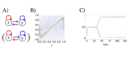
Fig. 1: (a) Upper: Network structure of a model that shows Turing-type differentiation; fixed point $\rightarrow$ fixed point. Lower: The conjugate network form. The parameter values that show this differentiation are $(D,g_{x},g_{y})=(0.2,0,0),(1,0,0),(1,0.05,0.05),(1,-0.05,-0.05)$ for the upper network and $(D,g_{x},g_{y})=(0.2,1,-1),(1,1,-1),(1,0.95,-0.95)$ for the lower network. (The flow in the state space and the nullcline is simply a mirror symmetry with regard to $x=y$ in the model here and is not shown). (b) The single-cell nullcline of the model. (c) Time series of the protein expression $x_{i}(t)$ as the cell number increases from $i=1$ to 32 through cell division every 25 time units; (b) and (c) are drawn for the upper network structure with the parameter values $(D,g_{x},g_{y})=(0.2,0,0)$.

The single-cell dynamics in this case has a unique stable fixed point. As the cell number increases, the cell population splits into two groups, each taking different fixed-point values of $x$ and $y$ and a higher value of $x$ or $y$. The numbers in each population are equal, i.e., 16 cells each for $N=32$. One gene expression network type is shown in Fig. 1, where one gene activates the expression of itself and the other, while the other gene, which is diffusible, inhibits the expression of itself and the other. This mechanism is explained well by the classic Turing pattern Turing by replacing the spatially local diffusive interaction therein with global coupling. Indeed, Turing’s seminal paper included the present case, as he discussed the case with $N=2$ (see also Sano ). The conjugate network is also shown in Fig. 1 (in parentheses), where the differentiation mechanism is understood in the same way.

III.1.2 Oscillation death (oscillation $\rightarrow$ fixed point)

The single-cell dynamics for this type of differentiation has a limit-cycle attractor. With an increase in cell number, the cell population again splits into two groups of equal number, each of which shows distinct fixed points through the cell-to-cell interaction, in the same manner as the Turing-pattern case. This loss of oscillation is known as oscillation death Turing ; Prigogine ; oscillation-death ; Koseska . Two forms of the networks that show this behavior are shown in Fig. 2. The mechanism of this type of differentiation will be explained later, as it is common to that of asymmetric differentiation in the next section.

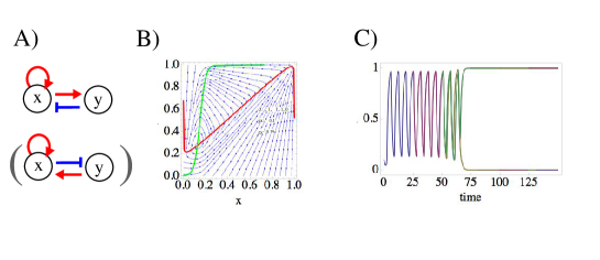
Fig. 2: (a) Upper: Network structure of a model that shows differentiation through oscillation death; oscillation $\rightarrow$ fixed point. Lower: The conjugate network form. The parameter values that show this differentiation are $(D,g_{x},g_{y})=(1,-0.1,0.15),(1,0.1,085)$ for the upper network and $(D,g_{x},g_{y})=(1,0.9,-0.15)$ for the lower network. (The flow in the state space and the nullcline is simply a mirror symmetry with regard to $x=y$ in the model here and is not shown). (b) The single-cell nullcline of the model. (c) Time series of the protein expression $x_{i}(t)$ as the cell number increases from $i=1$ to 32 through cell division every 25 time units; (b) and (c) are drawn for the upper network structure with the parameter values $(D,g_{x},g_{y})=(1,-0.1,0.15)$.

III.1.3 Asymmetric differentiation with remnant oscillation (oscillation $\rightarrow$ oscillation transition)

In this class, the attractor of a single cell is again a limit cycle, but as the number of cells is increased, synchronized oscillation over cells is unstable under the cell–cell interaction, and protein-expression oscillations are desynchronized between some cells GCM . After this desynchronization, some cells leave the original limit-cycle trajectory and enter an oscillatory state with a tiny amplitude, while the other cells remain in the original limit cycle (with a slight modification) Meinhardt . The states mutually stabilize their existence, e.g., if all the cells in one state were removed, some of the remaining cells will make a transition to the other state. Thus, two distinct oscillatory states coexist independently of the initial condition of the cells.

This class of behavior is observed for the two networks, shown in Fig. 3, over 9 sets of parameter values. The parameter interval in which the present behavior is observed is relatively small compared with the previous two cases.

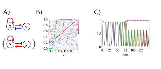
Fig. 3: (a) Upper: Network structure of a model that shows asymmetric differentiation with remnant oscillation; oscillation $\rightarrow$ oscillation transition. Lower: The conjugate network form. The parameter values that show this differentiation are $(D,g_{x},g_{y})=(0.2,-0.1,0.15),(0.2,-0.1,0.2),(0.2,-0.1,-0.25)$ for the upper network and $(D,g_{x},g_{y})=(0.2,0.1,0.75),(0.2,0.1,0.8),(0.2,0.1,0.85)$ for the lower network. (The flow in the state space and the nullcline is simply a mirror symmetry with regard to $x=y$ in the model here and is not shown). (b) The single-cell nullcline of the model. (c) Time series of the protein expression $x_{i}(t)$ as the cell number increases from $i=1$ to 32 through cell division every 25 time units; (b) and (c) are drawn for the upper network structure with the parameter values $(D,g_{x},g_{y})=(0.2,-0.1,0.2)$.

III.2 Mechanism of oscillatory differentiation

We note that none of the cells in the first two classes have the potential to both proliferate (reproduce the same type by division) and differentiate (switch to a cell type with distinct behavior). Furthermore, the first two mechanisms are already well understood based on Turing’s study, while the latter mechanism, which corresponds to the cell-differentiation mechanism in our earlier studies, is not fully understood in terms of dynamical systems theory. Hence, we focus here on the third class and explain the mechanism of the differentiation into two states.

The differentiation is based on two stages: desynchronization of the oscillations and SNIC bifurcation induced by cell-to-cell interactions SNIC ; SNIC2 . Examining the nullcline of the single-cell dynamics, shown in Fig. 4, we see that while the two nullclines come close, they do not intersect. Thus, there are no fixed points, and the limit-cycle attractor exists as a single-cell level, as already mentioned. (For the following numerical simulations, we have used the parameter values $g_{x}=-0.1$, $g_{y}=0.2$, and $D=0.14$).

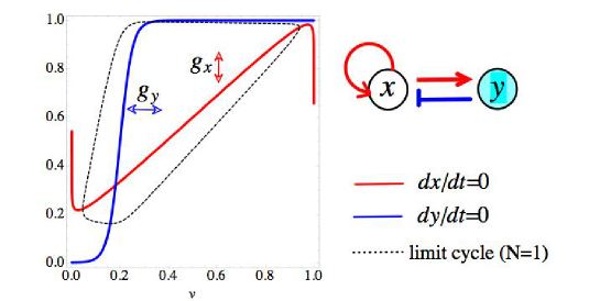
Fig. 4: The nullcline and limit-cycle attractor of the single-cell dynamics for the GRN in Fig. 3. The network is redrawn for reference, where the parameter values are $J_{xx}=1,J_{xy}=-1,J_{yx}=1,J_{yy}=0,g_{x}=-0.1,g_{y}=0.2$. The two nullclines for $dx/dt=0$ and $dy/dt=0$ are drawn in red and blue, respectively. The limit-cycle attractor is drawn as the dashed line. The two nullclines come close but do not intersect, which is an important property for differentiation to occur by cell–cell interaction. Indeed, the nullclines and the limit cycle are arranged in the same manner for the conjugate network (shown in parentheses of Fig. 3a).

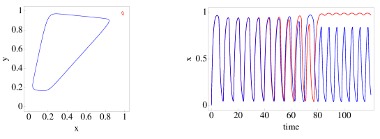
Fig. 5: Dynamics of the model in Figs. 3 and 4 with $D=0.14$. (a) Locus of the orbit of the two-cell dynamics of $(x_{(}t),y_{1}(t))$ and $(x_{2}(t),y_{2}(t))$. Blue: cell type whose state is close to the original limit cycle. Red: differentiated type with loss of autonomous oscillation. (b) The time series of $x_{i}(t)$ for the two-cell dynamics ($i=1,2$). The oscillations of the two cells are first desynchronized and at around $t\sim 80$, they split into two distinct steady states.

III.2.1 Desynchronization

Consider a coupled system with cell-to-cell interaction, where each cell shows a limit-cycle oscillation as shown above. As is known, the oscillations of the cells lose synchronization for a certain range of the interaction and parameter values. This desynchronization occurs in the present case, as was numerically confirmed by computing the stability exponent for the synchronization. Indeed, the magnitude of the tangential vector representing the deviation between the two cells $\delta{\bf X}$=($\delta x,\delta y)$ increases exponentially over time.

III.2.2 Differentiation

After desynchronization, the cell-to-cell interaction leads to differentiation with an increase in the cell number. Here, the cell–cell interaction term that occurs through diffusion in our model is represented by $\alpha(t)\equiv D(\frac{1}{N}\sum_{k=1}^{N}y_{k}-y_{i})=D(\overline{y}-y_{i})$, so that the dynamics are written as

$$\begin{split}\frac{dx(t)}{dt}=\frac{1}{1+exp\{-\beta(x(t)-y(t)-g_{x})\}}-x(t)\\ \frac{dy(t)}{dt}=\frac{1}{1+exp\{-\beta(x(t)-g_{y})\}}-y(t)+\alpha.\\ \end{split}$$ (3)

If the oscillations are synchronized over cells, then $\alpha\equiv 0$, and the equation is reduced to single-cell dynamics. Due to the desynchronization, however, $\alpha$ is nonzero and functions as a time-dependent bifurcation parameter. We first examine the bifurcation of the single-cell dynamics against changes in the constant parameter $\alpha$ and then discuss the time dependence of $\alpha$.

The nullclines of Eq. (2) are shown in Fig. 6. As $\alpha$ is changed, only the nullcline $dy/dt=0$ moves vertically downward with a decrease in $\alpha$ without a change in form; there is no effect on the nullcline $dx/dt=0$. The two nullclines intersect with a slight decrease in $\alpha$, so that the SNIC SNIC ; SNIC2 appears, and the limit-cycle attractor is replaced by a stable fixed point. (In the example in Fig. 6, this bifurcation occurs at $\alpha_{c}\approx-0.017$). In the case in which $\overline{y}$, i.e., the average of $y$ over $\alpha$, is represented as a constant value that can deviate from $y_{i}(t)$, the nullcline for $dy/dt=0$ is represented by $y=y_{c}=1/\{(1+exp\{-\beta(x-g_{y})\})(1+D)\}-D\overline{y}$ and it decreases if $D$ increases. Recalling that the $x$ nullcline $y=x+\frac{1}{\beta}log(1-1/x)-g_{x}\approx 1$ in the region near$x=1$(see figure), $x$ and $y$ nullcline intersect and a fixed point appears via the SNIC, if $D$ is large enough. In the differentiation of two cells that originates in desynchronization, as shown in Fig. 5, one cell has a larger $y_{i}$ value, and the $\alpha$ $(<0)$ value of that cell is smaller and can be smaller than $\alpha_{c}$. The nullcline $dy/dt=0$ for such a cell then intersects the nullcline $dx/dt=0$. In contrast, the other cell remains close to the original limit cycle. The effective $\alpha_{1,2}$ estimated from the diffusion term, shown in Fig. 7, demonstrates that $\alpha_{2}$ remains in the region of the fixed point($\alpha<\alpha_{c}$), which supports this argument. Thus, for a certain parameter region, the two types of behavior are differentiated: one is close to the original limit cycle and the other is close to the fixed point generated by the SNIC.

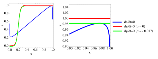
Fig. 6: (a) Change in the nullcline of $dy/dt=0$ as $\alpha$ in Eq. (3) changes. As $\alpha$ is decreased, the nullcline $dy/dt=0$ moves downwards (from the red to green line) and touches the nullcline of $dx/dt=0$ (blue), when $\alpha=-0.017$. The SNIC then follows. Details are shown in (b).

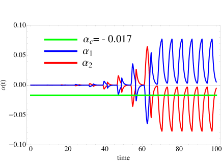
Fig. 7: Time series of the diffusion terms $D(y_{2}(t)-y_{1}(t))$ (blue) and $D(y_{1}(t)-y_{2}(t))$ (red) of the two cells. The cell–cell interaction induces desynchronization, and the difference between the cells is amplified. One cell then stays in the region of the fixed point. For reference, the value $\alpha_{c}=-0.017$ is plotted. Note that $D(y_{1}(t)-y_{2}(t))$ remains below $\alpha_{c}$ for most of the time, while $D(y_{2}(t)-y_{1}(t))$ remains above it.

Since the variables $x$ and $y$ oscillate in time, this argument assuming a constant $\alpha$ is insufficient. Still, on average, the trajectory of the differentiated cells that take a larger $y$ value remains above the nullcline $dy/dt=0$ in the state space $(x,y)$. Although the trajectory stays around the intersection of the two nullclines, the state of this cell is not completely a fixed point due to the interaction term with the other cell: since the other cell type keeps the oscillatory dynamics close to the original limit cycle, the differentiated cell type is driven by this oscillatory dynamics so that it shows an oscillation with a tiny amplitude. The original and differentiated cell types are distinguished by the ability for autonomous oscillation. Note that oscillation death(case2) is understood similary as the asymmetric differentiation. In thats case, SNIC bifurcation occur at two points around $(x,y)=(0,0)$ and $(1,1)$ on $x$-$y$ plane, and the limit cycle is replaced by the two fixed points as a result.

III.2.3 Parameter dependence

Since the desynchronization and differentiation are due to the interaction, the dynamics of the two cells depends strongly on the diffusion coefficient $D$. By taking a two-cell system with a fixed $g_{x,y}$ as above, we can examine the dependence of the two-cell dynamics on the value of $D$. In Fig. 8, the local maxima $x_{i}(t)$ of the two cells $i=1,2$ during the steady state (either a fixed point or periodic oscillation) are plotted over time. For small $D$, i.e., for weak cell–cell interaction, the oscillations of the two cells are synchronized. With an increase in $D$, the synchronization loses stability, and the oscillations desynchronize (Fig. 8); coexistence of the two oscillations occurs for larger $D$.

The corresponding changes in the time series and trajectories in $(x,y)$ space are shown for each region (A1, A2, …, A5) in Fig. 9. From A1 to A2, a period-doubling bifurcation causes the oscillations of the two cells to be out of phase. From A2 to A3 a pitchfork bifurcation occurs. Then, the period-doubling cascade to chaos appears from A3 to A4, where the two oscillations are chaotic with desynchronization. At the transition from A4 to A5, chaotic orbit touches with saddle, and crisis occurs. The chaotic orbit in the four dimensional space with two cells becomes unstable and is replaced by two stable periodic orbits. Each of the oscillations is now periodic; one with a large amplitude close to the original limit cycle and the other with a tiny amplitude near the fixed point. Form the view point of single cell dynamics, it can be regarded as occurrence of SNIC bifurcation, when we regard diffusion term as time dependent parameter. In region A5, the asymmetric differentiation from the stem-type cell, which was discussed earlier, occurs. We also note that the bifurcation in the case of oscillation death follows almost the same sequence as the present case.

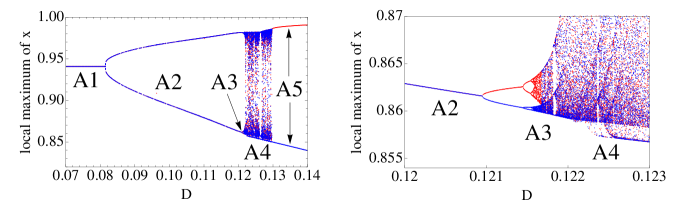
Fig. 8: Bifurcation diagram of the two-cell dynamics. (a) Local maxima of $x_{i}(t)$ for two cells ($i=1,2$; red and blue) plotted at the steady state (attractor). (b) Details around the A3-A4 transition. As $D$ is increased, the single-cell orbit is destabilized ($A1\rightarrow A2$), and the two cells take different orbits through the pitchfork bifurcation (A2). Chaos appears through the period-doubling cascade (A3) and two chaotic orbits merge so that the two cells fall into the same chaotic orbit, keeping desynchronization. With a further increase in $D$, distinct cells with different oscillations coexist (A5).

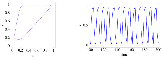
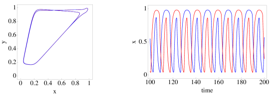
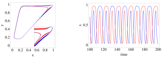
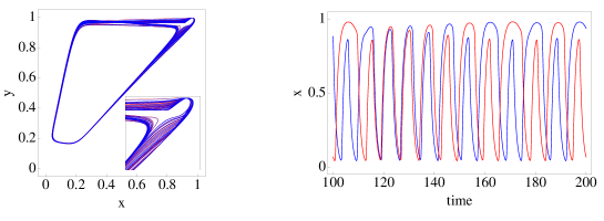
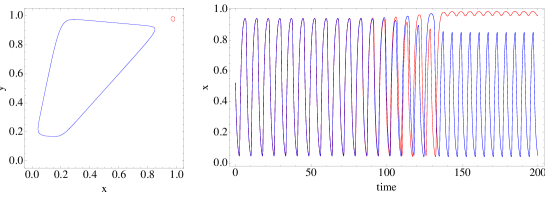
Fig. 9: Orbit and time series of the two cells. Left: Orbits of $(x_{i}(t),y_{i}(t))$ ($i=1,2$) after the cells reach a steady state (attractor). Right: The time series of $x_{i}(t)$. The colors correspond to the two different cells $i=1,2$. (i) $D=0.0$ corresponding to A1 in Fig. 8. The orbits of the two cells are synchronized. (ii) $D=0.12$ corresponding to A2. The orbits are desynchronized. (iii) $D=0.1216$ corresponding to A3. The orbits of the two cells are desynchronized and take different loci. (iv) $D=0.1225$ corresponding to A4. The two cells show chaotic dynamics and are desynchronized, while as a whole they are on the same attractor. (v) $D=0.132$ corresponding to A5. After desynchronization, the dynamics of the two cells are split into two distinct behaviors. The differentiation discussed in section III.B.2 corresponds to this region, while $D$ adopted in that discussion was 0.14.

III.3 Robustness in cell number regulation

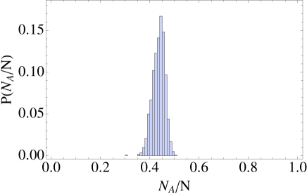
Fig. 10: Histogram of the ratio of the number of original type-$A$ cells with a large-amplitude limit cycle to the total number of cells. Here, $N=100$ cells are used with 200 sets of randomly chosen initial values for $(x_{i},y_{i})$ distributed homogeneously between 0 and 1. After the expressions reached the steady state, the ratio is computed to construct the histogram.

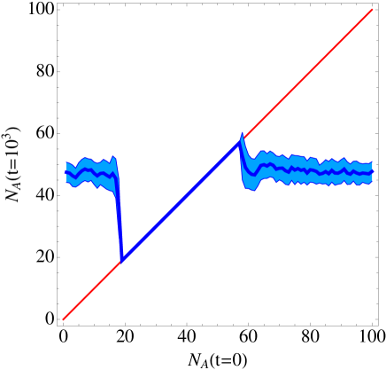
Fig. 11: The range of differentiated cell types obtained from an initial condition of two types of cells. The abscissa is the initial number of type A cells (the original cell type with a large-amplitude limit cycle) among 100 cells, and the ordinate is the number of such cells after reaching the steady state at $t=100$. For each initial number of type A cells, 200 initial conditions are chosen for the $(x_{i},y_{i})$ cells. The dark blue line shows the average of the ratio of type A cells over the 200 samples, while the blue bars show the range of the standard deviation from the distribution.

We have identified three classes of cell differentiation in terms of dynamical systems theory. The first class is that in which multiple attractors exist, where the switch among the attractors by noise leads to cell differentiation. The second is a Turing-type class in which the initial cell state is unstable and leads to two different states. The third class is asymmetric differentiation from an oscillatory state. Only the third class has a type of cell that can both proliferate and differentiate, which reflects the nature of stem cells.

In the multiple-attractor case, the differentiation is due to noise so that the time course of the development is stochastic; the number ratio of each cell type is unregulated. In the Turing-type case, the original cell type just disappears, so that there is no stem-cell-like cell.

One merit of asymmetric differentiation lies in both the existence of stem-cell-type cells and the robustness of the ratio of each cell-type number against noise Furusawa-KK01 ; SFK or a change in the initial conditions. This robustness is expected, as the differentiated cell type appears as a result of the instability of the state consisting of the first cell type only, and the two cell types stabilize each other through cell–cell interactions. In this section, we call the original cells with a large-amplitude limit cycle as type-A cells, and differentiated cells with a small-amplitude limit cycle as type-B cells and study the robustness in the number ratio of type A and B cells. To examine this robustness, we first simulated our model starting with a single cell for a given initial condition and progressively added noise. We confirmed that the ratio of one type of cell to the total number of cells has a narrow distribution even in the presence of noise, once the total number of cells reached a particular number (e.g., 32).

We then started with $N$ initial cells with random initial values of $(x_{i},y_{i})$ distributed homogeneously between 0 and 1. As shown in Fig. 10, the ratio has a narrow distribution centered around 0.43. To check the possible range of numbers of the two cell types, we simulated the model with initial conditions of the expression levels so that there were $N_{A}$ type-$A$ cells and $N-N_{A}$ differentiated cells. If $N_{A}$ is initially too large, then the state is unstable, and some of the $N_{A}$ cells show a SNIC bifurcation to lose the oscillation and differentiate to type-$B$ cells with fixed-point behavior. If $N_{A}$ is initially too small, (i.e., the proportion of differentiated cells of type $N_{B}$ is too large), then the type-$B$ state is unstable and some of these type-$B$ cells regain the oscillation to de-differentiate to type-$A$ cells. Thus, there are upper and lower bounds on the ratio of the number of type-$A$ cells. For example, in the parameter values used in Fig. 11, this range is 0.2 to 0.55. Therefore, the robustness of the two types of cells is a consequence of the present asymmetric differentiation based on the SNIC.

III.4 Complex cell differentiation by combining two-gene motifs

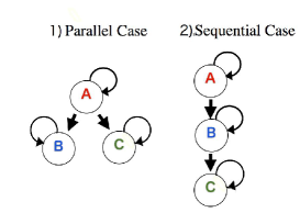
Fig. 12: Basic cell lineage diagram. Complex differentiation is composed of a combination of these two processes. (a) Parallel case: two types of cells are created from one type of cell. (b) Sequential case: cells differentiate in series.

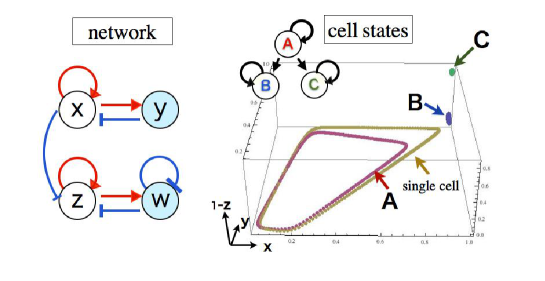
Fig. 13: The parallel case. (a) The GRN. (b) The dynamics of the three cell types are plotted as orbits in $x,y,z$ space. When asymmetric differentiation occurs in the $x$–$y$ network, the protein $z$ is expressed, which leads to a Turing instability. As a result, cells with small-amplitude oscillations in the $x$–$y$ plane split into two states with regard to the value of $z$ (type-$B$ and -$C$ cells).The parameter values that show this differentiation are$(D_{y},D_{w},g_{x},g_{y},g_{z},g_{w})=(0.2,0.2,-0.1,0.2,0.998,0)$

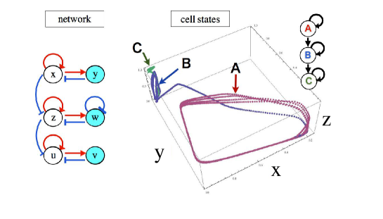
Fig. 14: The sequential case. (a) The GRN. (b) The dynamics of the three cell types are plotted as orbits in $x,y,u$ space. Asymmetric differentiation occurs in the $x$–$y$ network and some cells change from type-$A$ to type-$B$ cells. The type-$B$ cells show asymmetric differentiation in the $u$–$v$ gene network, which results in some type-$B$ cells changing into type-$C$ cells. The parameter values that show this differentiation are $(D_{y},D_{w},D_{v})$$=(0.2,0.2,0.2)$, $(g_{x}$,$g_{y}$,$g_{z}$,$g_{w}$,$g_{u}$,$g_{v}$) =(-0.1,0.2,0.99,0.0,-0.07,-0.2).$J_{m\ell}=1$ if the gene $\ell$ activates the expression of $m$, $-1$ if it inhibits the expression, and 0 if there is no regulation. But note that $J_{uz}=-0.07$.

Most of the present cells consist of a large number of cell types that are generated through successive differentiations. The entire cell lineage can be constructed by combining the following two differentiation processes.

(i) The parallel case: bifurcation into two types of cells from one type of cell, as shown in Fig. 12(a).

(ii) The sequential case: cells differentiate in series to form a hierarchical differentiation, as shown in Fig. 12(b).

Complex cell differentiations as observed in a hematopoietic system, for example, are shaped by combining these parallel and sequential differentiations. We show here that these two basic forms are designed straightforwardly by combining the Turing-type module and the asymmetric differentiation module.

The parallel case can be achieved by a gene network as shown in Fig. 13. The Turing-type module is regulated by the asymmetric differentiation module. There are four proteins $x,y,z,$ and $w$ in total whose concentrations are represented by the corresponding variables. The protein levels of the cells initially show oscillations, forming a large-amplitude limit cycle in the $x$–$y$ plane (type-$A$ cells). As the number of cells increases, asymmetric differentiation occurs in the $x$–$y$ plane to form a state with constant, higher expressions of $x$ and $y$ via the mechanism mentioned earlier. With this activation of $x$, a Turing-type bifurcation in the $z$ and $w$ protein expressions is induced. Both $z$ and $w$ are expressed in the beginning, but following the suppression of $z$, the state differentiates into two types of cells with higher and lower expressions of both $z$ and $w$ based on the Turing-type mechanism. Hence, the differentiation from stem-cell-type $A$ to two types of cells $B$ and $C$ occurs, as shown in Fig. 13.

The sequential case, however, involves the gene network shown in Fig. 14 in which two asymmetric differentiation motifs ($(x,y)$ and $(u,v)$) are connected in sequence with the intervening Turing motif ($z,w$). Here again, all the cells initially show oscillation and form a large-amplitude limit cycle in the $(x,y)$ plane (type-$A$ cells). As the number of cells increases, asymmetric differentiations occur and some cells differentiate into type-$B$ cells, which fall on a small-amplitude limit cycle in the $(x,y)$ plane. After this bifurcation, the expression of $x$ is constantly activated in the type-$B$ cells, which then suppresses the expression of $z$ and activate the expression of $u$, triggering the asymmetric differentiation of the expressions of ($u,v)$ and leading to the differentiation to type-$C$ cells with a constant activation of $u$. Thus, hierarchical, sequential differentiation from type-$A$ to $B$ and then to $C$ is generated, through which the oscillation amplitude decreases accordingly. (Here, the intermediate Turing module is used to suppress the expression level of $z$ when the expression of $x$ is constantly activated and to activate the expression otherwise. This is not an essential component, as we believe other network forms can be adopted.)

IV Discussion

We have studied in this paper an interacting cell model consisting of two genes (protein expressions) and extracted, from extensive simulation, minimal gene networks that show differentiations. These differentiations were classified as Turing, oscillation death, or asymmetric differentiation with remnant oscillations (see also Volkov ; Volkov2 for other possible types for differentiation including an inhomogeneous limit cycle in which two limit cycles coexist). Only asymmetric differentiation was shown to allow for cells with stemness, i.e., compatibility with both proliferation and differentiation. The differentiation is understood as a SNIC bifurcation which is triggered by cell–cell interactions with the cell number of the original cell type being the bifurcation parameter. It was shown that each cellular state is stabilized according to the cell–cell interaction, which depends on the number distribution of each cell type. The number ratio is thus regulated autonomously. In this sense, the effective bifurcation parameter due to cell–cell interactions is “self-consistently” determined Nakajima . A theoretical analysis for such a self-consistent bifurcation should be developed in future.

With the present study, we can now answer the questions addressed in the Introduction. (i) Which attractor describes the two conflicting functions in stem cells, i.e., proliferation and differentiation? – A single-cell attractor providing stemness is a limit-cycle that is close to the point of SNIC bifurcation. The limit-cycle attractor provides stability, while the cellular state is easily switched to a different state with the aid of SNIC bifurcation, due to cell-cell interaction. (ii) How are initial conditions for different attracting states selected through the course of development? – With the cell-cell interaction, desynchronization of oscillations follows, which diversifies the cellular states. Then, with the cell-cell interaction, states of some cells are kicked out from the original basin of attraction, triggered by SNIC bifurcation. (iii) How is the stability of the developmental course explained, which possibly includes regulation of the cell–cell interactions? – Since the desnchronization and bifurcation occur as a result of the increase in cell number, the differentiation timing is almost deterministic through the developmental course. The cell types thus generated are stabilized with each other through cell-cell interaction, which depends on the number ratio of each cell type. Hence the ratio of each cell-type is regulated so that it stays within a certain proportion, and it is robust to noise.

We were able to extract the minimal gene expression network for the stemness and demonstrated that it consists of two genes; one activates and suppresses the other, while the other has an activation path to itself. Due to the simplicity, the network can work as a motif Alon for complex cell differentiation in general. In fact, several networks previously studied for three or more genes SFK include the present minimal network motif as their core component. By including feedback or feed-forward path(s) for gene expression networks to the extracted minimal network, stem-cell-type behavior as well as the differentiation process further enhances the robustness against change in the parameter values.

Although we have adopted a simple form of the threshold expression dynamics, the bifurcation analysis developed here shows that the present mechanism for differentiation is possible in other forms of the expression dynamics, as long as the SNIC occurs due to the cell–cell interaction or signal molecule. For example, by using the Hill form for the expression,

$$\begin{split}\epsilon\frac{dx_{i}(t)}{dt}&=\frac{(\frac{x_{i}(t)}{K_{x_{1}}})^{n_{1}}}{1+(\frac{x_{i}(t)}{K_{x_{1}}})^{n_{1}}}\frac{1}{1+(\frac{y_{i}(t)}{K_{y}})^{n_{2}}}-x_{i}(t)+I_{1}\\ \frac{dy_{i}(t)}{dt}&=\frac{(\frac{x_{i}(t)}{K_{x_{2}}})^{n_{3}}}{1+(\frac{x_{i}(t)}{K_{x_{2}}})^{n_{3}}}-y_{i}(t)+I_{2}+D\Bigl{(}\sum_{k=1}^{N}y_{k}(t)-y_{i}(t)\Bigl{)},\\ \end{split}$$ (4)

the present differentiation progresses for appropriate values of the parameters (with Hill coefficients $n_{i}$ ($i=1,2,3$) of sufficiently large values).

Real GRNs, however, include more than a thousand genes, and actual networks are quite complicated. In spite of this, the present network motif, as it is so small, can be easily included in the networks of the present cell. A combination of the present two-gene network motifs can lead to differentiations of a complex cell lineage, as was demonstrated here. It will be important to extract such network motif combinations in relation to the observed complex differentiation real .

Acknowledgement:

The authors would like to thank Shuji Ishihara, Chikara Furusawa, Benjamin Pfeuty, and Narito Suzuki for useful discussions. This work was partially supported by a Grant-in-Aid for Scientific Research (No. 21120004) on Innovative Areas “Neural creativity for communication” (No. 4103) and the Platform for Dynamic Approaches to Living System from MEXT, Japan.

References

- (1) Lanza R, Gearhart J, Hogan B, Melton D, Pedersen R, Thomas ED, Thomson J, West M (2009) Essentials of Stem Cell Biology. 2nd edition, Academic Press, San Diego, USA
- (2) Potten CS, Loeffer M (1990) Development 110: 1001-1020
- (3) Ramalho-Santos M, Yoon S, Matsuzaki Y, Mulligan RC, Melton DA (2002) Science 298: 597-600
- (4) Slack JM (2002) Nat. Rev. Genet. 3: 889-895
- (5) C. H. Waddington (1957) The Strategy of the Genes. George Allen & Unwin, London
- (6) Forgacs G, Newman SA (2006) Biological Physics of The Developing Embryo. Cambridge Univ. Press, Cambridge, UK
- (7) Goodwin BC (1963) Temporal Organizations in Cells. Academic Press, San Diego, USA
- (8) Kauffman SA (1993) The Origins of Order: Self-Organization and Selection in Evolution. Oxford University Press, Oxford, UK
- (9) Kauffman SA (1969) J. Theor. Biol. 22: 437-467
- (10) Glass L, Kauffman SA (1973) J. Theor Biol. 39: 103-129
- (11) Chang HH, Hemberg M, Barahona M, Ingber DE, Huang S (2008) Nature 453: 544-548
- (12) Kaneko K, Yomo T (1994) Physica D 75: 89-102
- (13) Kaneko K, Yomo T (1997) Bull. Math. Biol. 59: 139-196
- (14) Kaneko K, Yomo T (1999) J. Theor. Biol. 199: 243-256
- (15) Furusawa C, Kaneko K (1998) Bull. Math. Biol. 60: 659-687
- (16) Furusawa C, Kaneko K (2001) J. Theor. Biol. 209: 395-416
- (17) N. Suzuki, C. Furusawa, K. Kaneko (2011), PLoS One 6, e27232.
- (18) Kobayashi T, Mizuno H, Imayoshi I, Furusawa C, Shirahige K, Kageyama R (2009) Genes Dev. 23(16): 1870-1875
- (19) Furusawa C, Kaneko K (2012) Science 338: 215-217
- (20) Mjolsness E, Sharp DH, Reinitz J (1991) J. Theor. Biol. 152: 429-453
- (21) Turing A M (1952) Phil. Trans. Roy. Soc. B 237: 37-72
- (22) Mizuguchi T, Sano M (1995) Phys. Rev. Lett. 75: 966-969
- (23) Prigogine I, Lefever R (1968) J. Chem. Phys. 48: 1695-1700
- (24) Bar-Eli K (1985) Physica D 14: 242-252; Aronson D, Ermentrout GB, Kopell N (1990) Physica D 41: 403-449
- (25) Koseska A, Volkov E, Kurths J (2010) Chaos 20: 023132
- (26) Izhikevich EM (2006) Dynamical systems in neuroscience: the geometry of excitability and bursting. MIT Press, Cambridge, MA
- (27) Ermentrout GB, Kopell N (1986) SIAM J. Appl. Math. 46: 233-253
- (28) Kaneko K (1990) Physica D 41: 137-172
- (29) Okuda K (1993) Physica D 63: 424-436
- (30) Pattern formation based on this type of oscillation dynamics is discussed in Cooke J, Zeeman EC (1976) J. Theor. Biol. 58: 455-476; Gierer A, Meinhardt H (1972) Kybernetik 12: 30-39
- (31) Nakajima A, Kaneko K (2008) J. Theor. Biol. 253: 779-787
- (32) Milo R, Shen-Orr S, Itzkovitz S, Kashtan N, Chklovskii D, Alon U (2002) Science 298: 824-827
- (33) Ullner E, Zaikin A, Volkov EI, García-Ojalvo J (2007) Phys. Rev. Lett. 99: 148103
- (34) Koseska A, Ullner E, Volkov EI, Kurths J, García-Ojalvo J, (2010), J. Theor. Biol. 263: 189-202
- (35) Morrison SJ, Shah NM, Anderson DJ (1997) Cell 88: 287-298; Loh YH, et al. (2006) Nat. Genet. 38: 431-440