Equilibrium and nonequilibrium many-body perturbation theory: a unified framework based on the Martin-Schwinger hierarchy

Abstract

We present a unified framework for equilibrium and nonequilibrium many-body perturbation theory. The most general nonequilibrium many-body theory valid for general initial states is based on a time-contour originally introduced by Konstantinov and Perel’. The various other well-known formalisms of Keldysh, Matsubara and the zero-temperature formalism are then derived as special cases that arise under different assumptions. We further present a single simple proof of Wick’s theorem that is at the same time valid in all these flavors of many-body theory. It arises simply as a solution of the equations of the Martin-Schwinger hierarchy for the noninteracting many-particle Green’s function with appropriate boundary conditions. We further discuss a generalized Wick theorem for general initial states on the Keldysh contour and derive how the formalisms based on the Keldysh and Konstantinov-Perel’-contours are related for the case of general initial states.

1 Introduction

In many physical situations we are interested in knowing the expectation value of some observable quantity of a system in or out of equilibrium. For quantum systems of many identical and interacting particles a very convenient mathematical object to extract this information is the Green’s function. Let $\hat{\rho}$ be the density matrix which describes the system at time, say, $t_{0}$ and $\hat{H}(t)$ be the Hamiltonian of the system for times $t>t_{0}$. The $n$-particle Green’s function $G_{n}$ is defined according to

$$G_{n}(1\ldots n;1^{\prime}\ldots n^{\prime})=\frac{1}{i^{n}}\Tr\left[\hat{\rho}\;T\left\{\hat{\psi}_{H}(1)\ldots\hat{\psi}_{H}(n)\hat{\psi}_{H}^{{\dagger}}(n^{\prime})\ldots\hat{\psi}_{H}(1^{\prime})\right\}\right].$$ (1)

In this formula $1=(x_{1},t_{1})$, $2=(x_{2},t_{2})$, etc. are collective indices for the position-spin coordinates $x={\bf r},\sigma$ and time $t$, the symbol $\Tr$ denotes a trace over the Fock space, $T$ is the time-ordering operator and $\hat{\psi}_{H}(j)=\hat{U}(t_{0},t_{j})\hat{\psi}(j)\hat{U}(t_{j},t_{0})$ are field operators in the Heisenberg picture with respect to the Hamiltonian $\hat{H}$ (hence $\hat{U}$ is the evolution operator). The quantum average of a $n$-body operator can be calculated from the equal-time Green’s function $G_{n}$.

The direct evaluation of $G_{n}$ from Eq. (1) is, in general, an impossible task. The first difficulty is brought by the Hamiltonian $\hat{H}=\hat{H}_{0}+\hat{H}_{\rm int}$ which is typically the sum of a one-body operator $\hat{H}_{0}$ and a $m$-body operator $\hat{H}_{\rm int}$ with $m\geq 2$. For $\hat{H}_{\rm int}\neq 0$ the field operator $\hat{\psi}_{H}$ in the Heisenberg picture is a complicated object and must be approximated in some clever way. The second difficulty consists in taking the trace over the Fock space with a density matrix $\hat{\rho}$. The density matrix is a self-adjoint, positive semi-definite operator with unit trace and, therefore, it can be written as $\hat{\rho}=e^{-\hat{X}}/\Tr[\hat{X}]$ where $\hat{X}$ is a self-adjoint operator. For instance for systems in equilibrium $\hat{X}=\beta\hat{H}^{\rm M}$ with $\beta$ the inverse temperature and $\hat{H}^{\rm M}=\hat{H}-\mu\hat{N}$ the grand-canonical Hamiltonian. To make contact with this equilibrium situation we define $\hat{H}^{\rm M}=\hat{X}/\beta$ so that

$$\hat{\rho}=\frac{e^{-\beta\hat{H}^{\rm M}}}{Z}$$ (2)

with $Z=\Tr[e^{-\beta\hat{H}^{\rm M}}]$. In equilibrium $Z$ is the partition function. In order to specify the initial preparation of the system we can assign either $\hat{\rho}$ or $\hat{H}^{\rm M}$ since there is a one-to-one correspondence between the two. If we now separate $\hat{H}^{\rm M}=\hat{H}^{\rm M}_{0}+\hat{H}^{\rm M}_{\rm int}$ into the sum of a one-body operator $\hat{H}^{\rm M}_{0}$ and a $m$-body operator $\hat{H}^{\rm M}_{\rm int}$ with $m\geq 2$ then the trace in Eq. (1) can easily be worked out for $\hat{H}^{\rm M}_{\rm int}=0$ whereas we have to use suitable approximation schemes for $\hat{H}^{\rm M}_{\rm int}\neq 0$.

Different Many-Body Perturbation Theories (MBPT) have been put forward to overcome these difficulties. The most popular MBPT’s are probably the zero-temperature (real-time) Green’s Function Formalism (GFF) and the finite-temperature (imaginary-time) Matsubara GFF [1]. These two formalisms are limited to equilibrium situations. Systems driven out of equilibrium by an external field are usually studied within the (adiabatic real-time) Keldysh GFF [2, 3]. The Keldysh GFF, however, neglects the effect of initial correlations which are relevant in the short-time dynamics of general quantum systems, such as in transient dynamics in quantum transport or in the study of atoms and molecules in external laser fields. There exist two alternative GFF’s to include initial correlations. The first is based on the idea of Konstantinov and Perel’ [4] and consists in attaching the imaginary-time Matsubara track to the original Keldysh contour, see Refs. [3, 5, 6]. The second GFF does instead account for initial correlations through extra Feynman diagrams, the evaluation of which requires the knowledge of the reduced $n$-particle density matrices

$$\Gamma_{n}(x_{1}\ldots x_{n};x^{\prime}_{1}\ldots x^{\prime}_{n})=\Tr[\hat{\rho}\,\hat{\psi}^{{\dagger}}(x^{\prime}_{1})\ldots\hat{\psi}^{{\dagger}}(x^{\prime}_{n})\hat{\psi}(x_{n})\ldots\hat{\psi}(x_{1})]$$ (3)

where the symbol $\Tr$ signifies a trace over the Fock space, see Refs. [7, 8, 9, 10, 11, 12]. These last two formalisms are both exact and hence equivalent.

In all the aforementioned GFF’s the dressed (interacting) $G_{n}$ is expanded in powers of the interaction Hamiltonian ($\hat{H}_{\rm int}$ and/or $\hat{H}_{\rm int}^{\rm M}$), leading to an expansion of $G_{n}$ in terms of the bare (noninteracting) Green’s functions $G_{0,n}$. The appealing feature of any GFF is the possibility of reducing the $G_{0,n}$ to an (anti)symmetrized product of $G_{0}\equiv G_{0,1}$ by means of Wick’s theorem [13]. Even though the mathematical structure of all GFF’s is identical, these formalisms are usually treated as independent probably due to the fact that the existing proofs of Wick’s theorem are very much formalism-dependent. In this paper we show that Wick’s theorem is the solution of a boundary problem for the Martin-Schwinger Hierarchy (MSH) [14] and that different GFF’s correspond to different domains and parameters for the MSH [15]. In this way we can easily explain the common mathematical structure of every GFF and see how, e.g., the Keldysh GFF reduces to the zero-temperature GFF in equilibrium or the Konstantinov-Perel’ GFF reduces to the Keldysh GFF under the adiabatic assumption. Our reformulation also allows us to prove a generalized Wick’s theorem for interacting density matrices $\hat{\rho}$. This naturally leads to the diagrammatic expansion with extra Feynman diagrams previously mentioned. The generalized Wick expansion has a form identical to that of a Laplace expansion for permanents/determinants (for bosons/fermions). Consequently, the calculation of the various prefactors is both explicit and greatly simplified. In this contribution we only state the generalized Wick’s theorem and refer the reader to Refs. [12, 15] for the proof. We will, however, discuss the equivalence between the GFF based on the generalized Wick’s theorem and the Konstantinov-Perel’ GFF.

2 General formula for the Green’s function

The $n$-particle Green’s function in Eq. (1) can also be written as

$$G_{n}(1\ldots n;1^{\prime}\ldots n^{\prime})=\frac{1}{i^{n}}\Tr\left[\hat{\rho}\;\mbox{$\mathcal{T}$}\left\{e^{-i\int_{\gamma}dz\hat{H}(z)}\hat{\psi}(1)\ldots\hat{\psi}(n)\hat{\psi}^{{\dagger}}(n^{\prime})\ldots\hat{\psi}(1^{\prime})\right\}\right].$$ (4)

Let us explain this formula and discuss the equivalence with Eq. (1). In Eq. (4) the integral is over the contour $\gamma$ of Fig. 1 which goes from $t_{0}$ to $\infty$ and back to $t_{0}$ whereas $\mathcal{T}$ is the contour ordering operator which rearranges operators with later contour arguments to the left. We denote by $z=t_{\pm}$ the points on $\gamma$ lying on the lower/upper branch at a distance $t$ from the origin and define the field operators with arguments on the contour as

Figure 1: Contour $\gamma$ of Eq. (4). The contour consists of a forward branch going from $t_{0}$ to $\infty$ (on this branch the points are denoted by $z=t_{-}$) and a backward branch going from $\infty$ to $t_{0}$ (on this branch the points are denoted by $z=t_{+}$).

$$\hat{\psi}(x,z)=\hat{\psi}(x).$$ (5)

More generally every operator $\hat{O}(t)$ with a real-time argument can be converted into an operator $\hat{O}(z)$ with a contour-time argument according to the rule $\hat{O}(t_{+})=\hat{O}(t_{-})=\hat{O}(t)$. In particular $\hat{H}(t_{-})=\hat{H}(t_{+})=\hat{H}(t)$. The reason to keep the contour argument in Eq. (4) even for operators that do not have an explicit time dependence (like the field operators) stems from the need of specifying their position along the contour, thus rendering unambiguous the action of $\mathcal{T}$. Once the operators are ordered we can omit the time arguments if there is no time dependence. For instance if $t_{1}<t_{2}$ then

$$\mbox{$\mathcal{T}$}\left\{e^{-i\int_{\gamma}dz\hat{H}(z)}\hat{\psi}(x_{1},t_{1-})\hat{\psi}^{{\dagger}}(x_{2},t_{2-})\right\} = \pm\hat{U}(t_{0},\infty)\hat{U}(\infty,t_{2})\hat{\psi}^{{\dagger}}(x_{2})\hat{U}(t_{2},t_{1})\hat{\psi}(x_{1})\hat{U}(t_{1},t_{0})$$ (6)

$$= T\left\{\hat{\psi}_{H}(x_{1},t_{1})\hat{\psi}^{{\dagger}}_{H}(x_{2},t_{2})\right\},$$

where the $\pm$ sign in the first equality is for bosons/fermions. One can verify that Eq. (6) is valid also for $t_{1}>t_{2}$. This example can easily be generalized to many field operators. We conclude that Eq. (4) is equivalent to Eq. (1) for contour arguments on the upper branch of $\gamma$. The $G_{n}$ in Eq. (4) is, however, more general since the contour arguments can lie either on the upper or lower branch of $\gamma$. Quantities like photoemission currents, hyper-polarizabilities and more generally high-order response properties require the knowledge of this more general Green’s function.

Figure 2: Contour $\gamma$ and Hamiltonian along the contour $\gamma$ to get the exact (Konstantinov-Perel’) Green’s function from Eq. (8).

The density matrix in Eq. (4) can be incorporated into the contour ordering operator if we extend $\gamma$ as illustrated in Fig. 2 and define the Hamiltonian with imaginary-time arguments as $\hat{H}(t_{0}-i\tau)=\hat{H}^{\rm M}$. Since

$$e^{-\beta\hat{H}^{\rm M}}=e^{-i\int_{t_{0}}^{t_{0}-i\beta}\hat{H}(z)}=\mbox{$\mathcal{T}$}\left\{e^{-i\int_{t_{0}}^{t_{0}-i\beta}\hat{H}(z)}\right\}$$ (7)

we have

$$G_{n}(1\ldots n;1^{\prime}\ldots n^{\prime})=\frac{1}{i^{n}}\frac{\Tr\left[\mbox{$\mathcal{T}$}\left\{e^{-i\int_{\gamma}dz\hat{H}(z)}\hat{\psi}(1)\ldots\hat{\psi}(n)\hat{\psi}^{{\dagger}}(n^{\prime})\ldots\hat{\psi}(1^{\prime})\right\}\right]}{\Tr\left[\mbox{$\mathcal{T}$}\left\{e^{-i\int_{\gamma}dz\hat{H}(z)}\right\}\right]}$$ (8)

where in the denominator we took into account that $\mbox{$\mathcal{T}$}\big{\{}e^{-i\int_{t_{0-}}^{t_{0+}}dz\hat{H}(z)}\big{\}}=\hat{U}(t_{0},\infty)\hat{U}(\infty,t_{0})=1$. Equation (8) is, by construction, equivalent to Eq. (4). It gives the exact Green’s function provided that the integral is done along the contour $\gamma$ of Fig. 2 and provided that the Hamiltonian changes along the contour as illustrated in the same figure. We now show that the Green’s function of every GFF can be written as in Eq. (8), the only difference being the shape of $\gamma$ and the Hamiltonian along $\gamma$.

We mentioned in the introduction that the calculation of the trace simplifies if the density matrix is of the form $\hat{\rho}_{0}=e^{-\beta\hat{H}_{0}^{\rm M}}/Z_{0}$, with $\hat{H}_{0}^{\rm M}$ a one-body operator and $Z_{0}=\Tr[e^{-\beta\hat{H}_{0}^{\rm M}}]$. It is possible to turn a trace with $\hat{\rho}$ into a trace with $\hat{\rho}_{0}$ if the adiabatic assumption is fulfilled. According to the adiabatic assumption one can generate the density matrix $\hat{\rho}$ with Hamiltonian $\hat{H}^{\rm M}=\hat{H}_{0}^{\rm M}+\hat{H}_{\rm int}^{\rm M}$ starting from the density matrix $\hat{\rho}_{0}$ with Hamiltonian $\hat{H}_{0}^{\rm M}$ and then switching on $\hat{H}^{\rm M}_{\rm int}$ adiabatically, i.e.,

$$\hat{\rho}=\frac{e^{-\beta\hat{H}^{\rm M}}}{Z}=\hat{U}_{\eta}(t_{0},-\infty)\,\frac{e^{-\beta\hat{H}_{0}^{\rm M}}}{Z_{0}}\,\hat{U}_{\eta}(-\infty,t_{0})=\hat{U}_{\eta}(t_{0},-\infty)\,\hat{\rho}_{0}\,\hat{U}_{\eta}(-\infty,t_{0}),$$ (9)

where $\hat{U}_{\eta}$ is the real-time evolution operator with Hamiltonian

$$\hat{H}_{\eta}(t)=\hat{H}_{0}^{\rm M}+e^{-\eta|t-t_{0}|}\hat{H}^{\rm M}_{\rm int},$$

and $\eta$ is an infinitesimally small positive constant. This Hamiltonian is equal to $\hat{H}_{0}^{\rm M}$ when $t\rightarrow-\infty$ and is equal to the full interacting $\hat{H}^{\rm M}$ when $t=t_{0}$. In general the validity of the adiabatic assumption should be checked case by case. Under the adiabatic assumption we can rewrite Eq. (4) as (omitting the arguments of $G_{n}$)

$$G_{n}=\frac{1}{i^{n}}\Tr\left[\hat{\rho}_{0}\;\hat{U}_{\eta}(-\infty,t_{0})\mbox{$\mathcal{T}$}\left\{e^{-i\int_{\gamma}dz\hat{H}(z)}\hat{\psi}(1)\ldots\hat{\psi}(n)\hat{\psi}^{{\dagger}}(n^{\prime})\ldots\hat{\psi}(1^{\prime})\right\}\hat{U}_{\eta}(t_{0},-\infty)\right].$$ (10)

Figure 3: Contour $\gamma$ and Hamiltonian along the contour $\gamma$ to get the adiabatic (Keldysh) Green’s function from Eq. (8).

We now see that if we construct the contour $\gamma$ of Fig. 3 and let the Hamiltonian change along the contour as

$$\hat{H}(t_{\pm})=\left\{\begin{array}[]{ll}\hat{H}_{\eta}(t)=\hat{H}_{0}^{\rm M}+e^{-\eta|t-t_{0}|}\hat{H}^{\rm M}_{\rm int}&\quad\textrm{for $t<t_{0}$}\\ \\ \;\,\hat{H}(t)=\hat{H}_{0}(t)+\hat{H}_{\rm int}(t)&\quad\textrm{for $t>t_{0}$}\end{array}\right.$$ (14)

$$\hat{H}(z\in\gamma^{\rm M})=\hat{H}_{0}^{\rm M}=\hat{H}_{0}-\mu\hat{N},$$

then Eq. (10) takes the same form as Eq. (8). We will refer to this way of calculating $G_{n}$ as the adiabatic formula. This is exactly the formula used by Keldysh in his original paper [2]. The adiabatic formula is correct only provided that the adiabatic assumption is fulfilled.

We can derive yet another expression of $G_{n}$ for systems in equilibrium at zero temperature. In equilibrium $\hat{H}^{\rm M}=\hat{H}-\mu\hat{N}$ and therefore $\hat{H}_{0}^{\rm M}=\hat{H}_{0}-\mu\hat{N}$ and $\hat{H}_{\rm int}^{\rm M}=\hat{H}_{\rm int}$. Assuming that $\hat{H}_{0}$ and $\hat{H}_{\rm int}$ commute with $\hat{N}$ the evolution operator $\hat{U}_{\eta}$ in Eq. (9) can be calculated with Hamiltonian

$$\hat{H}_{\eta}(t)=\hat{H}_{0}+e^{-\eta|t-t_{0}|}\hat{H}_{\rm int}$$ (15)

since the addition of $-\mu\hat{N}$ corresponds to multiplying $\hat{U}_{\eta}$ by a phase factor. In Eq. (9) this phase factor cancels out since $\hat{U}_{\eta}(-\infty,t_{0})=[\hat{U}_{\eta}(t_{0},-\infty)]^{{\dagger}}$. Furthermore, for any finite contour-times in $G_{n}$ we can approximate the evolution operator $\hat{U}$ in the field operators $\hat{\psi}_{H}$ with the evolution operator $U_{\eta}$ since we can always choose $\eta\ll 1/|t-t_{0}|$ and hence $\hat{H}_{\eta}\sim\hat{H}$. Thus Eq. (10) becomes

$$G_{n}=\frac{1}{i^{n}}\Tr\left[\hat{\rho}_{0}\;\mbox{$\mathcal{T}$}\left\{e^{-i\int_{\gamma}dz\hat{H}(z)}\hat{\psi}(1)\ldots\hat{\psi}(n)\hat{\psi}^{{\dagger}}(n^{\prime})\ldots\hat{\psi}(1^{\prime})\right\}\right]$$ (16)

where $\gamma$ is a contour that goes from $-\infty$ to $\infty$ and back to $-\infty$ and $\hat{H}(t_{\pm})=\hat{H}_{\eta}(t)$ is the Hamiltonian of Eq. (15). Next we observe that the interacting $\hat{\rho}$ can also be generated starting from $\hat{\rho}_{0}$ and then propagating backward in time from $\infty$ to $t_{0}$ using the same evolution operator $\hat{U}_{\eta}$ since $\hat{H}_{\eta}(t_{0}-t)=\hat{H}_{\eta}(t_{0}+t)$. In other words

$$\hat{\rho}=\hat{U}_{\eta}(t_{0},\infty)\,\hat{\rho}_{0}\,\hat{U}_{\eta}(\infty,t_{0}).$$

Comparing this equation with Eq. (9) we conclude that

$$\hat{\rho}_{0}=\hat{U}_{\eta}(-\infty,\infty)\,\hat{\rho}_{0}\,\hat{U}_{\eta}(\infty,-\infty).$$ (17)

If the ground state $|\Phi_{0}\rangle$ of $\hat{H}_{0}-\mu\hat{N}$ is nondegenerate then the zero-temperature $\hat{\rho}_{0}=|\Phi_{0}\rangle\langle\Phi_{0}|$ is a pure state and Eq. (17) implies that

$$\langle\Phi_{0}|\hat{U}_{\eta}(\infty,-\infty)=e^{i\alpha_{0}}\langle\Phi_{0}|.$$ (18)

We will refer to the adiabatic assumption in combination with equilibrium at zero temperature and with the condition of no ground-state degeneracy as the zero-temperature assumption. The zero-temperature assumption can be used to manipulate Eq. (16) a bit more. We have

$$\hat{\rho}_{0}=|\Phi_{0}\rangle\langle\Phi_{0}|=\frac{|\Phi_{0}\rangle\langle\Phi_{0}|\hat{U}_{\eta}(\infty,-\infty)}{\langle\Phi_{0}|\hat{U}_{\eta}(\infty,-\infty)|\Phi_{0}\rangle}\\ =\lim_{\beta\rightarrow\infty}\frac{e^{-\beta\hat{H}_{0}^{\rm M}}\hat{U}_{\eta}(\infty,-\infty)}{\Tr\left[e^{-\beta\hat{H}_{0}^{\rm M}}\hat{U}_{\eta}(\infty,-\infty)\right]}.$$

Figure 4: Contour $\gamma$ and Hamiltonian along the contour $\gamma$ to get the zero-temperature Green’s function from Eq. (8).

Inserting this result into Eq. (16) we find that the zero-temperature Green’s function can again be written as in Eq. (8) with the contour $\gamma$ that starts at $-\infty$, goes all the way to $\infty$ and then down to $\infty-i\beta$, see Fig. 4, and with the Hamiltonian $\hat{H}(z)$ that varies along the contour as illustrated in the same figure. It is worth noticing that the contour $\gamma$ has the special property of having only a forward branch and that for the zero-temperature assumption to make sense the Hamiltonian of the system must be time independent. There is indeed no reason to expect that by switching on and off the interaction the system goes back to the same state in the presence of external driving fields.

To summarize the exact (Konstantinov-Perel’), adiabatic (Keldysh) and zero-temperature Green’s functions have the same mathematical structure, given by Eq. (8). What changes is the contour and the Hamiltonian along the contour.

3 Wick’s theorem and Many-Body Perturbation Theory

To be concrete we specialize the discussion to interaction Hamiltonians $\hat{H}_{\rm int}$ and $\hat{H}_{\rm int}^{\rm M}$ which are two-body operators. Higher order $n$-body operators lead to more voluminous equations but do not rise conceptual complications. Thus we write

$$\hat{H}_{\rm int}(z)=\frac{1}{2}\int dx_{1}dx_{2}\;v(x_{1},x_{2};z)\hat{\psi}^{{\dagger}}(x_{1})\hat{\psi}^{{\dagger}}(x_{2})\hat{\psi}(x_{2})\hat{\psi}(x_{1}).$$ (19)

In the exact (Konstantinov-Perel’) formula the interaction $v(x_{1},x_{2};z)=v(x_{1},x_{2})$ is the interparticle interaction for $z$ on the horizontal branches whereas $v(x_{1},x_{2};z)$ depends on the initial preparation for $z$ on the vertical track. For instance in equilibrium $v(x_{1},x_{2};t_{0}-i\tau)=v(x_{1},x_{2})$. On the other hand in the adiabatic (Keldysh) and zero-temperature formula $v(x_{1},x_{2};z)=e^{-\eta|t-t_{0}|}v(x_{1},x_{2})$ for $z$ on the horizontal branches whereas $v(x_{1},x_{2};z)=0$ for $z$ on the vertical track. Let us consider Eq. (8) and write the exponential of $\hat{H}$ as the product of the exponentials of $\hat{H}_{0}$ and $\hat{H}_{\rm int}$:

$$G_{n}(1\ldots n;1^{\prime}\ldots n^{\prime})=\frac{1}{i^{n}}\frac{\Tr\left[\mbox{$\mathcal{T}$}\left\{e^{-i\int_{\gamma}dz\hat{H}_{0}(z)}e^{-i\int_{\gamma}dz\hat{H}_{\rm int}(z)}\hat{\psi}(1)\ldots\hat{\psi}(n)\hat{\psi}^{{\dagger}}(n^{\prime})\ldots\hat{\psi}(1^{\prime})\right\}\right]}{\Tr\left[\mbox{$\mathcal{T}$}\left\{e^{-i\int_{\gamma}dz\hat{H}_{0}(z)}e^{-i\int_{\gamma}dz\hat{H}_{\rm int}(z)}\right\}\right]}.$$ (20)

The expansion in powers of $\hat{H}_{\rm int}$ leads to an expansion of $G_{n}$ in terms of noninteracting Green’s functions $G_{0,n}$. The $G_{0,n}$ are obtained from Eq. (20) by setting $\hat{H}_{\rm int}(z)=0$ for all $z\in\gamma$. For instance for $n=1$ we get

$$G(a;b)=\frac{\sum\limits^{\infty}_{k=0}\frac{1}{k!}\left(\frac{i}{2}\right)^{k}\int v(1;1^{\prime})\ldots v(k;k^{\prime})G_{0,2k+1}(a,1,1^{\prime},\ldots;b,1^{+},1^{\prime+},\ldots)}{\sum\limits^{\infty}_{k=0}\frac{1}{k!}\left(\frac{i}{2}\right)^{k}\int v(1;1^{\prime})\ldots v(k;k^{\prime})G_{0,2k}(1,1^{\prime},\ldots;1^{+},1^{\prime+},\ldots)},$$ (21)

for $n=2$ we get

$$G_{2}(a,b;c,d)=\frac{\sum\limits^{\infty}_{k=0}\frac{1}{k!}\left(\frac{i}{2}\right)^{k}\int v(1;1^{\prime})\ldots v(k;k^{\prime})G_{0,2k+2}(a,b,1,1^{\prime}\ldots;c,d,1^{+},1^{\prime+},\ldots)}{\sum\limits^{\infty}_{k=0}\frac{1}{k!}\left(\frac{i}{2}\right)^{k}\int v(1;1^{\prime})\ldots v(k;k^{\prime})G_{0,2k}(1,1^{\prime},\ldots;1^{+},1^{\prime+},\ldots)},$$ (22)

etc. In these equations $a=(x_{a},t_{a})$, $b=(x_{b},t_{b})$ are collective indices like $1,\;2,\ldots$, the interaction $v(j;j^{\prime})\equiv\delta(z_{j},z^{\prime}_{j})v(x_{j},x^{\prime}_{j};z_{j})$ and the integrals are over $1,1^{\prime},\ldots,k,k^{\prime}$.

The appealing feature of any GFF is the possibility of reducing the noninteracting $G_{0,n}$ to a (anti)symmetrized product for (fermions) bosons of one-particle Green’s functions $G_{0}$. This reduction is called Wick’s theorem. The existing proofs of Wick’s theorem are rather laborious and differ depending on whether one is working with the zero-temperature or Matsubara or Keldysh Green’s functions. Below we give a simple and general proof of Wick’s theorem which applies to all cases.

We consider a one-body Hamiltonian of the form

$$\hat{H}_{0}(z)=\int dx\;\hat{\psi}^{{\dagger}}(x)h(x,z)\hat{\psi}(x).$$ (23)

The more general case of a nondiagonal $h(x,x^{\prime},z)$ can be treated in a similar manner. The Green’s functions $G_{0,n}$ satisfy the noninteracting MSH

$$\left[i\frac{d}{dz_{k}}-h(k)\right]G_{0,n}(1\ldots n;1^{\prime}\ldots n^{\prime})=\sum_{j=1}^{n}\,(\pm)^{k+j}\,\delta(k;j^{\prime})\,G_{0,n-1}(1\ldots\stackrel{{\scriptstyle\sqcap}}{{k}}\ldots n;1^{\prime}\ldots\stackrel{{\scriptstyle\sqcap}}{{j^{\prime}}}\ldots n^{\prime})$$ (24)

$$G_{0,n}(1\ldots n;1^{\prime}\ldots n^{\prime})\left[-i\frac{\overleftarrow{d}}{dz_{k}^{\prime}}-h(k^{\prime})\right]=\sum_{j=1}^{n}\,(\pm)^{k+j}\,\delta(j;k^{\prime})\,G_{0,n-1}(1\ldots\stackrel{{\scriptstyle\sqcap}}{{j}}\ldots n;1^{\prime}\ldots\stackrel{{\scriptstyle\sqcap}}{{k^{\prime}}}\ldots n^{\prime})$$ (25)

where the hook over the arguments in $G_{0,n-1}$ means that those variables are missing. The MSH is a set of coupled differential equations to be solved on the contour $\gamma$ of the Green’s function of interest (exact, adiabatic, or zero-temperature). In all cases from the definition Eq. (8) it follows that the $G_{0,n}$ satisfy the Kubo-Martin-Schwinger (KMS) relations, i.e., the $G_{0,n}$ are (anti)periodic along the contour $\gamma$ with respect to all their contour arguments. Therefore we can calculate the $G_{0,n}$ by solving the MSH with KMS relations. We now show that the solution is given by the Wick theorem

$$G_{0,n}(1,\ldots,n;1^{\prime},\ldots,n^{\prime})=\left|\begin{array}[]{ccc}G_{0}(1;1^{\prime})&\ldots&G_{0}(1;n^{\prime})\\ \vdots&&\vdots\\ G_{0}(n;1^{\prime})&\ldots&G_{0}(n;n^{\prime})\end{array}\right|_{\pm}$$ (29)

where the symbol $|\ldots|_{\pm}$ signifies the permanent/determinant for the case of bosons/fermions and $G_{0}$ is the solution of Eqs. (24) and (25) with $n=1$, i.e.,

$$\left[i\frac{d}{dz_{1}}-h(1)\right]G_{0}(1;1^{\prime})=\delta(1;1^{\prime}),\quad\quad G_{0}(1;1^{\prime})\left[-i\frac{\overleftarrow{d}}{dz_{1}^{\prime}}-h(1^{\prime})\right]=\delta(1;1^{\prime})$$ (30)

with KMS boundary conditions. Expanding the permanent/determinant along row, say, $k$ we get

$$G_{0,n}(1,\ldots,n;1^{\prime},\ldots,n^{\prime})=\sum_{j=1}^{n}(\pm)^{k+j}G_{0}(k,j^{\prime})G_{0,n-1}(1\ldots\stackrel{{\scriptstyle\sqcap}}{{k}}\ldots n;1^{\prime}\ldots\stackrel{{\scriptstyle\sqcap}}{{j^{\prime}}}\ldots n^{\prime})$$ (31)

which is clearly a solution of Eq. (24). Similarly, we can readily verify that Eq. (29) is also solution of Eq. (25) by expanding the permanent/determinant along column $k$. It remains to check that the $G_{0,n}$ in Eq. (29) fulfills the KMS relations. The contour argument $z_{k}$ appears in all the $G_{0}$ of the $k$-th row of Eq. (29) and nowhere else. Therefore when we move $z_{k}$ from the starting to the ending point of $\gamma$ all entries of row $k$ pick up a $(\pm)$ sign. Since the permanent/determinant of a matrix in which we multiply a row by $(\pm)$ is $(\pm)$ the permanent/determinant of the original matrix we conclude that $G_{0,n}$ is (anti)periodic with respect to the first $n$ contour arguments. With a similar reasoning one can prove that $G_{0,n}$ is (anti)periodic with respect to the last $n$ contour arguments. This concludes the proof.

The Wick theorem has been proven without any assumption on the shape of the contour and without any assumption on the form of the single-particle Hamiltonian $h(x,z)$ along the contour. Inserting Eq. (29) into, e.g., Eq. (21) we get the MBPT formula for the one-particle Green’s function

$$G(a;b)=\frac{\sum\limits^{\infty}_{k=0}\frac{1}{k!}\left(\frac{i}{2}\right)^{k}\!\int\!v(1;1^{\prime})\,..\,v(k;k^{\prime})\!\left|\!\!\!\begin{array}[]{cccc}G_{0}(a;b)&G_{0}(a;1^{+})&\ldots&G_{0}(a;k^{\prime+})\\ G_{0}(1;b)&G_{0}(1;1^{+})&\ldots&G_{0}(1;k^{\prime+})\\ \vdots&\vdots&\ddots&\vdots\\ G_{0}(k^{\prime};b)&G_{0}(k^{\prime};1^{+})&\ldots&G_{0}(k^{\prime};k^{\prime+})\end{array}\!\!\!\right|_{\pm}}{\sum\limits^{\infty}_{k=0}\frac{1}{k!}\left(\frac{i}{2}\right)^{k}\!\int\!v(1;1^{\prime})\,..\,v(k;k^{\prime})\!\left|\!\!\!\begin{array}[]{cccc}G_{0}(1;1^{+})&G_{0}(1;1^{\prime+})&\ldots&G_{0}(1;k^{\prime+})\\ G_{0}(1^{\prime};1^{+})&G_{0}(1^{\prime};1^{\prime+})&\ldots&G_{0}(1^{\prime};k^{\prime+})\\ \vdots&\vdots&\ddots&\vdots\\ G_{0}(k^{\prime};1^{+})&G_{0}(k^{\prime};1^{\prime+})&\ldots&G_{0}(k^{\prime};k^{\prime+})\end{array}\!\!\!\right|_{\pm}\!\!}$$ (32)

which is an exact expansion of the interacting $G$ in terms of the noninteracting $G_{0}$. The MBPT for higher order Green’s functions can be derived similarly. In the next Section we discuss how the variuos GFF’s follow from Eq. (32).

4 Matsubara, Keldysh and zero-temperature formalisms

In the Konstantinov-Perel’ formalism the Green’s function $G$ is given by Eq. (32) where the $z$-integrals run on the contour of Fig. 2. It is worth stressing that if the times $t_{a}$ and $t_{b}$ in $G(a;b)$ are smaller than a maximum time $T$ then it is sufficient to perform the $z$ integrals over a shrunken contour like the one illustrated in Fig. 5. This is a direct consequence of the fact that if the contour is longer than $T$ then the terms with integrals after $T$ cancel off [15].

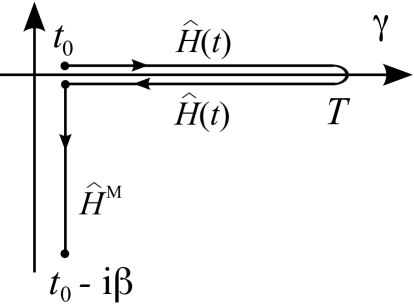
Figure 5: The shrunken contour $\gamma$ that can be used in Eq. (32) to obtain the Green’s function with real-time smaller than $T$.

The Matsubara GFF is used to calculate Green’s function with imaginary times and it is typically applied to systems in equilibrium at finite temperature. For this reason the Matsubara GFF is also called the “finite-temperature formalism”. To calculate $G$ with imaginary-time arguments we can choose $T=t_{0}$ in Fig. 5 and hence shrink the horizontal branches to a point leaving only the vertical track. Therefore the Matsubara GFF consists of expanding the Green’s function as in Eq. (32) with the $z$-integrals restricted to the vertical track. It is important to realize that no assumptions, like the adiabatic or the zero-temperature assumption, are made in this formalism. The Matsubara GFF is exact but limited to initial (or equilibrium) averages. Equivalently we can say that the Matsubara $G$ is the same as the Konstantinov-Perel’ $G$ on the vertical track.

The formalism originally used by Keldysh was based on the adiabatic assumption. The Keldysh Green’s functions are again given by Eq. (32) but the $z$-integrals are done over the contour of Fig. 3 and the Hamiltonian changes along the contour as illustrated in the same figure. The important simplification of the Keldysh GFF is that the interaction $v$ is zero on the vertical track. Consequently in Eq. (32) we can restrict the $z$-integrals to the horizontal branches. Like the Konstantinov-Perel’ formalism, the Keldysh GFF can be used to deal with nonequilibrium situations in which the external perturbing fields are switched on after time $t_{0}$. In the special case of no external fields we can calculate interacting equilibrium Green’s functions at any finite temperature with real-time arguments.

The zero-temperature formalism relies on the zero-temperature assumption. As we already discussed this assumption makes sense only in the absence of external fields. The corresponding zero-temperature Green’s function is given by Eq. (32) in which the $z$-integrals are done over the contour of Fig. 4 and the Hamiltonian changes along the contour as illustrated in the same figure. Like in the Keldysh GFF the interaction $v$ vanishes along the vertical track and hence the $z$-integrals can be restricted to a contour that goes from $-\infty$ to $\infty$. The contour ordering operator is then the same as the standard time-ordering operator. For this reason the zero-temperature Green’s function is also called time-ordered Green’s function. The zero-temperature GFF allows us to calculate the interacting $G$ in equilibrium at zero temperature with real-time arguments. It cannot, however, be used to study systems out of equilibrium and/or at finite temperature. In some cases, however, the zero-temperature formalism is used also at finite temperatures (finite $\beta$) as the finite temperature corrections are small. This approximated formalism is sometimes referred to as the real-time finite temperature formalism [1]. We emphasize that in the real-time finite-temperature formalism (like in the Keldysh formalism) the temperature enters in Eq. (32) only through $G_{0}$ which satisfies the KMS relations. In the Konstantinov-Perel’ formalism, on the other hand, the temperature enters through $G_{0}$ and through the contour integrals since the interaction is nonvanishing along the vertical track.

5 Generalized Wick’s theorem

The MBPT of the exact GFF requires the knowledge of the operator $\hat{H}^{\rm M}$ on the vertical track. In many physical situations, however, it is easier to specify the initial state (or initial density matrix) instead of $\hat{H}^{\rm M}$. In these cases the preliminary step to apply MBPT consists in obtaining $\hat{H}^{\rm M}$ from $\hat{\rho}$, something that can be rather awkward. For instance if $\hat{\rho}=|\Psi\rangle\langle\Psi|$ is a pure state then $\hat{H}^{\rm M}$ is an operator with $|\Psi\rangle$ as the ground state. The existence of a generalized Wick’s theorem that uses directly $\hat{\rho}$ would be of very valuable. In this Section we will show how to construct such a generalized framework.

We consider again Eq. (4) but this time we do not incorporate $\hat{\rho}$ in the contour ordering. In Eq. (4) the contour $\gamma$ is that of Fig. 1 and the Hamiltonian is the physical Hamiltonian which, for simplicity, we take as the sum of $\hat{H}_{0}$ in Eq. (23) and $\hat{H}_{\rm int}$ in Eq. (19). We write the exponential in Eq. (4) as the product of two exponentials, one containing $\hat{H}_{0}$ and the other containing $\hat{H}_{\rm int}$, like we did in Eq. (20). The subsequent expansion of $G$ in powers of $\hat{H}_{\rm int}$ leads to the expansion

$$G(a;b)=\sum\limits^{\infty}_{k=0}\frac{1}{k!}\left(\frac{i}{2}\right)^{k}\int v(1;1^{\prime})\ldots v(k;k^{\prime})g_{2k+1}(a,1,1^{\prime},\ldots;b,1^{+},1^{\prime+},\ldots)$$ (33)

and similarly for higher order Green’s function. In Eq. (33) the Green’s functions $g_{n}$ are noninteracting Green’s functions averaged with an arbitrary density matrix $\hat{\rho}$

$$g_{n}(1\ldots n;1^{\prime}\ldots n^{\prime})=\frac{1}{i^{n}}\Tr\left[\hat{\rho}\;\mbox{$\mathcal{T}$}\left\{e^{-i\int_{\gamma}dz\hat{H}_{0}(z)}\hat{\psi}(1)\ldots\hat{\psi}(n)\hat{\psi}^{{\dagger}}(n^{\prime})\ldots\hat{\psi}(1^{\prime})\right\}\right].$$ (34)

We will now prove a generalized Wick theorem to write these $g_{n}$ in terms of the one-particle Green’s function $g\equiv g_{1}$ and the $n$-particle reduced density matrices $\Gamma_{n}$ defined in Eq. (3).

The Green’s functions $g_{n}$ satisfy the noninteracting MSH on the contour of Fig. 1. The problem in solving the MSH to obtain the $g_{n}$’s is that we cannot use the KMS relations as boundary conditions. Indeed it is easy to verify that the $g_{n}$ are not (anti)periodic along the contour. A convenient choice of boundary conditions follows directly from the definition of $g_{n}$ and reads

$$(\pm i)^{n}\lim_{z_{k},z^{\prime}_{j}\rightarrow t_{0-}}g_{n}(1\ldots n;1^{\prime},\ldots n^{\prime})=\Gamma_{n}(x_{1}\ldots x_{n};x^{\prime}_{1}\ldots x^{\prime}_{n})$$ (35)

where the limit is taken with the order $z_{1}<\ldots<z_{n}<z^{\prime}_{n}<\ldots<z^{\prime}_{1}$ of the contour arguments. The permanent/determinant

$$g_{n}(1\ldots n;1^{\prime}\ldots n^{\prime})=\left|\begin{array}[]{ccc}g(1;1^{\prime})&&g(1;n^{\prime})\\ \vdots&\vdots&\vdots\\ g(n;1^{\prime})&&g(n;n^{\prime})\end{array}\right|_{\pm}\equiv|g|_{n}(1\ldots n;1^{\prime}\ldots n^{\prime})$$ (36)

is a solution of the MSH but, in general, with the wrong boundary conditions. In Eq. (36) the symbol $|\ldots|_{\pm}$ signifies the permanent/determinant of the matrix inside the vertical bars. The particular solution must be supplied with the solution of the homogeneous equations

$$\left[i\frac{d}{dz_{k}}-h(k)\right]\tilde{g}_{n}(1\ldots n;1^{\prime}\ldots n^{\prime})=0$$ (37)

$$\tilde{g}_{n}(1\ldots n;1^{\prime}\ldots n^{\prime})\left[-i\frac{\overleftarrow{d}}{dz_{k}^{\prime}}-h(k^{\prime})\right]=0$$ (38)

to satisfy the correct boundary conditions. We observe that $\tilde{g}_{n}$ is not discontinuous when its contour arguments cross each other since in the right hand side of Eqs. (37) and (38) there is no $\delta$-function. Consequently the equal-time limit of $\tilde{g}_{n}$ is independent of the order of the contour arguments.

Let us start by showing how to solve the MSH for $g_{2}$. We write $g_{2}=|g|_{2}+\tilde{g}_{2}$ where $g$ satisfies the first equation of the MSH with boundary conditions

$$(\pm i)\lim_{z_{1},z^{\prime}_{1}\rightarrow t_{0-}}g(1;1^{\prime})=\Gamma_{1}(x_{1};x^{\prime}_{1})\equiv\Gamma(x_{1};x^{\prime}_{1}).$$ (39)

The boundary conditions for $\tilde{g}_{2}$ follow directly from Eq. (35) and read

$$(\pm i)^{2}\lim_{z_{k},z^{\prime}_{j}\to t_{0-}}\tilde{g}_{2}=(\pm i)^{2}\lim_{z_{k},z^{\prime}_{j}\to t_{0-}}(g_{2}-|g|_{2})=\Gamma_{2}-|\Gamma|_{2}\equiv C_{2}.$$ (40)

Next we consider the spectral function on the contour

$$A(1;1^{\prime})=i\left[g^{>}(1;1^{\prime})-g^{<}(1;1^{\prime})\right].$$ (41)

This function takes the same value for $z_{1}=t_{1\pm}$ and $z^{\prime}_{1}=t^{\prime}_{1\pm}$ and satisfies the equations

$$\left[i\frac{d}{dz_{1}}-h(1)\right]A(1;1^{\prime})=A(1;1^{\prime})\left[-i\frac{\overleftarrow{d}}{dz^{\prime}_{1}}-h(1^{\prime})\right]=0.$$ (42)

Furthermore, due to the (anti)commutation rules of the field operators

$$A(x_{1},z;x^{\prime}_{1},z)=\delta(x_{1}-x^{\prime}_{1}).$$ (43)

Therefore

$$\tilde{g}_{2}(1,2;1^{\prime},2^{\prime}) = \int d\bar{x}_{1}d\bar{x}_{2}d\bar{x}^{\prime}_{1}d\bar{x}^{\prime}_{2}A(1;\bar{x}_{1},t_{0-})A(2;\bar{x}_{2},t_{0-})C_{2}(\bar{x}_{1},\bar{x}_{2};\bar{x}^{\prime}_{1},\bar{x}^{\prime}_{2})$$ (44)

$$\times A(\bar{x}^{\prime}_{1},t_{0-};1^{\prime})A(\bar{x}^{\prime}_{2},t_{0-};2^{\prime})$$

is clearly the solution of the homogeneous MSH with the correct boundary conditions, see Eq. (40). We can manipulate Eq. (44) by introducing a linear combination of $\delta$-functions on the contour

$$\delta_{-}(z)\equiv\delta(z,t_{0-})-\delta(z,t_{0+}).$$ (45)

The spectral function appearing in Eq. (44) can be written as

$$A(1;x^{\prime}_{1},t_{0-})=i\int_{\gamma}d\bar{z}\;g(1;x^{\prime}_{1},\bar{z})\delta_{-}(\bar{z})$$ (46)

and

$$A(x_{1},t_{0-};1^{\prime})=-i\int_{\gamma}d\bar{z}\;\delta_{-}(\bar{z})g(x_{1},\bar{z};1^{\prime}).$$ (47)

Inserting these expressions into Eq. (44) we find

$$\tilde{g}_{2}(1,2;1^{\prime},2^{\prime})=\int d\bar{1}d\bar{2}d\bar{1}^{\prime}d\bar{2}^{\prime}g(1;\bar{1})g(2;\bar{2})C_{2}(\bar{1},\bar{2};\bar{1}^{\prime},\bar{2}^{\prime})g(\bar{1}^{\prime};1^{\prime})g(\bar{2}^{\prime};2^{\prime})$$ (48)

where

$$C_{2}(\bar{1},\bar{2};\bar{1}^{\prime},\bar{2}^{\prime})=\delta_{-}(\bar{z}_{1})\delta_{-}(\bar{z}_{2})C_{2}(\bar{x}_{1},\bar{x}_{2};\bar{x}^{\prime}_{1},\bar{x}^{\prime}_{2})\delta_{-}(\bar{z}^{\prime}_{1})\delta_{-}(\bar{z}^{\prime}_{2})$$ (49)

is the two-particle initial-correlation function. In conclusion $\tilde{g}_{2}$ can be written in terms of $g$ and $\Gamma_{n}$ with $n\leq 2$. Since $g_{2}=|g|_{2}+\tilde{g}_{2}$ this result provides a decomposition of $g_{2}$ in terms of $g$ and reduced $n$-particle denity matrices.

The generalization of Wick’s theorem to $g_{n}$ reads

$$g_{n}=|g|_{n}+\;\sum_{l=1}^{n-2}\sum_{PQ}(\pm)^{|P+Q|}\;|g|_{l}(P;Q^{\prime})\;\tilde{g}_{n-l}(\breve{P};\breve{Q}^{\prime})\;+\;\tilde{g}_{n}.$$ (50)

In this formula $P$ and $Q$ are a subset of $l$ ordered indices between $1$ and $n$ whereas $\breve{P}$ and $\breve{Q}$ is the ordered complementary subset. For instance if $n=3$ and $l=1$ then we can have $P=1$ and hence $\breve{P}=(2,3)$, or $P=2$ and hence $\breve{P}=(1,3)$, or $P=3$ and hence $\breve{P}=(1,2)$. The sign of the various terms is given by $|P+Q|=\sum_{i=1}^{l}(p_{i}+q_{i})$ where $p_{i}$ and $q_{i}$ are the indices in the $l$-tuple $P$ and $Q$. The solution of the homogeneous MSH with the correct boundary conditions is

$$\tilde{g}_{n}(1\ldots n;1^{\prime}\ldots n^{\prime})=\int g(1;\bar{1})\ldots g(n;\bar{n})C_{n}(1\ldots n;1^{\prime}\ldots n^{\prime})g(\bar{n}^{\prime};n^{\prime})\ldots g(\bar{1}^{\prime};1^{\prime})$$ (51)

where the integral is over all barred variables and the $n$-particle initial-correlation functions are given by

$$C_{n}(1\ldots n;1^{\prime}\ldots n^{\prime})=\delta_{-}(z_{1})\ldots\delta_{-}(z_{n})C_{n}(x_{1}\ldots x_{n};x^{\prime}_{1}\ldots x^{\prime}_{n})\delta_{-}(z^{\prime}_{1})\ldots\delta_{-}(z^{\prime}_{n})$$ (52)

with

$$C_{n}=\Gamma_{n}-\sum_{l=1}^{n-2}\sum_{PQ}(\pm)^{|P+Q|}|\Gamma|_{l}(X_{P};X^{\prime}_{Q})C_{n-l}(X_{\breve{P}};X_{\breve{Q}}^{\prime})-|\Gamma|_{n}.$$ (53)

This is a recursive formula for the $C_{n}$. The collective coordinate $X_{P}=(x_{p_{1}}\ldots x_{p_{l}})$ is a subset of the coordinates $(x_{1}\ldots x_{n})$ and similarly the collective coordinate $X^{\prime}_{Q}=(x^{\prime}_{q_{1}}\ldots x^{\prime}_{q_{l}})$ is a subset of the coordinates $(x^{\prime}_{1}\ldots x^{\prime}_{n})$.

We defer the reader to Ref. [12] for the proof of the generalized Wick theorem. Here we observe that with the generalized Wick theorem we can express $g_{n}$ in terms of $g$ and $\Gamma_{n}$. Since $\Gamma_{n}$ can easily be calculated from $\hat{\rho}$ the generalized Wick theorem is especially suited to do MBPT when we know $\hat{\rho}$ instead of $\hat{H}^{\rm M}$. We further observe that the generalized Wick theorem has the same mathematical structure of the Laplace expansion for the permanent/determinant of the sum of two matrices $A$ and $B$ [15]

$$|A+B|_{m}=|A|_{m}+\sum_{l=1}^{m-1}\sum_{PQ}(\pm)^{|P+Q|}|A|_{l}(P;Q)|B|_{m-l}(\breve{P};\breve{Q})+|B|_{m}$$ (54)

where $|A|_{l}(P;Q)$ is the permanent/determinant of the $l\times l$ matrix obtained with the rows $P$ and the columns $Q$ of the matrix $A$. The same notation has been used for the matrix $B$. With the identification $A_{kj}=g(k;j^{\prime})$ and $|B|_{m-l}(\breve{P};\breve{Q})=\tilde{g}_{m-l}(\breve{P};\breve{Q}^{\prime})$ for $l=1\ldots m-2$ and the definition $\tilde{g}_{1}\equiv 0$ Eqs. (50) and (54) become identical. We can thus symbolically write the generalized Wick theorem as

$$g_{m}=|g+\tilde{g}|_{m}$$ (55)

whose precise meaning is given by Eq. (50).

6 Relation with the Konstantinov-Perel’ formalism

In Eq.(33) we have seen how we can expand the Green’s function $G$ into noninteracting Green’s functions $g_{n}$ satisfying the generalized Wick theorem (50). This can be used to define a diagrammatic expansion of the Green’s function. Let us see what terms we get when we insert Eq.(50) into Eq.(33). The first term $|g|_{n}$ in Eq.(50) generates the usual series of connected diagrams for the Green’s function in powers of the interaction (the disconnected diagrams are zero since they are integrated from $t_{0}$ to $t_{0}$ and have no external points). The remaining terms in Eq.(50) are linear in the functions $\tilde{g}_{m}$ with $m=2,\ldots,n$. As a consequence of Eq.(51) these functions can be diagrammatically represented by blocks $C_{m}$ with $m$ ingoing and $m$ outgoing $g$ lines. Since the Wick expression (50) is linear in the $\tilde{g}_{m}$ each diagram contribution to the Green’s function contains at most one correlation block. In Fig. 6 we display the diagrams for the Green’s function up to first order in the interaction involving four diagrams with a $C_{2}$ block and one diagram with a $C_{3}$ block. The last three diagrams, however, vanish since for those diagrams there are internal time-integrations for Green’s funtion lines that enter and leave a $C_{m}$ block that can be reduced to a point, since the initial correlation block only exists at time $t_{0-}$.

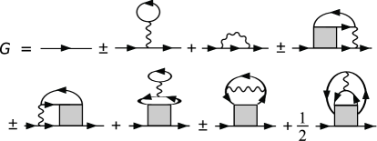
Figure 6: Diagrammatic expansion of the Green’s function to first order in the interaction.

The fact that the $C_{m}$ blocks are not repeated within a single diagram prevents us from deriving an irreducible self-energy in terms of them. We can, however, define a reducible self-energy $\sigma_{r}$ and write the Green’s function as

$$G(1;2)=g(1;2)+\int_{\bar{\gamma}}d\bar{1}d\bar{2}\,g(1;\bar{1})\sigma_{r}(\bar{1};\bar{2})g(\bar{2};2)$$ (56)

where we used the notation $\bar{\gamma}$ for the contour of Fig.1 to distinguish it from the extended contour $\gamma$ that we will use later. The reducible self-energy can be split into three contributions. These are the sets of self-energy diagrams that start with an interaction line at their entrance vertices, and end with a correlation block at their exit vertices, denoted by $\sigma_{r}^{L}$, the diagrams that start with a correlation block and end with an interaction line, denoted by $\sigma_{r}^{R}$, and the remaining diagrams (which either contain no correlation block or contain a correlation block only attached to internal vertices) which we will denoted by $\tilde{\sigma}_{r}$. The labels $L$ and $R$ therefore refer to the location of an interaction line at the entrance vertices. We can thus write

$$\sigma_{r}=\tilde{\sigma}_{r}+\sigma_{r}^{L}+\sigma_{r}^{R}$$ (57)

where

$$\sigma_{r}^{L}(1;2) = \sigma_{r}^{L}(1;x_{2})\delta_{-}(z_{2})$$ (58)

$$\sigma_{r}^{R}(1;2) = \delta_{-}(z_{1})\sigma_{r}^{R}(x_{1};2).$$ (59)

We emphasize that $\sigma_{r}$ is a reducible self-energy and therefore it should not be confused with the self-energy of Ref. [7]. We will now proceed to connect the reducible self-energy $\sigma_{r}$ to the irreducible self-energy appearing in the equation of motion for the Green’s function on the extended contour. As discussed in the introduction the initial ensemble is of the form $\hat{\rho}=e^{-\hat{X}}/\mathrm{Tr}[e^{-\hat{X}}]$, where $\hat{X}=\sum_{m}\hat{X}_{m}$ is in general a sum of $m$-body operators of the form

$$\hat{X}_{m}=\frac{1}{m!}\int dx_{1}\ldots dx_{m}^{\prime}\,v_{m}(x_{1},\ldots,x_{m},x_{1}^{\prime},\ldots,x_{m}^{\prime})\hat{\psi}^{\dagger}(x_{1})\ldots\hat{\psi}^{\dagger}(x_{m})\hat{\psi}(x_{m}^{\prime})\ldots\hat{\psi}(x_{1}^{\prime})$$ (60)

The functions $v_{m}$ must be chosen in such a way that the pre-scribed density matrices of Eq.(3) are obtained. This is, in general, a difficult task. If we, however, assume that we have succeeded in this task we can define the Matsubara Hamiltonian $\hat{H}^{\rm{M}}=\hat{X}/\beta$ and use the contour of Fig. (2) and the expression for the Green’s function (8) to expand the Green’s function diagrammatically in powers of $G_{0}$ using the standard Wick theorem of Eq.(29) [3, 5, 6]. The diagrammatic rules for the Green’s function in the case of $m$-body operators are given in Ref. [5]. If we collect the irreducible pieces of this expansion in an irreducible self-energy $\Sigma$ then we obtain a Dyson equation on the extended contour

$$G(1;2)=G_{0}(1;2)+\int_{\gamma}d3d4\,G_{0}(1;3)\Sigma(3;4)G(4,2).$$ (61)

It will be more convenient to write this as equations of motion

$$(i\partial_{z_{1}}-h(1))G(1;2) = \delta(1;2)+\int_{\gamma}d3\,\Sigma(1;3)G(3;2)$$ (62)

$$G(1;2)(-i\overleftarrow{\partial_{z_{2}}}-h(2)) = \delta(1;2)+\int_{\gamma}d3\,G(1;3)\Sigma(3;2)$$ (63)

When split into various components these are simply the Kadanoff-Baym equations on the extended contour. Let us now write the contour $\gamma$ as $\gamma=\bar{\gamma}\oplus\gamma^{\rm{M}}$, where $\gamma^{\rm{M}}$ denotes the vertical (or Matsubara) track of the contour and $\bar{\gamma}$ the remaining piece, which is identical to the contour of Fig. 1. The last term on the r.h.s of Eq.(62) can then be written as

$$\int_{\gamma}d3\,\Sigma(1;3)G(3;2)=\int_{\bar{\gamma}}d3\,\Sigma(1;3)G(3;2)-i\int dx_{3}\int_{0}^{\beta}d\tau\,\Sigma^{\rceil}(1;x_{3}\tau)G^{\lceil}(x_{3}\tau;2)$$ (64)

where we introduced the parametrization $z=t_{0}-i\tau$ on the vertical track $\gamma^{\rm{M}}$. For a general function $A(z,z^{\prime})$ on the contour (spatial coordinates suppressed) we further defined

$$A^{\rceil}(z=t_{\pm},\tau) = A(z=t_{\pm},t_{0}-i\tau)$$ (65)

$$A^{\lceil}(\tau,z=t_{\pm}) = A(t_{0}-i\tau,z=t_{\pm}).$$ (66)

From the Dyson equation (61) and the Langreth rules on the contour $\gamma$ we can further derive that [15, 16]

$$G^{\lceil}(1;2)=-i\int d\bar{x}\,G^{\rm{M}}(1;\bar{x}t_{0})G^{\rm{A}}(\bar{x}t_{0};2)+[G^{\rm{M}}\star\Sigma^{\lceil}\cdot G^{\rm{A}}](1;2)$$ (67)

where $\star$ denotes a convolution between $t_{0}$ and $t_{0}-i\beta$ on the vertical track and $\cdot$ denotes a convolution between $t_{0}$ and $\infty$. We further defined the advanced and Matsubara Green’s functions as

$$G^{\rm{A}}(1;2) = -\theta(t_{2}-t_{1})[G^{>}(1;2)-G^{<}(1;2)]$$ (68)

$$G^{\rm{M}}(1;2) = G(x_{1}t_{0}-i\tau_{1};x_{2}t_{0}-i\tau_{2})$$ (69)

If we further use that

$$\int_{\bar{\gamma}}dz\,\delta_{-}(z)G(\bar{x}z;xt_{\pm})=G^{\rm{A}}(\bar{x}t_{0};xt)$$ (70)

we find by inserting Eq.(67) into the last term of Eq.(64) that

$$-i\int dx_{3}\int_{0}^{\beta}d\tau\,\Sigma^{\rceil}(1;x_{3}\tau)G^{\lceil}(x_{3}\tau;2)=$$ (71)

$$\int_{\bar{\gamma}}d3\,[\Sigma^{\rceil}\star G^{\rm{M}}\star\Sigma^{\lceil}](1;3)G(3;2)-i\int_{\bar{\gamma}}d3\,[\Sigma^{\rceil}\star G^{\rm{M}}](1;x_{3}t_{0})\delta_{-}(z_{3})G(3;2)$$

If we therefore define $\Sigma_{\rm{L}}$ by

$$\Sigma_{\rm{L}}(1;2)=-i[\Sigma^{\rceil}\star G^{\rm{M}}](1;x_{2}t_{0})\delta_{-}(z_{2}),$$ (72)

we can rewrite the equation of motion (62) for the Green’s function as

$$(i\partial_{z_{1}}-h(1))G(1;2)=\delta(1;2)+\int_{\bar{\gamma}}d3\,[\Sigma+\Sigma^{\rceil}\star G^{\rm{M}}\star\Sigma^{\lceil}+\Sigma_{\rm{L}}](1;3)G(3;2).$$ (73)

A similar procedure can be carried out for the adjoint equation (63). We find

$$G(1;2)(-i\overleftarrow{\partial_{z_{2}}}-h(2)) = \delta(1;2)+\int_{\bar{\gamma}}d3\,G(1;3)[\Sigma+\Sigma^{\rceil}\star G^{\rm{M}}\star\Sigma^{\lceil}+\Sigma_{\rm{R}}](3;2)$$ (74)

where we defined

$$\Sigma_{\rm{R}}(1;2)=-i\delta_{-}(z_{1})[G^{\rm{M}}\star\Sigma^{\lceil}](x_{1}t_{0};2).$$ (75)

Given the self-energy and the Green’s function with arguments on the imaginary track $\gamma^{\rm{M}}$, we can regard Eqs. (73) and (74) as equations of motion for the Green’s function $G$ on the contour $\bar{\gamma}$. These equations can be integrated using the noninteracting Green’s function $g$ of Eq.(39) since it satisfies

$$(\pm i)\lim_{z_{1},z^{\prime}_{1}\rightarrow t_{0-}}g(1;1^{\prime})=(\pm i)\lim_{z_{1},z^{\prime}_{1}\rightarrow t_{0-}}G(1;1^{\prime})=\Gamma(x_{1};x^{\prime}_{1}).$$ (76)

If we, therefore, define the total self-energy as

$$\Sigma_{\rm{tot}}=\Sigma+\Sigma^{\rceil}\star G^{\rm{M}}\star\Sigma^{\lceil}+\Sigma_{\rm{L}}+\Sigma_{\rm{R}}$$ (77)

we can write $G$ in terms of two equivalent Dyson equations

$$G(1;2) = g(1;2)+\int_{\bar{\gamma}}d3d4\,g(1;3)\Sigma_{\rm{tot}}(3;4)G(4;2)$$ (78)

$$G(1;2) = g(1;2)+\int_{\bar{\gamma}}d3d4\,G(1;3)\Sigma_{\rm{tot}}(3;4)g(4;2)$$ (79)

To check that these equations are equivalent to the Eqs. (73) and (74) we need to be careful. The standard approach is to act with the operator of the form $i\partial_{z}-h$ and its adjoint on both Dyson equations and use the equation of motion for $g$

$$(i\partial_{z_{1}}-h(1))g(1;2) = \delta(1;2)$$ (80)

$$g(1;2)(-i\overleftarrow{\partial_{z_{2}}}-h(2)) = \delta(1;2)$$ (81)

We need to be careful, however, since we cannot change integration and differentiation in the presence of delta-functions under the integral sign. The relevant integrals over the delta-functions need to be done first before we use Eqs.(80) and (81). In Eq.(78) we have an integral of the form

$$\int_{\bar{\gamma}}d3\,g(1;3)\Sigma_{\rm{R}}(3;4)=-i\int dx_{3}[g^{>}(1;x_{3}t_{0})-g^{<}(1;x_{3}t_{0})][G^{\rm{M}}\star\Sigma^{\lceil}](x_{3}t_{0};4)$$ (82)

On the right hand side of this equation we recognize the contour spectral function of Eq.(41) that satisfies Eq. (42). We therefore see that

$$(i\partial_{z_{1}}-h(1))\int_{\bar{\gamma}}d3\,g(1;3)\Sigma_{\rm{R}}(3;4)=0$$ (83)

Similarly we have

$$\left(\int_{\bar{\gamma}}d3\,\Sigma_{\rm{L}}(3;4)g(4;2)\right)(-i\overleftarrow{\partial_{z_{2}}}-h(2))=0$$ (84)

Then by acting with $i\partial_{z_{1}}-h(1)$ on Eq.(78) we see that we recover Eq.(73). Similarly by acting with $-i\overleftarrow{\partial_{z_{2}}}-h(2)$ from the left on Eq.(79) we recover Eq.(74). It only remains to check that the Dyson Eqs.(78) and (79) satisfy the correct boundary conditions. Since in the limit $z_{1},z_{2}\rightarrow t_{0-}$ the contribution for the integrals on the r.h.s. of the equations vanish we see that the condition (76) is indeed satisfied.

Now we are ready to discuss the connection between the formulation based on the initial correlation blocks and the formalism based on integrations along the imaginary track. By comparing Eq.(78) to Eq.(56) we see that

$$\sigma_{r}=\Sigma_{\rm{tot}}+\Sigma_{\rm{tot}}g\Sigma_{\rm{tot}}+\Sigma_{\rm{tot}}g\Sigma_{\rm{tot}}g\Sigma_{\rm{tot}}+\ldots=\Sigma_{\rm{tot}}\frac{1}{1-g\Sigma_{\rm{tot}}}$$ (85)

and hence

$$\Sigma_{\rm{tot}}=\sigma_{r}(1-g\Sigma_{\rm{tot}})=\sigma_{r}-\sigma_{r}g\sigma_{r}+\sigma_{r}g\sigma_{r}g\sigma_{r}-\ldots=\sigma_{r}\frac{1}{1+g\sigma_{r}}$$ (86)

This yields the expansion of the irreducible self-energy $\Sigma_{\rm{tot}}$ in terms of the Green’s functions $g$ and the correlation blocks $C_{m}$. We would like to mention that $\Sigma_{\rm{tot}}$ could in principle be calculated from the appropriate extention of the Hedin equations to include initial correlations [8]. This would lead to an expansion of $\Sigma_{\rm tot}$ in terms of the dressed Green’s function $G$ and correlation blocks. However, the iterative solution of these equations depend on the starting point. In particular if we start with a self-energy which contains only a $C_{2}$-block then the iterative procedure cannot generate diagrams with $C$-blocks of higher order.

7 Conclusions

We presented a unified framework for equilibrium and nonequilibrium many-body perturbation theory. The most general formalism for nonequilibrium many-body theory for general initial states is based on the Keldysh contour to which we attach a vertical track describing a general initial state. This idea goes back to the works of Konstantinov and Perel’ (who considered equilibrium initial states), Danielewicz and Wagner. On this contour we can straightforwardly prove a Wick theorem by solving the noninteracting Martin-Schwinger hierarchy for the noninteracting many-body Green’s functions with KMS boundary conditions. This short proof of Wick’s theorem does not need any of the usually introduced theoretical concepts such as normal ordering and contractions. The statement is simply that the noninteracting $m$-particle Green’s function is a determinant or permanent of one-particle Green’s functions. We showed how the various other well-known formalisms of Keldysh, Matsubara and the zero-temperature formalism can be derived as special cases that arise under different assumptions. We further discussed a generalized Wick theorem for general initial states on the Keldysh contour. It again arises as a solution of the noninteracting Martin-Schwinger hierarchy for the noninteracting many-body Green’s functions but this time with initial conditions specified by initial $m$-body density matrices. The final result of Eq.(55) is an elegant alternative to the Wick theorem of Eq.(29) for KMS boundary conditions. We finally showed how the formalisms based on the Keldysh and Konstantinov-Perel’-contours are related for the case of general initial states.

References

References

• [1] A. L. Fetter and J. D. Walecka, Quantum Theory of Many-Particle Systems (McGraw-Hill, New York, 1971).
• [2] L. V. Keldysh, JETP 20, 1018 (1965).
• [3] P. Danielewicz, Ann. Phys. (N.Y.) 152, 239 (1984).
• [4] O. V. Konstantinov and V. I. Perel’, Sov. Phys. JETP 12, 142 (1961).
• [5] M. Wagner, Phys. Rev. B 44, 6104 (1991).
• [6] V. G. Mozorov and G. Röpke, Ann. Phys. (N.Y.) 278 , 127 (1998)
• [7] A. G. Hall, J. Phys. A: Math. Gen. 8, 214 (1975).
• [8] D. Semkat, D.Kremp and M.Bonitz, Phys. Rev. E 59, 1557 (1999)
• [9] D. Semkat, D.Kremp and M.Bonitz, J. Math. Phys. 41, 7458 (2000)
• [10] M. Bonitz, Quantum Kinetic Theory (Teubner, 1998).
• [11] M. Garny and M. M. Müller, Phys. Rev. D80, 085011 (2009)
• [12] R. van Leeuwen and G. Stefanucci, Phys. Rev. B 85, 115119 (2012).
• [13] G. C. Wick, Phys. Rev. 80, 268 (1950).
• [14] P. C. Martin and J. Schwinger, Phys. Rev. 115, 1342 (1959).
• [15] G. Stefanucci and R. van Leeuwen, Nonequilibrium Many-Body Theory of Quantum Systems: A Modern Introduction (Cambridge University Press, 2013).
• [16] G. Stefanucci and C.-O. Almbladh, Phys. Rev. B 69, 195318 (2004)