Abstract

A detailed understanding of all effects and influences on higher-order correlations is essential. At low charged multiplicity, the effect of a nonpoissonian multiplicity distribution can significantly distort correlations. Evidently, the reference samples with respect to which correlations are measured should yield a null result in the absence of correlations. We show how the careful specification of desired properties necessarily leads to an average-of-multinomials reference sample. The resulting internal cumulants and their averaging over several multiplicities fulfil all requirements of correctly taking into account nonpoissonian multiplicity distributions as well as yielding a null result for uncorrelated fixed-$N$ samples. Various correction factors are shown to be approximations at best. Careful rederivation of statistical variances and covariances within the frequentist approach yields errors for cumulants that differ from those used so far. We finally briefly discuss the implementation of the analysis through a multiple event buffer algorithm.

1 Introduction and motivation

The understanding of hadronic collisions is now considered an essential baseline for ultrarelativistic heavy-ion collisions. Given the correspondingly low final-state multiplicities, there are significant deviations, even for inclusive samples, from assumptions commonly made both in the general theory and in the definition of experimentally measured quantities such as a nongaussian shape of the correlation function and nonpoissonian multiplicity distributions. Constraints such as energy-momentum conservation [1, 2] would also play a role in at least some regions of phase space. Multiplicity-class and fixed-multiplicity analysis differ increasingly from poissonian and inclusive distributions, and with the good statistics now available, measurements have become accurate enough to require proper understanding and treatment of these assumptions and deviations, which play an ever larger role with increasing order of correlation.

1.1 Correlations as a function of charged multiplicity

There are a number of reasons to study correlations at fixed charged multiplicity $N$ or, if necessary, charged-multiplicity classes. Firstly, the physics of multiparticle correlations will evidently change with $N$, and indeed the multiplicity dependence of various quantities such as the intercept parameter and radii associated with Gaussian parametrisations is under constant scrutiny [3, 4, 5, 6, 7, 8, 9, 10, 11, 12]. Measurement of many observables as a function of multiplicity class, regarded a proxy for centrality dependence, has been routine for years. Corresponding theoretical considerations, e.g. in the quantum optical approach go back a long time [13]. Secondly, correlations for fixed-$N$ are the building blocks which are combined into multiplicity-class- and inclusive correlations [14].

However, such fixed-$N$ correlations have been beset by an inconsistency in that they are nonzero even when the underlying sample is uncorrelated and do not integrate to zero either. This has been recognised from the start [15], and various attempts have been made to fix the problem.

Combining events from several fixed-$N$ subsamples into multiplicity classes does not solve these problems. To quote an early reference [16]: Averaging over multiplicities inextricably mixes the properties of the correlation mechanism with those of the multiplicity distribution. Instead, the study of correlations at fixed multiplicities allows one to separate both effects and to investigate the behaviour of correlation functions as a function of multiplicity. Under the somewhat inappropriate name of “Long-Range Short-Range correlations” [15, 17], an attempt was made to separate these multiplicity-mixing correlations from the fixed-$N$ correlations, but the inconsistencies inherent in the underlying fixed-$N$ correlations were not addressed. Building on Ref. [18], we propose doing so now.

1.2 Cumulants in multiparticle physics

Multiparticle cumulants have entered the mainstream of analysis, as shown by the following incomplete list of topics. In principle, the considerations presented in this paper would apply to any and all such cumulants to the degree that their reference distribution deviates from a poisson process or that the type of particle kept fixed differs from the particle being analysed.

Integrated cumulants of multiplicity distributions have a long history in multiparticle physics [19]. Second-order differential cumulants, normally termed “correlation functions”, have likewise been ubiquitous for decades [7] both in charged-particles correlations [15] and in femtoscopy since they provide information on spacetime characteristics of the emitting sources, most recently at the LHC [10, 11, 20]. Differential three-particle cumulants generically measure asymmetries in source geometry and exchange amplitude phases [21]. They also provide consistency checks [22] and a tool to disentangle the coherence parameter from other effects [23, 24]. Three-particle cumulants are also sensitive to differences between longitudinal and transverse correlation lengths in the Lund model [25]. Inclusive three-particle cumulants have been measured, albeit with different methodologies, in, for example, hadronic [26, 27, 28, 29], leptonic [30, 31, 32, 33] and nuclear collisions [34, 35, 36, 37]. They play a central role in direct QCD-based calculations [38, 39, 40] and in some recent theory and experiment of azimuthal and jet-like correlations [41, 42, 43, 44, 45]. Net-charge and other charge combinations are considered probes of the QCD phase diagram [46, 47, 48]. Cumulants of order 4 or higher are, of course, increasingly difficult to measure and so early investigations were largely confined to their scale dependence [49, 50, 51, 52]. The large event samples now available have, however, made feasible measurements of fourth- and higher-order cumulants in other variables as proposed in [53, 54, 13, 55, 56] as, for example, recently measured by ALICE [57]. Reviews of femtoscopy theory range from [58, 59, 60] to more recent ones such as [8].

1.3 Outline of this paper

It has long been obvious that the root cause of the problems and inconsistencies set out in Section 1.1 was the reference sample [61]. Insofar as cumulants are concerned, the solution was outlined in Ref. [18] as a subtraction of the reference sample cumulant from the measured one; important pieces of the puzzle were, however, still missing at that stage. In this paper, we clarify and extend the basic concept of internal cumulants and consider in detail the case of second- and third-order differential cumulants in the invariant $Q=\sqrt{-(p_{1}-p_{2})^{2}}$ for fixed charged multiplicity $N$. The method may be implemented for other variables without much fuss.

A second cornerstone of the present paper is the recognition that the $n$ particles which enter a correlation analysis are usually only a subset of the $N$ charged pions. While in the case of charged-particle correlations all $N$ particles are used in the analysis, Bose-Einstein correlations, for example, would use only the $n\equiv n_{+}$ positive pions (and, in a separate analysis, only the $n_{-}=N-n_{+}$ negatives). In addition, there may be reasons to restrict the analysis itself to subregions of the total acceptance $\Omega$ in which $N$ was measured, as exemplified in this paper by restriction to a “good azimuthal region” subinterval around the beam axis, ${\mathcal{A}}\subset[0,2\pi]$, in which detection efficiency is high. ${\mathcal{A}}$ can, however, be reinterpreted generically as any restriction in momentum space compared to $\Omega$ and/or as a selection such as charge or particle species. Even when setting ${\mathcal{A}}=\Omega$ i.e. doing the femtoscopy analysis in the full acceptance $n$ still does not equal $N$ but fluctuates around $N/2$. The trivial observation that $n\neq N$ fundamentally changes the analysis: identical-particle correlations at fixed $N$ and charged-particle correlations at fixed $N$ require different definitions.

As we shall show, ad hoc prescriptions such as simply inserting prefactors or implementing event mixing using only events of the same $N$ do alleviate the effect of the overall nonpoissonian multiplicity distribution in part but fail to remove them completely. The same issues will, of course, arise in any other correlation type of, for example, nonidentical particles or net charge correlations. The formalism set out here can be easily extended to such cases. A refined version of the abovementioned Long-Range-Short-Range method, which we term “Averaged-Internal” cumulants, will be presented in Section 5. Along the way, we document in Section 2 extended versions of the particle counters [62, 63] which we need as the basis for correlation studies and in Section 4 demonstrate from first principles that statistical errors for cumulants used so far have captured only some of the terms and with partly incorrect prefactors. Section 6 outlines the implementation of event mixing for fixed-$N$ analysis. While experimental results will be published elsewhere, preliminary results in Figs. 2 and 3 show that, in third and even in second order, corrections due to proper treatment of fixed-$N$ reference samples can be large.

2 Raw data, counters and densities

2.1 Raw data

The starting point for experimental correlation analysis is the inclusive sample ${\mathcal{S}}$, made up of ${{\mathcal{E}}}$ events $a=1,\ldots,{{\mathcal{E}}}$. Each event consists of a varying number of final-state elementary particles and photons; for our purposes, we consider only the $N(a)$ charged pions of event $a$ in $\Omega$, the maximal acceptance region used. Each pion $i=1,\ldots,N(a)$ is characterised by a data vector $({\bm{P}}_{i}^{a},{\bm{s}}_{i}^{a},{\bm{e}}_{i}^{a})$ containing its measured information, including the three components of its momentum, ${\bm{P}}_{i}^{a}=(p_{ix}^{a},p_{iy}^{a},p_{iz}^{a})\text{ or }(y_{i}^{a},\phi_{i}^{a},p_{ti}^{a})$, while its discrete attributes such as mass, charge etc. are captured in a data vector ${\bm{s}}_{i}^{a}$ of discrete values; for the moment, we shall consider only the charge, ${\bm{s}}_{i}^{a}\to c_{i}^{a}$. From the sample’s raw data, we can immediately find derived quantities such as the total charged multiplicity $N(a)$, the total transverse energy etc., and such derived quantities are hence considered part of the raw data. The list of particle attributes should be augmented by an error vector ${\bm{e}}_{i}^{a}$ containing the measurement errors for each track, but we shall not consider detector resolution errors here. In summary, the inclusive data sample is fully described in terms of ${\mathcal{S}}=\{{\bm{P}}^{a},\bm{s}^{a}\}_{a=1}^{{\mathcal{E}}}$ consisting of lists of vectors in continuous and discrete spaces

$${\bm{P}}^{a} =\{{\bm{P}}_{1}^{a},{\bm{P}}_{2}^{a},\ldots,{\bm{P}}_{N(a)}^{a}\} \bm{s}^{a}=\{\bm{s}_{1}^{a},\bm{s}_{2}^{a},\ldots,\bm{s}_{N(a)}^{a}\}.$$ (1)

2.2 Data after conditioning and cuts

For a particular analysis, the inclusive sample is invariably subdivided and modified through “conditioning”, the statistics terminology for semi-inclusive or triggered analysis: From the total sample of events, a subsample is selected according to some restriction or precondition. In our case, this conditioning proceeds in the following steps:

• Conditioning into fixed-$N$ subsamples: For the fixed-multiplicity analyses that form the subject of this paper, ${\mathcal{S}}$ is subdivided into a set of fixed-$N$ subsamples ${{\mathcal{S}}_{\scriptscriptstyle N}}$, each of which contains only events $a$ whose measured multiplicity $N(a)$ is equal to the constant $N$ characterising ${{\mathcal{S}}_{\scriptscriptstyle N}}=\{{\bm{P}}^{a},\bm{s}^{a}\,|\,\delta(N,N(a))\},\;N=0,1,2,\ldots$ We use the vertical bar $|$ here and everywhere in the usual sense of “conditioning” whereby the events in sample ${{\mathcal{S}}_{\scriptscriptstyle N}}$ must satisfy the condition that their charged multiplicity must equal the specified constant $N$, denoted in this case by the Kronecker delta $\delta(N,N(a))$. Quantities to the right of the vertical bar are generally considered known and fixed, while quantities left of the bar are variable or unknown. The number of events in ${{\mathcal{S}}_{\scriptscriptstyle N}}$ equals the $\delta$-restricted sum over the inclusive sample,

  $${{\mathcal{E}}_{\scriptscriptstyle N}} =\sum_{a=1}^{{\mathcal{E}}}\delta(N,N(a)),\qquad\qquad\sum_{N=0}^{\infty}{{\mathcal{E}}_{\scriptscriptstyle N}}={{\mathcal{E}}}.$$ (2)

  The usual multiplicity distribution is the list of relative frequencies,

  $${{\mathcal{R}}_{\scriptscriptstyle N}} =\frac{{{\mathcal{E}}_{\scriptscriptstyle N}}}{{{\mathcal{E}}}},\qquad\qquad\sum_{N=0}^{\infty}{{\mathcal{R}}_{\scriptscriptstyle N}}=1.$$ (3)

  While desirable, it is not easy to measure the total multiplicity of final-state charged pions, a quantity which approximately tracks the variation in the physics. Choosing charged pions measured within the maximal detector acceptance $N=N(\Omega)$ as marker is in any case only an approximation because it excludes charged particles outside the primary cuts and also ignores final-state particles other than charged pions. Nevertheless, we expect $N$ to be a reasonable measure of the multiplicity dependence of the physics. Alternatively, the multiplicity density in pseudorapidity at central rapidities $dN/d\eta$ can be used as a model-dependent proxy for $N$.

• Azimuthal cut: While $N(a)$ is the charged multiplicity measured in $\Omega$, there is no a priori reason why the correlation analysis itself may not be conducted within a restricted part ${\mathcal{A}}\subset\Omega$ of momentum space within which the actual analysis is done. In the case of the UA1 detector from which the data used in the examples below was drawn, ${\mathcal{A}}$ refers to azimuthal regions within which measurement efficiency was high, and pions found in the low-efficiency azimuthal regions were excluded. Correspondingly, the multiplicity $n(a)$ which enters the correlation analysis itself differs from $N(a)$ and will, for a given fixed $N$ fluctuate with relative frequency

  $${{\mathcal{R}}_{{n}{\scriptscriptstyle N}}}=\frac{{{\mathcal{E}}_{{n}{\scriptscriptstyle N}}}}{{{\mathcal{E}}_{\scriptscriptstyle N}}}\qquad\text{for each fixed }N=1,2,\ldots,$$ (4)

  where ${{\mathcal{E}}_{{n}{\scriptscriptstyle N}}}$ is the number of events for which $N(a)=N$ and $n(a)=n$. The outcome space for $n(a)$ will depend on its definition; in the present case where only positive (or only negative) pions within ${\mathcal{A}}$ are used in the analysis, it will be $[0,1,\ldots,N]$ so that the relative frequency is normalised by

  $$\sum_{n=0}^{N}{{\mathcal{R}}_{{n}{\scriptscriptstyle N}}}=1\qquad\forall\;N=1,2,\ldots.$$ (5)

  With approximate charge conservation $n_{+}\simeq n_{-}$, we expect the fixed-$N$ average for positive (or negative) pions in ${\mathcal{A}}$ to hover around

  $$\langle n\rangle_{\!{\scriptscriptstyle N}} \simeq\frac{N}{2}\,\frac{\text{volume of }{\mathcal{A}}}{\text{volume of }\Omega}.$$ (6)

  An example of the resulting relative frequencies (conditional normalised multiplicity distributions) is shown in Fig. 1. Since $n\leq N$, these conditional multiplicity distributions are almost always subpoissonian, i.e. narrower than a Poisson distribution with the same ${\left\langle n\right\rangle}_{\!\!\scriptscriptstyle N}$ would be.

  

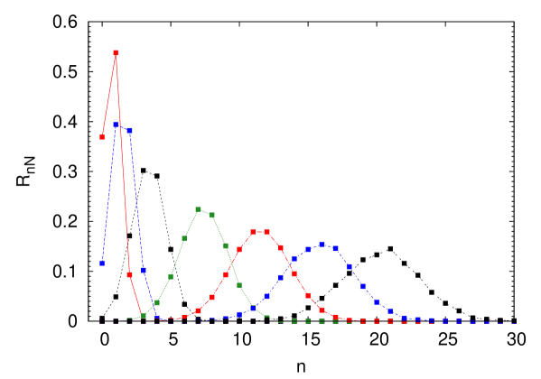
  Figure 1: Conditional normalised multiplicity distribution (relative frequency) of the number of positive pions $n$ in restricted azimuthal region ${\mathcal{A}}=\{20^{\circ}\leq|\phi|\leq 160^{\circ}\}$ for respectively fixed charged multiplicity $N=$ 3, 5, 10, 20, 30, 40, 50, for the UA1 dataset used in Ref. [64]. In accordance with Eq. (6), ${\left\langle n\right\rangle}_{\!\!\scriptscriptstyle N}\simeq 0.39N$.

• Generalisation: While in this paper the analysis will be carried out for the $n(a)$ positive pions of event $a$ falling into ${\mathcal{A}}$, the same formalism obviously applies to negative pions and may equally refer to any other particles such as kaons, baryons, photons etc in any combination which depends on $N$. There is no a priori connection between the definitions of $N$ and $n$.

• Identical-particle vs multi-species analysis: While we do not develop the formalism for correlations between two or three particles of different species or charge, the methodology developed here can be easily modified to deal with such cases. For example, positive-negative pion combinations and “charge balance correlations” [65] can be handled by inserting delta functions $\delta(c,c_{i}^{a})$, where $c$ is the desired charge and $c_{i}^{a}$ the measured charge of track $i$ in event $a$, into the definitions of the counters in Section 2.3.

2.3 Counters and densities for fixed $N$

This section is based on an old formalism [62, 63, 53] which must, however, be updated to accommodate the issues being considered here. The basic building block of correlation analysis is the counter; it is a particular projection of the raw data particular suited to the construction of histograms. Eventwise counters $\hat{\rho}$ for a given event $a$ are averaged to give sample counters $\rho$.

We take the simple case where event $a$ contains $N(a)$ tracks with three-momenta ${\bm{P}}^{a}=\{{\bm{P}}_{1}^{a},\ldots,{\bm{P}}_{N(a)}^{a}\}$, no discrete attributes ${\bm{s}}$ and no further cuts or selection. For each point ${\bm{p}}_{1}$ in momentum space, only that particle $i$ (if any) whose momentum ${\bm{P}}_{i}^{a}$ happens to coincide with ${\bm{p}}$ is to be counted,

$$\hat{\rho}({\bm{p}}_{1}\,|\,{\bm{P}}^{a})=\sum_{i=1}^{N(a)}\delta({\bm{p}}_{1}-{\bm{P}}_{i}^{a}).$$ (7)

Such counters always appear under an integral over some region of the ${\bm{P}}$-space, so that the delta functions fulfil the purpose of counting those particles falling within that region. Alternatively, one can consider the delta functions here and below to represent small nonoverlapping intervals around the specified momenta. The integral over the full momentum space $\Omega$ yields

$$\int_{\Omega}d{\bm{p}}_{1}\,\hat{\rho}({\bm{p}}_{1}\,|\,{\bm{P}}^{a})=N(a)$$ (8)

while an integral over some subspace or bin $\Omega_{b}\subset\Omega$ will yield the number of particles of event $a$ in bin $\Omega_{b}$. The second-order eventwise counter for event $a$ is

$$\hat{\rho}({\bm{p}}_{1},{\bm{p}}_{2}\,|\,{\bm{P}}^{a})=\sum_{i\neq j=1}^{N(a)}\delta({\bm{p}}_{1}-{\bm{P}}_{i}^{a})\,\delta({\bm{p}}_{2}-{\bm{P}}_{j}^{a}),$$ (9)

with the inequality $i\neq j$ ensuring that a single particle is not counted as a “pair”. The counter integrates to

$$\int_{\Omega}d{\bm{p}}_{1}\,d{\bm{p}}_{2}\,\hat{\rho}({\bm{p}}_{1},{\bm{p}}_{2}\,|\,{\bm{P}}^{a}) =N(a)(N(a)-1)\ =\ N(a)^{{\underline{2}}}$$ (10)

using the falling factorial notation

$$N^{{\underline{r}}}=N(N-1)\cdots(N-r+1)\qquad r=1,2,\ldots$$ (11)

as contrasted to the rising factorial (Pochhammer symbol) $N^{\overline{r}}=N(N+1)\cdots(N+r-1)$. The single-particle counter is a projection of $\hat{\rho}({\bm{p}}_{1},{\bm{p}}_{2}\,|\,{\bm{P}}^{a})$ because

$$\int_{\Omega}d{\bm{p}}_{2}\,\hat{\rho}({\bm{p}}_{1},{\bm{p}}_{2}\,|\,{\bm{P}}^{a})=[N(a)-1]\,\hat{\rho}({\bm{p}}_{1}\,|\,{\bm{P}}^{a}).$$ (12)

The most general eventwise counter which enters the exclusive cross section for events with charged multiplicity $N(a)$

$$\hat{\rho}({\bm{p}}_{1},{\bm{p}}_{2},\ldots,{\bm{p}}_{N(a)}\,|\,{\bm{P}}^{a})=\sum_{i_{1}\neq i_{2}\neq\cdots\neq i_{N(a)}=1}^{N(a)}\;\prod_{d=1}^{N(a)}\delta({\bm{p}}_{d}-{\bm{P}}_{i_{d}}^{a})$$ (13)

fully describes the event, including any and all correlations between its particles. It integrates to the factorial of the event multiplicity

$$\int_{\Omega}d{\bm{p}}_{1}\,d{\bm{p}}_{2}\,\cdots\,d{\bm{p}}_{N(a)}\;\hat{\rho}({\bm{p}}_{1},{\bm{p}}_{2},\ldots,{\bm{p}}_{N(a)}\,|\,{\bm{P}}^{a})=N(a)!$$ (14)

and contains all counters of lower order by projection. An $r$th-order counter $\hat{\rho}({\bm{p}}_{1},{\bm{p}}_{2},\ldots,{\bm{p}}_{r}\,|\,{\bm{P}}^{a})$ is zero whenever there are more observation points than particles being observed, $r>N(a)$.

To distinguish eventwise counters for nonfixed $N$ from eventwise counters for fixed $N$, we define the separate eventwise counter for fixed $N$ by specifying an additional Kronecker delta,

$$\hat{\rho}({\bm{p}}_{1},\ldots,{\bm{p}}_{r}\,|\,{\bm{P}}^{a},N) =\delta(N,N(a))\sum_{i_{1}\neq\cdots\neq i_{r}}^{N}\prod_{d}\delta({\bm{p}}_{d}-{\bm{P}}_{i_{d}}^{a})\qquad r=1,2,\ldots,N.$$ (15)

While the counters and densities defined above and below are clearly frame-dependent, it is easy to define corresponding Lorentz-invariant versions by supplementing each delta function in 3-momenta with the corresponding energy; thus Eq. (7) would become, for example,

$$\hat{\rho}({\bm{p}}_{1}\,|\,{\bm{P}}^{a})=\sum_{i=1}^{N(a)}E({\bm{p}}_{1})\,\delta({\bm{p}}_{1}-{\bm{P}}_{i}^{a})$$ (16)

with $E({\bm{p}}_{1})=E_{1}=\sqrt{{\bm{p}}_{1}^{2}+m^{2}}$ the on-shell energy, and in general

$$\hat{\rho}({\bm{p}}_{1},{\bm{p}}_{2},\ldots,{\bm{p}}_{r}\,|\,{\bm{P}}^{a}) =\qquad\sum_{i_{1}\neq i_{2}\neq\cdots\neq i_{r}=1}^{N(a)}\;\prod_{d=1}^{N(a)}E_{d}\,\delta({\bm{p}}_{d}-{\bm{P}}_{i_{d}}^{a})\quad r=1,\ldots,N(a),$$ (17)

$$\hat{\rho}({\bm{p}}_{1},\ldots,{\bm{p}}_{r}\,|\,{\bm{P}}^{a},N) =\delta(N,N(a))\sum_{i_{1}\neq\cdots\neq i_{r}}^{N}\prod_{d}E_{d}\,\delta({\bm{p}}_{d}-{\bm{P}}_{i_{d}}^{a})\quad r=1,\ldots,N,$$ (18)

which are manifestly invariant. Because such counters and densities are, however, always integrated over some $\Omega_{b}$ by $\prod_{d}(d{\bm{p}}_{d}/E_{d})$, the additional factors $E_{d}$ always cancel and play no role on this level of analysis and will be ignored for the time being. The bin boundaries of $\Omega_{b}$ do, however, remain frame-dependent.

Charge-, spin- or species-specific counters are defined in the same way, i.e. by supplying appropriate Kronecker deltas to the counters; for example the particle counter for pions with charge $c_{1}$ at ${\bm{p}}_{1}$ for fixed $N$ is

$$\hat{\rho}({\bm{p}}_{1}\,|\,c_{1},{\bm{P}}^{a},N) =\delta(N,N(a))\,\sum_{i=1}^{N(a)}\delta(c_{1},c_{i}^{a})\,\delta({\bm{p}}_{1}-{\bm{P}}_{i}^{a})\,$$ (19)

while the two-particle counter for charge combination $(c_{1},c_{2})$ at momenta $({\bm{p}}_{1},{\bm{p}}_{2})$ for any $N$ is, for example,

$$\hat{\rho}({\bm{p}}_{1},{\bm{p}}_{2}\,|\,c_{1},c_{2},{\bm{P}}^{a}) =\sum_{i,j=1}^{N(a)}\delta(c_{1},c_{i}^{a})\,\delta({\bm{p}}_{1}-{\bm{P}}_{i}^{a})\,\delta(c_{2},c_{j}^{a})\,\delta({\bm{p}}_{2}-{\bm{P}}_{j}^{a}).$$ (20)

In contrast to Eq. (19), charge counters rather than particle counters would be

$$\hat{\rho}_{c}({\bm{p}}_{1}\,|\,c_{1},{\bm{P}}^{a}) =\sum_{i=1}^{N(a)}c_{1}\,\delta(c_{1},c_{i}^{a})\,\delta({\bm{p}}_{1}-{\bm{P}}_{i}^{a})\,$$ (21)

so that $\hat{\rho}_{c}({\bm{p}}_{1}\,|\,{+}1,{\bm{P}}^{a})+\hat{\rho}_{c}({\bm{p}}_{1}\,|\,{-}1,{\bm{P}}^{a})$ represents the net charge of event $a$ at ${\bm{p}}_{1}$. The two-particle counter for charges $(c_{1},c_{2})$ at momenta $({\bm{p}}_{1},{\bm{p}}_{2})$ is

$$\hat{\rho}^{c_{1}\,c_{2}}\ \equiv\ \hat{\rho}_{c}({\bm{p}}_{1},{\bm{p}}_{2}\,|\,c_{1},c_{2},{\bm{P}}^{a}) =\sum_{i,j=1}^{N(a)}c_{1}\,\delta(c_{1},c_{i}^{a})\,\delta({\bm{p}}_{1}-{\bm{P}}_{i}^{a})\,c_{2}\,\delta(c_{2},c_{j}^{a})\,\delta({\bm{p}}_{2}-{\bm{P}}_{j}^{a}),$$ (22)

and “charge flow” correlations can be constructed from this (for rapidities $(y,y^{\prime})$ in the case of Ref. [66]) such as

$$\Phi(y,y^{\prime}) =-\langle\textstyle\sum_{i\neq j}c_{i}^{a}\,c_{j}^{a}\,\delta(y-Y_{i}^{a})\,\delta(y^{\prime}-Y_{j}^{a})\rangle$$ (23)

which can be expressed as $\Phi=\langle\hat{\rho}^{+-}+\hat{\rho}^{+-}-\hat{\rho}^{++}-\hat{\rho}^{--}\rangle$ and the related “charge balance functions” described in e.g. [46].

Returning to the fixed-$N$ case: eventwise counters will usually be combined with similar events to form event averages. The simplest average is the fixed-$N$ density for the subsample of fixed ${{\mathcal{S}}_{\scriptscriptstyle N}}$,

$$\rho({\bm{p}}_{1}\,|\,{{\mathcal{S}}_{\scriptscriptstyle N}}) =\frac{1}{{{\mathcal{E}}_{\scriptscriptstyle N}}}\sum_{a}\hat{\rho}({\bm{p}}_{1}\,|\,{\bm{P}}^{a},N),$$ (24)

with the Kronecker delta in (15) ensuring that only events in ${{\mathcal{S}}_{\scriptscriptstyle N}}$ are considered, so we need not further specify the individual terms or limits of the $a$-sum. Using (2), it is immediately clear that

$$\int_{\Omega}d{\bm{p}}_{1}\,\rho({\bm{p}}_{1}\,|\,{{\mathcal{S}}_{\scriptscriptstyle N}}) =N$$ (25)

compared to the integral over the corresponding eventwise counter

$$\int_{\Omega}d{\bm{p}}\,\hat{\rho}({\bm{p}}\,|\,{\bm{P}}^{a},N) =N\,\delta(N,N(a))$$ (26)

and to the integral (8); similarly

$$\int_{\Omega}d{\bm{p}}_{1}\cdots d{\bm{p}}_{r}\,\rho({\bm{p}}_{1},\ldots,{\bm{p}}_{r}\,|\,{{\mathcal{S}}_{\scriptscriptstyle N}})=N(N{-}1)\cdots(N{-}r+1)=N^{{\underline{r}}}.$$ (27)

The inclusive averaged density $\rho({\bm{p}}_{1}\,|\,{\mathcal{S}})$ is the weighted average over all $N$ of the fixed-$N$ averages,

$$\rho({\bm{p}}_{1}\,|\,{\mathcal{S}})=\sum_{N=1}^{\infty}{{\mathcal{R}}_{\scriptscriptstyle N}}\,\rho({\bm{p}}_{1}\,|\,{{\mathcal{S}}_{\scriptscriptstyle N}}).$$ (28)

Using (3),(15) and (24), this can be written as

$$\rho({\bm{p}}_{1}\,|\,{\mathcal{S}})=\frac{1}{{{\mathcal{E}}}}\sum_{a}\sum_{i}\delta({\bm{p}}_{1}-{\bm{P}}_{i}^{a}),$$ (29)

and for general $r=1,2,\ldots$

$$\rho({\bm{p}}_{1},\ldots,{\bm{p}}_{r}\,|\,{\mathcal{S}})=\sum_{N=r}^{\infty}{{\mathcal{R}}_{\scriptscriptstyle N}}\,\rho({\bm{p}}_{1},\ldots,{\bm{p}}_{r}\,|\,{{\mathcal{S}}_{\scriptscriptstyle N}})=\frac{1}{{{\mathcal{E}}}}\sum_{a}\sum_{i_{1}\neq\cdots\neq i_{r}}\prod_{d=1}^{r}\delta({\bm{p}}_{d}-{\bm{P}}_{i_{d}}^{a}),$$ (30)

keeping in mind that $\hat{\rho}({\bm{p}}_{1},\ldots,{\bm{p}}_{r}\,|\,{{\mathcal{S}}_{\scriptscriptstyle N}})$ will be zero whenever $N(a)<r$. The integral of any $r$th order inclusive averaged density is the $r$th-order factorial moment of the multiplicity distribution,

$$\int_{\Omega}d{\bm{p}}_{1}\cdots d{\bm{p}}_{r}\,\rho({\bm{p}}_{1},\ldots,{\bm{p}}_{r}\,|\,{\mathcal{S}})=\sum_{N=r}^{\infty}{{\mathcal{R}}_{\scriptscriptstyle N}}\,N^{{\underline{r}}}=\left\langle N^{{\underline{r}}}\right\rangle$$ (31)

with simple angle brackets denoting inclusive averaging.

The averaged counters are of course directly related to the traditional definitions in terms of cross sections. If ${\cal L}$ is the integrated luminosity of incoming particles, the topological cross section is $\sigma_{\scriptscriptstyle N}={{\mathcal{E}}_{\scriptscriptstyle N}}/{\cal L}$, the inelastic cross section is $\sigma_{\scriptscriptstyle I}={{\mathcal{E}}}/{\cal L}$ and the inclusive cross section is $\sigma_{\rm incl}=\sum_{\scriptscriptstyle N}N\sigma_{\scriptscriptstyle N}=\langle N\rangle\,\sigma_{\scriptscriptstyle I}$ while the relative frequency (multiplicity distribution) can be written as usual as ${{\mathcal{R}}_{\scriptscriptstyle N}}=\sigma_{\scriptscriptstyle N}/\sigma_{\scriptscriptstyle I}$. The relation between the differential cross sections and our counters is

$$\rho_{\rm incl}({\bm{p}}_{1},\ldots,{\bm{p}}_{\scriptscriptstyle N})\ =\ \rho({\bm{p}}_{1},\ldots,{\bm{p}}_{\scriptscriptstyle N}\,|\,{\mathcal{S}}) =\frac{1}{\sigma_{\scriptscriptstyle I}}\frac{d^{3N}\sigma_{\rm incl}}{d{\bm{p}}_{1}\cdots d{\bm{p}}_{\scriptscriptstyle N}},$$ (32)

$$\rho({\bm{p}}_{1},\ldots,{\bm{p}}_{\scriptscriptstyle N}\,|\,{{\mathcal{S}}_{\scriptscriptstyle N}}) =\frac{1}{\sigma_{\scriptscriptstyle N}}\frac{d^{3N}\sigma_{\rm excl}}{d{\bm{p}}_{1}\cdots d{\bm{p}}_{\scriptscriptstyle N}},$$ (33)

and so as usual inclusive and exclusive densities are related by [14]

$$\rho({\bm{p}}_{1},\ldots,{\bm{p}}_{\scriptscriptstyle N}\,|\,{\mathcal{S}})=\sum_{N=r}^{\infty}\frac{{{\mathcal{R}}_{\scriptscriptstyle N}}}{(N-r)!}\int\rho({\bm{p}}_{1},\ldots,{\bm{p}}_{\scriptscriptstyle N}\,|\,{{\mathcal{S}}_{\scriptscriptstyle N}})\,d{\bm{p}}_{r+1}\cdots d{\bm{p}}_{\scriptscriptstyle N},$$ (34)

while the semi-inclusive cross sections and counters follow by the usual projections.

2.4 Counters and densities for fixed $(N,{n})$

Our choice of a basic counter is motivated by the experimental situation set out in Section 1: we wish to work in event subsamples of fixed total charged multiplicity $N(a)$ in the entire momentum space $\Omega$, but do the differential correlation analysis using only those pions ${n}$ which fall into the restricted space ${\mathcal{A}}$ and of a particular charge $+1$ or $-1$. This requires the use of “subsubsamples” for which both $N$ and ${n}$ are kept fixed,

$${{\mathcal{S}}_{{n}{\scriptscriptstyle N}}} =\bigl{\{}{\bm{P}}^{a},\text{ with $a$ constrained by }\delta({n},{n_{\scriptscriptstyle+}}(a))\;\delta(N,N(a))\bigr{\}}$$ (35)

with ${n_{\scriptscriptstyle+}}(a)$ the number of positive pions of event $a$ in ${\mathcal{A}}$, and eventwise subsubsample counters

$$\hat{\rho}({\bm{p}}_{1},\ldots,{\bm{p}}_{r}\,|\,{n},N,{\bm{P}}^{a}) =\delta({n},{n_{\scriptscriptstyle+}}(a))\,\delta(N,N(a))\,\sum_{i_{1}\neq\cdots\neq i_{r}=1}^{n}\delta({\bm{p}}_{1}-{\bm{P}}_{i_{1}}^{a})\,\cdots\delta({\bm{p}}_{r}-{\bm{P}}_{i_{r}}^{a})\,.$$ (36)

As in Eq. (2), the number of events in a subsubsample ${{\mathcal{E}}_{{n}{\scriptscriptstyle N}}}=\sum_{a}\delta({n},{n_{\scriptscriptstyle+}}(a))\,\delta(N,N(a))$ enters the relevant event averages

$$\rho({\bm{p}}_{1},\ldots,{\bm{p}}_{r}\,|\,{{\mathcal{S}}_{{n}{\scriptscriptstyle N}}}) =\frac{1}{{{\mathcal{E}}_{{n}{\scriptscriptstyle N}}}}\sum_{a}\hat{\rho}({\bm{p}}_{1},\ldots,{\bm{p}}_{r}\,|\,{n},N,{\bm{P}}^{a})$$ (37)

where once again the double Kronecker deltas in (36) ensure selection of events in ${{\mathcal{S}}_{{n}{\scriptscriptstyle N}}}$ only. Integrals of the counters over the good-azimuth region ${\mathcal{A}}$ yield, for the eventwise and ${{\mathcal{S}}_{{n}{\scriptscriptstyle N}}}$-averaged counters,

$$\int_{\mathcal{A}}d{\bm{p}}_{1}\cdots d{\bm{p}}_{r}\;\hat{\rho}({\bm{p}}_{1},\ldots,{\bm{p}}_{r}\,|\,{n},N,{\bm{P}}^{a}) ={n}^{{\underline{r}}}\;\delta({n},{n_{\scriptscriptstyle+}}(a))\;\delta(N,N(a))$$ (38)

$$\int_{\mathcal{A}}d{\bm{p}}_{1}\cdots d{\bm{p}}_{r}\;\rho({\bm{p}}_{1},\ldots,{\bm{p}}_{r}\,|\,{{\mathcal{S}}_{{n}{\scriptscriptstyle N}}}) ={n}^{{\underline{r}}}.$$ (39)

Bearing in mind that observation points ${\bm{p}}_{1},{\bm{p}}_{2},\ldots$ refer to positive pions in ${\mathcal{A}}$ only, the event-averaged counters for fixed $N$ but any ${n}$ are given by the average weighted in terms of the relative frequency ${{\mathcal{R}}_{{n}{\scriptscriptstyle N}}}={{\mathcal{E}}_{{n}{\scriptscriptstyle N}}}/{{\mathcal{E}}_{\scriptscriptstyle N}}$,

$$\rho({\bm{p}}_{1},\ldots,{\bm{p}}_{r}\,|\,{{\mathcal{S}}_{\scriptscriptstyle N}}) =\sum_{{n}=r}^{N}{{\mathcal{R}}_{{n}{\scriptscriptstyle N}}}\;\rho({\bm{p}}_{1},\ldots,{\bm{p}}_{r}\,|\,{{\mathcal{S}}_{{n}{\scriptscriptstyle N}}})={\left\langle\rho({\bm{p}}_{1},\ldots,{\bm{p}}_{r}\,|\,{{\mathcal{S}}_{{n}{\scriptscriptstyle N}}})\right\rangle}_{\!\!\scriptscriptstyle N}$$ (40)

for $r=1,2,3,\ldots$, which integrate to

$$\int_{\mathcal{A}}d{\bm{p}}_{1}\cdots d{\bm{p}}_{r}\;\rho({\bm{p}}_{1},\ldots,{\bm{p}}_{r}\,|\,{{\mathcal{S}}_{\scriptscriptstyle N}})={\left\langle n^{{\underline{r}}}\right\rangle}_{\!\!\scriptscriptstyle N}.$$ (41)

3 Construction of correlation quantities

3.1 Criteria

Correlation measurements of any sort are only meaningful if a reference baseline signifying “independence” or “lack of correlation” is defined quantitatively; indeed, many different kinds of correlations may be defined and measured on the same data, depending on which particular physical and mathematical scenario is considered to be known or trivial and taken to be the baseline [61]. In our case, we require the reference distribution to have the following properties:

1. The number of charged pions in all phase space $N$ is an important parameter as a measure of possibly different physics, but only the $n$ positive pions in ${\mathcal{A}}$ are to be considered in the differential analysis.

2. For a given $(N,n)$, the momenta of the reference density $\rho^{\rm ref}({\bm{p}}_{1},\ldots,{\bm{p}}_{r}\,|\,{{\mathcal{S}}_{{n}{\scriptscriptstyle N}}})$ should be mutually independent for any order $1\leq r\leq n$. This and the previous requirement imply that the reference should be a $n$-multinomial distributed over continuous momentum space; see Section 3.2.1.

3. Given fixed $N$, the reference density $\rho^{\rm ref}({\bm{p}}_{1},\ldots,{\bm{p}}_{r}\,|\,{{\mathcal{S}}_{\scriptscriptstyle N}})$ must reproduce the $n$-multiplicity structure of the subsubsamples ${{\mathcal{S}}_{{n}{\scriptscriptstyle N}}}$ as embodied in ${{\mathcal{R}}_{{n}{\scriptscriptstyle N}}}$. As set out further in Section 3.2.2, this translates into an average of multinomials,

   $$\rho^{\rm ref}({\bm{p}}_{1},\ldots,{\bm{p}}_{r}\,|\,{{\mathcal{S}}_{\scriptscriptstyle N}}) =\sum_{{n}=r}^{N}{{\mathcal{R}}_{{n}{\scriptscriptstyle N}}}\;\rho^{\rm mult}({\bm{p}}_{1},\ldots,{\bm{p}}_{r}\,|\,\bm{\alpha},{{\mathcal{S}}_{{n}{\scriptscriptstyle N}}})={\left\langle\rho^{\rm mult}({\bm{p}}_{1},\ldots,{\bm{p}}_{r}\,|\,\bm{\alpha},{{\mathcal{S}}_{{n}{\scriptscriptstyle N}}})\right\rangle}_{\!\!\scriptscriptstyle N}.$$ (42)

4. The reference density should reproduce the measured one-particle density in momentum space. This can in principle be satisfied by three different expressions for the multinomial’s parameters ${\bm{\alpha}}$: see Section 3.2.3.

5. Measures of correlation must reduce to zero even on a differential basis whenever the data is, in fact, uncorrelated. While this may seem self-evident, this requirement is often ignored or not satisfied in the literature. We address the resulting proper baseline through the use of internal cumulants in Section 3.3.

6. The measure of correlation should be insensitive to the one-particle distribution. This is addressed as usual by normalisation; see Section 3.3.

3.2 The reference distribution

3.2.1 Multinomials in discrete and continuous spaces

Before Eq. (42) can be developed further, it is necessary to take a detour into discrete outcome spaces before tackling the continuous outcome space defined by ${\bm{p}}$ and ${\bm{P}}^{a}$. The reason is that multinomial distributions for continuous arguments ${\bm{p}}$ can be written only as a limit of the discrete precursor.

Let there be bins $\Omega_{b},b=1,\ldots,B$ with the corresponding set of Bernoulli probabilities ${\bm{\alpha}}=\{\alpha(b)\}_{b=1}^{B}$ of a single particle falling into bin $\Omega_{b}$, normalised by $\sum_{b}\alpha(b)=1$. Independent tossing of $n$ particles into these bins results in the multinomial for the bin counts ${\bm{n}}=\{n_{b}\}_{b=1}^{B}$,

$$p({\bm{n}}\,|\,{\bm{\alpha}},n) =n!\prod_{b=1}^{B}\frac{\alpha(b)^{n_{b}}}{n_{b}!},$$ (43)

with normalisation

$$\sum_{U({\bm{n}})}p({\bm{n}}\,|\,{\bm{\alpha}},n) =1,$$ (44)

where the sum must be taken over the “universal set”

$$U({\bm{n}})=\{{\bm{n}}\,|\,n_{b}\geq 0;\;\textstyle\sum_{b}n_{b}=n\}.$$ (45)

The multivariate factorial moment generating function (FMGF) for this multinomial for the set of source parameters ${\bm{\lambda}}=\{\lambda(b)\}_{b=1}^{B}$ can be solved in closed form,

$$Q^{\rm mult}({\bm{\lambda}}\,|\,{\bm{\alpha}},n) =\sum_{U}p({\bm{n}}\,|\,{\bm{\alpha}},n)\;\prod_{b}(1-\lambda(b))^{n_{b}}\ =\ \biggl{[}1-\sum_{b}\lambda(b)\alpha(b)\biggr{]}^{n}.$$ (46)

The FMGF $Q({\bm{\lambda}})$ can generally be used to find multivariate factorial moments $\rho(b_{i_{1}},b_{i_{2}},\cdots,b_{i_{r}})$ and factorial cumulants $\kappa(b_{i_{1}},b_{i_{2}},\cdots,b_{i_{r}})$ for any selection of bins $(b_{i_{1}},b_{i_{2}},\cdots,b_{i_{r}})\in(1,\ldots,B)$, including repeated indices, by differentiation

$$\rho(b_{i_{1}},b_{i_{2}},\cdots,b_{i_{r}}) =\frac{(-1)^{r}\;\partial^{r}Q({\bm{\lambda}})}{\partial\lambda(b_{i_{1}})\;\partial\lambda(b_{i_{2}})\,\cdots\,\partial\lambda(b_{i_{r}})}\biggr{|}_{{\bm{\lambda}}=0},$$ (47)

$$\kappa(b_{i_{1}},b_{i_{2}},\cdots,b_{i_{r}}) =\frac{(-1)^{r}\;\partial^{r}\ln Q({\bm{\lambda}})}{\partial\lambda(b_{i_{1}})\;\partial\lambda(b_{i_{2}})\,\cdots\,\partial\lambda(b_{i_{r}})}\biggr{|}_{{\bm{\lambda}}=0}.$$ (48)

For the multinomial case (46), the factorial moments and cumulants are therefore

$$\rho^{\rm mult}(b_{i_{1}},b_{i_{2}},\cdots,b_{i_{r}}\,|\,{\bm{\alpha}},n) =n^{{\underline{r}}}\;\prod_{d=1}^{r}\alpha(i_{d})\qquad\forall\;r\leq n,$$ (49)

$$\kappa^{\rm mult}(b_{i_{1}},b_{i_{2}},\cdots,b_{i_{r}}\,|\,{\bm{\alpha}},n) =(-1)^{r-1}\,(r-1)!\cdot n\prod_{d=1}^{r}\alpha(i_{d}).$$ (50)

The multinomial for variable ${\bm{p}}$ in continuous outcome space $\mathbb{R}$ is derived by keeping $n$ constant while taking the limit $B\to\infty$ with bin sizes tending to zero and changing to a Bernoulli probability density $\alpha(b)\to d{\bm{p}}\,\alpha({\bm{p}})$ normalised by $\int_{\mathcal{A}}d{\bm{p}}\,\alpha({\bm{p}})=1$. The result is the point process where the probability for the count $n({\bm{p}})$ in the infinitesimal “bin” around any ${\bm{p}}$ to be larger than 1 becomes negligible, i.e. we have at most one particle at a given ${\bm{p}}$. While the multinomial probability itself can be written only as a limit, the FMGF can be written analytically as the functional [67]

$$Q^{\rm mult}[\lambda({\bm{p}})\,|\,\alpha({\bm{p}}),n]=\left[1-\int_{\mathcal{A}}d{\bm{p}}\,\lambda({\bm{p}})\,\alpha({\bm{p}})\right]^{n}.$$ (51)

Factorial moments and factorial cumulants are found generically from functional derivatives [14]

$$\rho({\bm{p}}_{i_{1}},{\bm{p}}_{i_{2}},\cdots,{\bm{p}}_{i_{r}}) =\frac{(-1)^{r}\;\delta^{r}Q[\lambda({\bm{p}})]}{\delta\lambda({\bm{p}}_{i_{1}})\;\delta\lambda({\bm{p}}_{i_{2}})\;\cdots\delta\lambda({\bm{p}}_{i_{r}})\;}\biggr{|}_{\lambda({\bm{p}})=0},$$ (52)

$$\kappa({\bm{p}}_{i_{1}},{\bm{p}}_{i_{2}},\cdots,{\bm{p}}_{i_{r}}) =\frac{(-1)^{r}\;\delta^{r}\ln Q[\lambda({\bm{p}})]}{\delta\lambda({\bm{p}}_{i_{1}})\;\delta\lambda({\bm{p}}_{i_{2}})\;\cdots\delta\lambda({\bm{p}}_{i_{r}})\;}\biggr{|}_{\lambda({\bm{p}})=0},$$ (53)

which for the multinomial $Q[{\bm{\lambda}}({\bm{p}})]=Q^{\rm mult}[\lambda({\bm{p}})\,|\,\alpha({\bm{p}}),n]$ of (51) yield

$$\rho^{\rm mult}({\bm{p}}_{i_{1}},{\bm{p}}_{i_{2}},\cdots,{\bm{p}}_{i_{r}}\,|\,\alpha({\bm{p}}),n) =n^{{\underline{r}}}\;\prod_{k=1}^{r}\alpha({\bm{p}}_{i_{k}})\qquad 1\leq r\leq n,$$ (54)

$$\kappa^{\rm mult}({\bm{p}}_{i_{1}},{\bm{p}}_{i_{2}},\cdots,{\bm{p}}_{i_{r}}\,|\,\alpha({\bm{p}}),n) =(-1)^{r-1}\,(r-1)!\cdot n\prod_{k=1}^{r}\alpha({\bm{p}}_{i_{k}}).$$ (55)

3.2.2 Multinomial reference for fixed $N$

Applying the above general case to our reference distribution (42), we must rewrite Eq. (51) to make provision for the fact that ${\bm{\alpha}}$ may in general depend not only on $N$ but also on $n$,

$$Q^{\rm mult}[\lambda({\bm{p}})\,|\,\alpha({\bm{p}}\,|\,{{\mathcal{S}}_{{n}{\scriptscriptstyle N}}})]=\left[1-\int d{\bm{p}}\,\lambda({\bm{p}})\,\alpha({\bm{p}}\,|\,{{\mathcal{S}}_{{n}{\scriptscriptstyle N}}})\right]^{{n}}.$$ (56)

Inserting (56) into (42), we find the FMGF for the reference distribution of subsample ${{\mathcal{S}}_{\scriptscriptstyle N}}$ to be

$$Q^{\rm ref}[\lambda({\bm{p}})\,|\,\alpha({\bm{p}}),{{\mathcal{S}}_{\scriptscriptstyle N}}] =\sum_{n}{{\mathcal{R}}_{{n}{\scriptscriptstyle N}}}\;Q^{\rm mult}[\lambda({\bm{p}})\,|\,\alpha({\bm{p}}\,|\,{{\mathcal{S}}_{{n}{\scriptscriptstyle N}}})]\ =\ {\left\langle\left[1-\int d{\bm{p}}\,\lambda({\bm{p}})\,\alpha({\bm{p}}\,|\,{{\mathcal{S}}_{{n}{\scriptscriptstyle N}}})\right]^{{n}}\right\rangle}_{\!\!\!\!\scriptscriptstyle N}.$$ (57)

Using (54), the reference factorial moments are therefore,

$$\rho^{\rm ref}({\bm{p}}_{1},{\bm{p}}_{2},\cdots,{\bm{p}}_{r}\,|\,{{\mathcal{S}}_{\scriptscriptstyle N}}) ={\left\langle{n}^{{\underline{r}}}\;\prod_{k=1}^{r}\alpha({\bm{p}}_{k}\,|\,{{\mathcal{S}}_{{n}{\scriptscriptstyle N}}})\right\rangle}_{\!\!\!\!\scriptscriptstyle N}\qquad\forall\;r\leq n$$ (58)

with corresponding expressions for the reference factorial cumulants.

3.2.3 Reproducing the one-particle distribution

The set of functions $\alpha({\bm{p}}\,|\,{{\mathcal{S}}_{{n}{\scriptscriptstyle N}}})$ are as yet undetermined, apart from the general constraints $\alpha({\bm{p}}\,|\,{{\mathcal{S}}_{{n}{\scriptscriptstyle N}}})\geq 0$ and $\int_{\mathcal{A}}d{\bm{p}}\,\alpha({\bm{p}}\,|\,{{\mathcal{S}}_{{n}{\scriptscriptstyle N}}})=1$. In multinomials of all kinds, the Bernoulli probabilities ${\bm{\alpha}}$ are fixed parameters and therefore are the conveyers of whatever remains constant in the outcomes while the detailed outcomes fluctuate as statistical outcomes do. The “field” $\alpha({\bm{p}}\,|\,{{\mathcal{S}}_{{n}{\scriptscriptstyle N}}})$ can and must therefore be seen as the quantity encompassing the “physics” of the one-particle distributions, which, in the absence of additional external information, is embodied by our experimental data sample: the experimental densities $\rho({\bm{p}}_{1},\ldots,{\bm{p}}_{\scriptscriptstyle N}\,|\,{{\mathcal{S}}_{\scriptscriptstyle N}})$ “are” the physics, including all correlations, and their first-order projections $\rho({\bm{p}}_{1}\,|\,{{\mathcal{S}}_{\scriptscriptstyle N}})$ “are” the one-particle physics. The question immediately arises whether $\alpha({\bm{p}}\,|\,{{\mathcal{S}}_{{n}{\scriptscriptstyle N}}})$ should be fixed by $\rho({\bm{p}}\,|\,{{\mathcal{S}}_{{n}{\scriptscriptstyle N}}})$ or the $n$-average $\rho({\bm{p}}\,|\,{{\mathcal{S}}_{\scriptscriptstyle N}})={\left\langle\rho({\bm{p}}\,|\,{{\mathcal{S}}_{{n}{\scriptscriptstyle N}}})\right\rangle}_{\!\!\scriptscriptstyle N}$. Three possible choices come to mind:

1. It is tempting to define it in terms of the density for each subsubsample ${{\mathcal{S}}_{{n}{\scriptscriptstyle N}}}$,

   $$\alpha({\bm{p}}\,|\,{{\mathcal{S}}_{{n}{\scriptscriptstyle N}}}) =\frac{\rho({\bm{p}}\,|\,{{\mathcal{S}}_{{n}{\scriptscriptstyle N}}})}{n}\qquad\forall\;(N,n),$$ (59)

   which is correctly normalised since $\int d{\bm{p}}\,\rho({\bm{p}}\,|\,{{\mathcal{S}}_{{n}{\scriptscriptstyle N}}})=n$. As this choice would attribute physical significance to $n$, it would be appropriate whenever $n$ is associated with additionally measured experimental information. If, however, $n$ fluctuates randomly from event to event based in part on unmeasured or unmeasurable properties such as an event’s azimuthal orientation, use of (59) makes no sense.

   If $n$ is deemed physically relevant, correlations in terms of $\rho({\bm{p}}_{1},\ldots,{\bm{p}}_{r}\,|\,{{\mathcal{S}}_{{n}{\scriptscriptstyle N}}})$ of Eq. (37) may be feasible, conditional on the availability of a sufficient number of events ${{\mathcal{E}}_{{n}{\scriptscriptstyle N}}}$. Where sample sizes do not permit this, one could nevertheless attempt to measure what have historically been termed “short-range correlations” but in this case not in the traditional sense of fixed-$N$ correlations versus inclusive ones, but rather of fixed-$n$-fixed-$N$ correlations versus fluctuating-$n$-fixed-$N$ correlations. See Section 3.6.

2. A second choice

   $$\alpha({\bm{p}}\,|\,{{\mathcal{S}}_{{n}{\scriptscriptstyle N}}}) ={\left\langle\frac{\rho({\bm{p}}\,|\,{{\mathcal{S}}_{{n}{\scriptscriptstyle N}}})}{n}\right\rangle}_{\!\!\!\!\scriptscriptstyle N}$$ (60)

   would be properly normalised but fails to satisfy the crucial relations (78)–(80) below and is hence discarded.

3. While remaining open-minded towards Choice 1, we therefore choose the third possibility, the ratio of the average density divided by the average, all for fixed $N$,

   $$\alpha({\bm{p}}\,|\,{{\mathcal{S}}_{{n}{\scriptscriptstyle N}}}) =\frac{{\left\langle\rho({\bm{p}}\,|\,{{\mathcal{S}}_{{n}{\scriptscriptstyle N}}})\right\rangle}_{\!\!\scriptscriptstyle N}}{{\left\langle n\right\rangle}_{\!\!\scriptscriptstyle N}}=\frac{\rho({\bm{p}}\,|\,{{\mathcal{S}}_{\scriptscriptstyle N}})}{{\left\langle n\right\rangle}_{\!\!\scriptscriptstyle N}}$$ (61)

   which would be appropriate for samples where ${{\mathcal{E}}_{{n}{\scriptscriptstyle N}}}$ is too small or physical significance can be attributed only to $N$ but not to $n$. According to (41), it is also correctly normalised and ensures that the Bernoulli parameters are the same for all events in ${{\mathcal{S}}_{\scriptscriptstyle N}}$, independent of $n$. Substituting this into Eq. (58), the differential reference factorial moments orders become

   $$\rho^{\rm ref}({\bm{p}}_{1},{\bm{p}}_{2},\cdots,{\bm{p}}_{r}\,|\,{{\mathcal{S}}_{\scriptscriptstyle N}}) =\frac{{\left\langle n^{{\underline{r}}}\right\rangle}_{\!\!\scriptscriptstyle N}}{{\left\langle n\right\rangle}_{\!\!\scriptscriptstyle N}^{r}}\;\prod_{d=1}^{r}\rho({\bm{p}}_{d}\,|\,{{\mathcal{S}}_{\scriptscriptstyle N}})\ =\ F_{r{\scriptscriptstyle N}}\;\prod_{d=1}^{r}\rho({\bm{p}}_{d}\,|\,{{\mathcal{S}}_{\scriptscriptstyle N}})$$ (62)

   where we identify the prefactor as the normalised factorial moments of the $n$-multiplicity distribution for given $N$,

   $$F_{r{\scriptscriptstyle N}}=\frac{{\left\langle n^{{\underline{r}}}\right\rangle}_{\!\!\scriptscriptstyle N}}{{\left\langle n\right\rangle}_{\!\!\scriptscriptstyle N}^{r}},$$ (63)

   while the generating functional (57) becomes (see also [13])

   $$Q^{\rm ref}[\lambda({\bm{p}})\,|\,\alpha({\bm{p}}),{{\mathcal{S}}_{\scriptscriptstyle N}}] ={\left\langle\left[1-\int d{\bm{p}}\,\lambda({\bm{p}})\,\frac{\rho({\bm{p}}\,|\,{{\mathcal{S}}_{\scriptscriptstyle N}})}{{\left\langle n\right\rangle}_{\!\!\scriptscriptstyle N}}\right]^{{n}}\right\rangle}_{\!\!\!\!\scriptscriptstyle N}.$$ (64)

Taking functional derivatives of the logarithm of (64), the first, second and third order cumulants of the reference density are

$$\kappa^{\rm ref}({\bm{p}}_{1}\,|\,{{\mathcal{S}}_{\scriptscriptstyle N}}) =\rho^{\rm ref}({\bm{p}}_{1}\,|\,{{\mathcal{S}}_{\scriptscriptstyle N}})\ =\ \rho({\bm{p}}_{1}\,|\,{{\mathcal{S}}_{\scriptscriptstyle N}})$$ (65)

$$\kappa^{\rm ref}({\bm{p}}_{1},{\bm{p}}_{2}\,|\,{{\mathcal{S}}_{\scriptscriptstyle N}}) =\rho^{\rm ref}({\bm{p}}_{1},{\bm{p}}_{2}\,|\,{{\mathcal{S}}_{\scriptscriptstyle N}})-\rho({\bm{p}}_{1}\,|\,{{\mathcal{S}}_{\scriptscriptstyle N}})\;\rho({\bm{p}}_{2}\,|\,{{\mathcal{S}}_{\scriptscriptstyle N}})$$ (66)

$$=\left(\frac{{\left\langle{n}^{\underline{2}}\right\rangle}_{\!\!\scriptscriptstyle N}}{{\left\langle{n}\right\rangle}_{\!\!\scriptscriptstyle N}^{2}}-1\right)\rho({\bm{p}}_{1}\,|\,{{\mathcal{S}}_{\scriptscriptstyle N}})\,\rho({\bm{p}}_{2}\,|\,{{\mathcal{S}}_{\scriptscriptstyle N}})$$ (67)

$$\kappa^{\rm ref}({\bm{p}}_{1},{\bm{p}}_{2},{\bm{p}}_{3}\,|\,{{\mathcal{S}}_{\scriptscriptstyle N}}) =\rho^{\rm ref}({\bm{p}}_{1},{\bm{p}}_{2},{\bm{p}}_{3}\,|\,{{\mathcal{S}}_{\scriptscriptstyle N}})$$ (68)

$$\quad-[3]\,\rho^{\rm ref}({\bm{p}}_{1},{\bm{p}}_{2}\,|\,{{\mathcal{S}}_{\scriptscriptstyle N}})\rho({\bm{p}}_{3}\,|\,{{\mathcal{S}}_{\scriptscriptstyle N}})+2\rho({\bm{p}}_{1}\,|\,{{\mathcal{S}}_{\scriptscriptstyle N}})\rho({\bm{p}}_{2}\,|\,{{\mathcal{S}}_{\scriptscriptstyle N}})\rho({\bm{p}}_{3}\,|\,{{\mathcal{S}}_{\scriptscriptstyle N}})$$

$$=\left(\frac{{\left\langle{n}^{{\underline{3}}}\right\rangle}_{\!\!\scriptscriptstyle N}}{{\left\langle{n}\right\rangle}_{\!\!\scriptscriptstyle N}^{3}}\;-3\frac{{\left\langle{n}^{{\underline{2}}}\right\rangle}_{\!\!\scriptscriptstyle N}}{{\left\langle{n}\right\rangle}_{\!\!\scriptscriptstyle N}^{2}}+2\right)\rho({\bm{p}}_{1}\,|\,{{\mathcal{S}}_{\scriptscriptstyle N}})\rho({\bm{p}}_{2}\,|\,{{\mathcal{S}}_{\scriptscriptstyle N}})\rho({\bm{p}}_{3}\,|\,{{\mathcal{S}}_{\scriptscriptstyle N}})$$ (69)

where the square bracket $[3]$ indicates the number of distinct permutations which must be taken into account. The terms in the rounded brackets are readily recognised as the normalised factorial cumulants of the ${n}$ distribution for a given fixed $N$

$$K_{r{\scriptscriptstyle N}} =\frac{1}{{\left\langle n\right\rangle}_{\!\!\scriptscriptstyle N}^{r}}\frac{(-\partial)^{r}}{\partial\Lambda^{r}}\ln\left(\sum_{{n}=0}^{N}{{\mathcal{R}}_{{n}{\scriptscriptstyle N}}}\,(1-\Lambda)^{n}\right)_{\Lambda=0},$$ (70)

and so generalisation to arbitrary orders is immediate,

$$\kappa^{\rm ref}({\bm{p}}_{1},\cdots,{\bm{p}}_{r}\,|\,{{\mathcal{S}}_{\scriptscriptstyle N}})=K_{r{\scriptscriptstyle N}}\prod_{k=1}^{r}\rho({\bm{p}}_{k}\,|\,{{\mathcal{S}}_{\scriptscriptstyle N}}).$$ (71)

This can be proven generally by defining the functional $\Lambda[\lambda({\bm{p}})]=\int d{\bm{p}}\,\lambda({\bm{p}})\,\rho({\bm{p}}\,|\,{{\mathcal{S}}_{\scriptscriptstyle N}})/{\left\langle n\right\rangle}_{\!\!\scriptscriptstyle N}$ which has only a first nonzero functional derivative $\delta\Lambda/\delta\lambda({\bm{p}}_{1})=\rho({\bm{p}}\,|\,{{\mathcal{S}}_{\scriptscriptstyle N}})/{\left\langle n\right\rangle}_{\!\!\scriptscriptstyle N}$ and the multiplicity generating function ${\mathcal{Z}}(\Lambda\,|\,{{\mathcal{S}}_{\scriptscriptstyle N}})=\sum_{n}{{\mathcal{R}}_{{n}{\scriptscriptstyle N}}}(1-\Lambda)^{n}$, in terms of which $Q^{\rm ref}[\lambda]={\mathcal{Z}}[\Lambda[\lambda]]$.

3.3 Internal cumulants for fixed ${{\mathcal{S}}_{\scriptscriptstyle N}}$

Eq. (71) shows that the differential cumulants of the reference distribution are directly proportional to the integrated cumulants $K_{r{\scriptscriptstyle N}}$ of $n$, which are zero only if ${{\mathcal{R}}_{{n}{\scriptscriptstyle N}}}$ is poissonian. For fixed $N$, neither the integrated cumulants $K_{r{\scriptscriptstyle N}}$ nor the differential ones are zero. While this has long been recognised in the literature [15], the inevitable consequence was not drawn, namely that “poissonian” cumulants for fixed $N$

$$\kappa({\bm{p}}_{1},{\bm{p}}_{2}\,|\,{{\mathcal{S}}_{\scriptscriptstyle N}}) =\rho({\bm{p}}_{1},{\bm{p}}_{2}\,|\,{{\mathcal{S}}_{\scriptscriptstyle N}})-\rho({\bm{p}}_{1}\,|\,{{\mathcal{S}}_{\scriptscriptstyle N}})\;\rho({\bm{p}}_{2}\,|\,{{\mathcal{S}}_{\scriptscriptstyle N}}),$$ (72)

$$\kappa({\bm{p}}_{1},{\bm{p}}_{2},{\bm{p}}_{3}\,|\,{{\mathcal{S}}_{\scriptscriptstyle N}}) =\rho({\bm{p}}_{1},{\bm{p}}_{2},{\bm{p}}_{3}\,|\,{{\mathcal{S}}_{\scriptscriptstyle N}})$$

$$\quad-[3]\,\rho({\bm{p}}_{1},{\bm{p}}_{2}\,|\,{{\mathcal{S}}_{\scriptscriptstyle N}})\;\rho({\bm{p}}_{3}\,|\,{{\mathcal{S}}_{\scriptscriptstyle N}})+2\rho({\bm{p}}_{1}\,|\,{{\mathcal{S}}_{\scriptscriptstyle N}})\;\rho({\bm{p}}_{2}\,|\,{{\mathcal{S}}_{\scriptscriptstyle N}})\;\rho({\bm{p}}_{3}\,|\,{{\mathcal{S}}_{\scriptscriptstyle N}})$$ (73)

etc. cannot possibly represent true correlations because they are nonzero even when the momenta are fully independent. It is known that the theory of cumulants needs improvement on a fundamental level which reaches well beyond the scope of this paper [68], [69], but those difficulties are irrelevant here. A first step which does address the above concerns was taken in Ref. [18], where it was shown very generally on the basis of generating functionals that correlations for samples of fixed $N$ are best measured using the internal cumulants $\kappa^{I}$, which are defined as the differences between the measured and the reference cumulants of the same order

$$\kappa^{I}({\bm{p}}_{1},\ldots,{\bm{p}}_{r}\,|\,{{\mathcal{S}}_{\scriptscriptstyle N}}) =\kappa({\bm{p}}_{1},\ldots,{\bm{p}}_{r}\,|\,{{\mathcal{S}}_{\scriptscriptstyle N}})-\kappa^{\rm ref}({\bm{p}}_{1},\ldots,{\bm{p}}_{r}\,|\,{{\mathcal{S}}_{\scriptscriptstyle N}}).$$ (74)

For our averaged-multinomial reference case, the internal cumulants of second and third order are given by the differences between Eqs. (72) and (67) and between (3.3) and (69), resulting in

$$\kappa^{I}({\bm{p}}_{1},{\bm{p}}_{2}\,|\,{{\mathcal{S}}_{\scriptscriptstyle N}}) =\rho({\bm{p}}_{1},{\bm{p}}_{2}\,|\,{{\mathcal{S}}_{\scriptscriptstyle N}})-F_{2{\scriptscriptstyle N}}\rho({\bm{p}}_{1}\,|\,{{\mathcal{S}}_{\scriptscriptstyle N}})\;\rho({\bm{p}}_{2}\,|\,{{\mathcal{S}}_{\scriptscriptstyle N}}),$$ (75)

$$\kappa^{I}({\bm{p}}_{1},{\bm{p}}_{2},{\bm{p}}_{3}\,|\,{{\mathcal{S}}_{\scriptscriptstyle N}}) =\rho({\bm{p}}_{1},{\bm{p}}_{2},{\bm{p}}_{3}\,|\,{{\mathcal{S}}_{\scriptscriptstyle N}})-[3]\,\rho({\bm{p}}_{1},{\bm{p}}_{2}\,|\,{{\mathcal{S}}_{\scriptscriptstyle N}})\;\rho({\bm{p}}_{3}\,|\,{{\mathcal{S}}_{\scriptscriptstyle N}})$$

$$\quad+G_{3{\scriptscriptstyle N}}\;\rho({\bm{p}}_{1}\,|\,{{\mathcal{S}}_{\scriptscriptstyle N}})\rho({\bm{p}}_{2}\,|\,{{\mathcal{S}}_{\scriptscriptstyle N}})\rho({\bm{p}}_{3}\,|\,{{\mathcal{S}}_{\scriptscriptstyle N}}),$$ (76)

with

$$G_{3{\scriptscriptstyle N}} =3F_{2{\scriptscriptstyle N}}-F_{3{\scriptscriptstyle N}}\ =\ 3\,\frac{{\left\langle n(n{-}1)\right\rangle}_{\!\!\scriptscriptstyle N}}{{\left\langle n\right\rangle}_{\!\!\scriptscriptstyle N}^{2}}-\frac{{\left\langle n(n{-}1)(n{-}2)\right\rangle}_{\!\!\scriptscriptstyle N}}{{\left\langle n\right\rangle}_{\!\!\scriptscriptstyle N}^{3}}$$ (77)

and so on for higher orders. These internal cumulants are identically zero if and when the measured densities for fixed ${{\mathcal{S}}_{{n}{\scriptscriptstyle N}}}$ are multinomials since then from Eq. (62)

$$\rho({\bm{p}}_{1},{\bm{p}}_{2}\,|\,{{\mathcal{S}}_{\scriptscriptstyle N}}) \rightarrow\rho^{\rm ref}({\bm{p}}_{1},{\bm{p}}_{2}\,|\,{{\mathcal{S}}_{\scriptscriptstyle N}})=F_{2{\scriptscriptstyle N}}\rho({\bm{p}}_{1}\,|\,{{\mathcal{S}}_{\scriptscriptstyle N}})\;\rho({\bm{p}}_{2}\,|\,{{\mathcal{S}}_{\scriptscriptstyle N}})$$ (78)

so that $\kappa^{I}({\bm{p}}_{1},{\bm{p}}_{2}\,|\,{{\mathcal{S}}_{\scriptscriptstyle N}})\rightarrow 0$ whenever the data is multinomial, while

$$\rho({\bm{p}}_{1},{\bm{p}}_{2},{\bm{p}}_{3}\,|\,{{\mathcal{S}}_{\scriptscriptstyle N}})\rightarrow F_{3{\scriptscriptstyle N}}\rho({\bm{p}}_{1}\,|\,{{\mathcal{S}}_{\scriptscriptstyle N}})\rho({\bm{p}}_{2}\,|\,{{\mathcal{S}}_{\scriptscriptstyle N}})\rho({\bm{p}}_{3}\,|\,{{\mathcal{S}}_{\scriptscriptstyle N}})$$ (79)

ensures that $\kappa^{I}({\bm{p}}_{1},{\bm{p}}_{2},{\bm{p}}_{3}\,|\,{{\mathcal{S}}_{\scriptscriptstyle N}})\rightarrow 0$ in the same case. On another level, the internal cumulants always integrate to zero over the full good-azimuth space ${\mathcal{A}}$, irrespective of the presence of correlations,

$$\int_{\mathcal{A}}d{\bm{p}}_{1}\,d{\bm{p}}_{2}\;\kappa^{I}({\bm{p}}_{1},{\bm{p}}_{2}\,|\,{{\mathcal{S}}_{\scriptscriptstyle N}})\ =\ \int_{\mathcal{A}}d{\bm{p}}_{1}\,d{\bm{p}}_{2}\,d{\bm{p}}_{3}\;\kappa^{I}({\bm{p}}_{1},{\bm{p}}_{2},{\bm{p}}_{3}\,|\,{{\mathcal{S}}_{\scriptscriptstyle N}})\ =\ 0$$ (80)

and so on for all orders. Both properties will remain valid after transformation from three-momenta to invariant four-momentum differences in Section 3.4. In the case of Poissonian statistics, $F_{r{\scriptscriptstyle N}}=1\;\forall r$, so that the above internal cumulants revert to their usual definitions.

As stated in Section 3.1, the measured correlations may in addition be made insensitive to the one-particle distribution through normalisation. As set out in Ref. [18], such normalisation is achieved for fixed $N$ by dividing the internal cumulants by the corresponding reference distribution density, which for the case at hand is given by Eq. (62). This leads to the second-order normalised internal cumulant

$$K^{I}({\bm{p}}_{1},{\bm{p}}_{2}\,|\,{{\mathcal{S}}_{\scriptscriptstyle N}}) =\frac{1}{F_{2{\scriptscriptstyle N}}}\;\frac{\rho({\bm{p}}_{1},{\bm{p}}_{2}\,|\,{{\mathcal{S}}_{\scriptscriptstyle N}})}{\rho({\bm{p}}_{1}\,|\,{{\mathcal{S}}_{\scriptscriptstyle N}})\;\rho({\bm{p}}_{2}\,|\,{{\mathcal{S}}_{\scriptscriptstyle N}})}\ -\ 1,$$ (81)

while in third order we get

$$K^{I}({\bm{p}}_{1},{\bm{p}}_{2},{\bm{p}}_{3}\,|\,{{\mathcal{S}}_{\scriptscriptstyle N}}) =\frac{1}{F_{3{\scriptscriptstyle N}}}\left(\frac{\rho({\bm{p}}_{1},{\bm{p}}_{2},{\bm{p}}_{3}\,|\,{{\mathcal{S}}_{\scriptscriptstyle N}})-[3]\,\rho({\bm{p}}_{1},{\bm{p}}_{2}\,|\,{{\mathcal{S}}_{\scriptscriptstyle N}})\;\rho({\bm{p}}_{3}\,|\,{{\mathcal{S}}_{\scriptscriptstyle N}})}{\rho({\bm{p}}_{1}\,|\,{{\mathcal{S}}_{\scriptscriptstyle N}})\rho({\bm{p}}_{2}\,|\,{{\mathcal{S}}_{\scriptscriptstyle N}})\rho({\bm{p}}_{3}\,|\,{{\mathcal{S}}_{\scriptscriptstyle N}})}\right)+3\frac{F_{2{\scriptscriptstyle N}}}{F_{3{\scriptscriptstyle N}}}-1.$$ (82)

3.4 Correlation integrals for momentum differences

In femtoscopy, correlations are mostly expressed in terms of pair variables ${\bm{K}}=\tfrac{1}{2}\left({\bm{p}}_{1}+{\bm{p}}_{2}\right)$ and difference ${\bm{q}}={\bm{p}}_{1}-{\bm{p}}_{2}$ or the invariant four-momentum [70] $Q=\sqrt{-(p_{1}-p_{2})^{2}}=\sqrt{({\bm{p}}_{1}-{\bm{p}}_{2})^{2}-(E_{1}-E_{2})^{2}}$ where the energies are on-shell, $E_{r}=\sqrt{{\bm{p}}_{r}^{2}+m^{2}}$. As shown in Ref. [53], the formulation of eventwise counters as sums and products of Dirac delta functions makes it easy to change variables. Writing $\rho_{\scriptscriptstyle rN}({\bm{p}}_{1},\ldots,{\bm{p}}_{r})$ as shorthand for $\rho({\bm{p}}_{1},\ldots,{\bm{p}}_{r}\,|\,{{\mathcal{S}}_{\scriptscriptstyle N}})$ etc., the second-order unnormalised internal cumulant in terms of $Q$ is, for example, found from the identity $\int dQ\,\kappa_{\scriptscriptstyle 2N}^{I}(Q)=\int dQ\,\int_{\mathcal{A}}d{\bm{p}}_{1}\,d{\bm{p}}_{2}\,\kappa_{\scriptscriptstyle 2N}^{I}({\bm{p}}_{1},{\bm{p}}_{2})$ $\delta(Q-\sqrt{({\bm{p}}_{1}-{\bm{p}}_{2})^{2}-(E_{1}-E_{2})^{2}})$ to be

$$\kappa_{\scriptscriptstyle 2N}^{I}(Q) ={\left\langle\sum_{i\neq j}\delta(Q-Q_{ij}^{aa})\right\rangle}_{\!\!\!\!\scriptscriptstyle Na}-F_{2{\scriptscriptstyle N}}{\left\langle{\left\langle\sum_{i,j}\delta(Q-Q_{ij}^{ab})\right\rangle}_{\!\!\scriptscriptstyle Nb}\right\rangle}_{\!\!\!\!\scriptscriptstyle Na}$$ (83)

$$=\rho_{\scriptscriptstyle 2N}(Q)-F_{2{\scriptscriptstyle N}}\,\rho_{\scriptscriptstyle 1N}{\otimes}\rho_{\scriptscriptstyle 1N}(Q),$$ (84)

where the counters in the second line are defined by the terms in the first, while $Q_{ij}^{aa}=[-(P_{i}^{a}-P_{j}^{a})^{2}]^{1/2}$ and $Q_{ij}^{ab}=[-(P_{i}^{a}-P_{j}^{b})^{2}]^{1/2}$ are four-momentum differences between sibling pairs $aa$ and event mixing pairs $ab$ respectively. It is easy to show that $\int_{0}^{\infty}dQ\,\rho_{\scriptscriptstyle 2N}(Q)={\left\langle{n}^{{\underline{2}}}\right\rangle}_{\!\!\scriptscriptstyle N}$ and $\int_{0}^{\infty}dQ\,\rho_{\scriptscriptstyle 1N}{\otimes}\rho_{\scriptscriptstyle 1N}(Q)={\left\langle{n}\right\rangle}_{\!\!\scriptscriptstyle N}^{2}$ and hence, as before, $\int_{0}^{\infty}dQ\,\kappa_{\scriptscriptstyle 2N}^{I}(Q)=0$, which will be true for any correlation whatsoever. The double event averages in the product term

$$\rho_{\scriptscriptstyle 1N}{\otimes}\rho_{\scriptscriptstyle 1N}(Q)={\left\langle{\left\langle\sum_{i,j}\delta(Q-Q_{ij}^{ab})\right\rangle}_{\!\!\scriptscriptstyle Nb}\right\rangle}_{\!\!\!\!\scriptscriptstyle Na}$$ (85)

are the theoretical foundations of event mixing [53]; the inner $b$-average is usually shortened to a smaller “moving average tail” subsample of ${{\mathcal{S}}_{\scriptscriptstyle N}}$.

In third order, the “GHP average” invariant is defined as the average of three two-momentum differences over all pairs (with or without the $\sqrt{3}$),

$${Q_{\scriptscriptstyle a}}=\sqrt{-(p_{1}-p_{2})^{2}-(p_{2}-p_{3})^{2}-(p_{3}-p_{1})^{2}}\;/\sqrt{3}\,;$$ (86)

it is related to the the invariant mass of three pions $M_{3}=(p_{1}+p_{2}+p_{3})^{2}$ by ${Q_{\scriptscriptstyle a}}^{2}=\tfrac{1}{3}M_{3}^{2}-m^{2}$. Other “topologies” such as the “GHP max” ${Q_{\scriptscriptstyle m}}=\sqrt{\max[-(p_{1}-p_{2})^{2},-(p_{2}-p_{3})^{2},-(p_{3}-p_{1})^{2}]}$ can also be employed. For large multiplicities, the “Star” topology may be preferred [71], but we shall not pursue it here. For the GHP average, the third internal cumulant is given by

$$\kappa_{\scriptscriptstyle 3N}^{I}({Q_{\scriptscriptstyle a}}) ={\left\langle\sum_{i\neq j\neq k}\delta\left({Q_{\scriptscriptstyle a}}-Q_{ikj}^{aaa}\right)\right\rangle}_{\!\!\!\!\scriptscriptstyle Na}-3{\left\langle{\!\!\left\langle\sum_{i\neq j}\sum_{k}\delta\left({Q_{\scriptscriptstyle a}}-Q_{ijk}^{aab}\right)\right\rangle}_{\!\!\!\!\scriptscriptstyle Nb}\right\rangle}_{\!\!\!\!\scriptscriptstyle Na}$$ (87)

$$\quad+G_{3{\scriptscriptstyle N}}{\left\langle{\!\!\left\langle{\!\!\left\langle\sum_{i,j,k}\delta\left({Q_{\scriptscriptstyle a}}-Q_{ijk}^{abc}\right)\right\rangle}_{\!\!\!\!\scriptscriptstyle Nc}\right\rangle}_{\!\!\!\!\scriptscriptstyle Nb}\right\rangle}_{\!\!\!\!\scriptscriptstyle Na},$$

with $Q_{ijk}^{abc}=\sqrt{\tfrac{1}{3}[-(P_{i}^{a}-P_{j}^{b})^{2}-(P_{j}^{b}-P_{k}^{c})^{2}-(P_{k}^{c}-P_{i}^{a})^{2}]}$, and similarly for $Q_{ikj}^{aaa}$ and $Q_{ikj}^{aab}$. Second and third-order cumulants are normalised by, respectively,

$$F_{2{\scriptscriptstyle N}}\;\rho_{\scriptscriptstyle 1N}{\otimes}\rho_{\scriptscriptstyle 1N}(Q) =F_{2{\scriptscriptstyle N}}{\left\langle{\!\!\left\langle\sum_{i,j}\delta(Q-Q_{ij}^{ab})\right\rangle}_{\!\!\!\!\scriptscriptstyle Nb}\right\rangle}_{\!\!\!\!\scriptscriptstyle Na},$$ (88)

$$F_{3{\scriptscriptstyle N}}\;\rho_{\scriptscriptstyle 1N}{\otimes}\rho_{\scriptscriptstyle 1N}{\otimes}\rho_{\scriptscriptstyle 1N}({Q_{\scriptscriptstyle a}}) =F_{3{\scriptscriptstyle N}}{\left\langle{\!\!\left\langle{\!\!\left\langle\sum_{i,j,k}\delta\left({Q_{\scriptscriptstyle a}}-Q_{ijk}^{abc}\right)\right\rangle}_{\!\!\!\!\scriptscriptstyle Nc}\right\rangle}_{\!\!\!\!\scriptscriptstyle Nb}\right\rangle}_{\!\!\!\!\scriptscriptstyle Na}.$$ (89)

After transforming from momenta to $Q$, the formulae of Section 3.3 become

$$\kappa_{\scriptscriptstyle 2N}^{I}(Q) =\rho_{\scriptscriptstyle 2N}(Q)-F_{2{\scriptscriptstyle N}}\rho_{\scriptscriptstyle 1N}{\otimes}\rho_{\scriptscriptstyle 1N}(Q),$$ (90)

$$\kappa_{\scriptscriptstyle 3N}^{I}({Q_{\scriptscriptstyle a}}) =\rho_{\scriptscriptstyle 3N}({Q_{\scriptscriptstyle a}})-[3]\rho_{\scriptscriptstyle 2N}{\otimes}\rho_{\scriptscriptstyle 1N}({Q_{\scriptscriptstyle a}})+G_{3{\scriptscriptstyle N}}\,\rho_{\scriptscriptstyle 1N}{\otimes}\rho_{\scriptscriptstyle 1N}{\otimes}\rho_{\scriptscriptstyle 1N}({Q_{\scriptscriptstyle a}}),$$ (91)

while the normalised cumulants of Section 3.3 become

$$K_{2}^{I}(Q\,|\,{{\mathcal{S}}_{\scriptscriptstyle N}}) =\frac{\rho_{\scriptscriptstyle 2N}(Q)}{F_{2{\scriptscriptstyle N}}\rho_{\scriptscriptstyle 1N}{\otimes}\rho_{\scriptscriptstyle 1N}(Q)}\ -\ 1,$$ (92)

$$K_{3}^{I}({Q_{\scriptscriptstyle a}}\,|\,{{\mathcal{S}}_{\scriptscriptstyle N}}) =\frac{\rho_{\scriptscriptstyle 3N}({Q_{\scriptscriptstyle a}})-[3]\rho_{\scriptscriptstyle 2N}{\otimes}\rho_{\scriptscriptstyle 1N}({Q_{\scriptscriptstyle a}})}{F_{3{\scriptscriptstyle N}}\,\rho_{\scriptscriptstyle 1N}{\otimes}\rho_{\scriptscriptstyle 1N}{\otimes}\rho_{\scriptscriptstyle 1N}({Q_{\scriptscriptstyle a}})}\ +\ 3\frac{F_{2{\scriptscriptstyle N}}}{F_{3{\scriptscriptstyle N}}}-1.$$ (93)

3.5 Effect of fixed-$N$ correction factors

To get a feeling for the size of the corrections involved, we measured the correction factors $F_{r{\scriptscriptstyle N}}$ and $G_{3{\scriptscriptstyle N}}$ with the same UA1 dataset and the same cuts as in Fig. 1. As shown in Fig. 2, the consequence of the clearly subpoissonian multiplicity distributions shown in Fig. 1 is that these factors are significantly less than 1, in contrast to the usual factorial moments of the charged multiplicity distribution which are superpoissonian with factors exceeding 1. For very low multiplicities $N<10$, normalised internal cumulants are hence larger than their poissonian counterparts but converge to them with increasing $N$. Nevertheless up to $N\simeq 30$ corrections of more than 5% for $K_{2}^{I}$ and more than 20% for $K_{3}^{I}$ compared to their uncorrected counterparts can be expected. By contrast, the additive correction $G_{3{\scriptscriptstyle N}}$ does not deviate much from the poissonian limit of 2 except for very small $N$. By contrast, unnormalised internal cumulants (90)–(91) are far less sensitive to the multinomial correction.

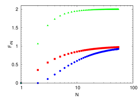
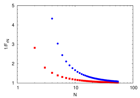
Figure 2: Left panel: Correction factors $F_{2{\scriptscriptstyle N}}={\left\langle n(n{-}1)\right\rangle}_{\!\!\scriptscriptstyle N}/{\left\langle n\right\rangle}_{\!\!\scriptscriptstyle N}^{2}$ (red squares) and $F_{3{\scriptscriptstyle N}}={\left\langle n(n{-}1)(n{-}2)\right\rangle}_{\!\!\scriptscriptstyle N}/{\left\langle n\right\rangle}_{\!\!\scriptscriptstyle N}^{3}$ (blue circles) as defined in Eq. (63) as well as $G_{3{\scriptscriptstyle N}}$ (green triangles) of Eq. (77), for the UA1 dataset used in Ref. [64]. Right panel: inverse factors as used in the normalisation of internal cumulants Eqs. (81)–(82) and (92)–(93).

It is of interest to zoom in on the approach to the poissonian limit of 1 and to compare these corrections to the equivalent charged-multiplicity-based ones, which for the case of fixed $N$, would be just $N(N{-}1)/N^{2}$ and $N(N{-}1)(N{-}2)/N^{3}$. In Fig. 3, the poissonian limit corresponds to zero on the $y$-axis. It is clear that the fixed-$N$ factors go some way to correct for the fixed-$N$ conditioning; the gap between them is approximately determined by ${\left\langle n^{{\underline{r}}}\right\rangle}_{\!\!\scriptscriptstyle N}/N^{{\underline{r}}}$, i.e. by the exact definition and outcome space for $n$.

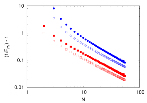
Figure 3: Comparison, for the same UA1 data and cuts, of $(1/F_{2{\scriptscriptstyle N}})-1$ (red filled squares), $(1/F_{3{\scriptscriptstyle N}})-1$ (blue filled circles), both averages over $n$ for fixed $N$, with prefactors $[N^{2}/N(N{-1})]-1$ (red open squares) and $[N^{3}/N(N{-1})(N{-}2)]-1$ (blue open circles). The poissonian limit is represented by zero on the $y$-axis, i.e. 100 times the $y$-scale represents the percentage deviation from the poissonian limit.

3.6 Eliminating fluctuations in ${n}$

We return briefly to the first choice in Section 3.2.3 i.e. $\alpha({\bm{p}}\,|\,{{\mathcal{S}}_{{n}{\scriptscriptstyle N}}})=\rho({\bm{p}}\,|\,{{\mathcal{S}}_{{n}{\scriptscriptstyle N}}})/n$ which would permit different physics for each $(N,{n})$ combination. If we were willing and able to do analyses for each ${{\mathcal{S}}_{{n}{\scriptscriptstyle N}}}$, we would use the fixed-$(N,n)$ equivalent of (75)–(3.3) derived from $\kappa^{\rm ref}({\bm{p}}_{1},\ldots,{\bm{p}}_{r}\,|\,{{\mathcal{S}}_{{n}{\scriptscriptstyle N}}})=(-1)^{r-1}\,(r-1)!\;{n}\prod_{k=1}^{r}\rho({\bm{p}}_{k}\,|\,{{\mathcal{S}}_{{n}{\scriptscriptstyle N}}})$,

$$\kappa^{I}({\bm{p}}_{1},{\bm{p}}_{2}\,|\,{{\mathcal{S}}_{{n}{\scriptscriptstyle N}}}) =\rho({\bm{p}}_{1},{\bm{p}}_{2}\,|\,{{\mathcal{S}}_{{n}{\scriptscriptstyle N}}})-\left(1-\tfrac{1}{n}\right)\rho({\bm{p}}_{1}\,|\,{{\mathcal{S}}_{{n}{\scriptscriptstyle N}}})\;\rho({\bm{p}}_{2}\,|\,{{\mathcal{S}}_{{n}{\scriptscriptstyle N}}})$$ (94)

$$\kappa^{I}({\bm{p}}_{1},{\bm{p}}_{2},{\bm{p}}_{3}\,|\,{{\mathcal{S}}_{{n}{\scriptscriptstyle N}}}) =\rho({\bm{p}}_{1},{\bm{p}}_{2},{\bm{p}}_{3}\,|\,{{\mathcal{S}}_{{n}{\scriptscriptstyle N}}})-[3]\,\rho({\bm{p}}_{1},{\bm{p}}_{2}\,|\,{{\mathcal{S}}_{{n}{\scriptscriptstyle N}}})\;\rho({\bm{p}}_{3}\,|\,{{\mathcal{S}}_{{n}{\scriptscriptstyle N}}})$$

$$\quad+2\left(1-\tfrac{1}{n^{2}}\right)\rho({\bm{p}}_{1}\,|\,{{\mathcal{S}}_{{n}{\scriptscriptstyle N}}})\;\rho({\bm{p}}_{2}\,|\,{{\mathcal{S}}_{{n}{\scriptscriptstyle N}}})\;\rho({\bm{p}}_{3}\,|\,{{\mathcal{S}}_{{n}{\scriptscriptstyle N}}})$$ (95)

and normalise by $\rho^{\rm ref}({\bm{p}}_{1},\ldots,{\bm{p}}_{r}\,|\,{{\mathcal{S}}_{{n}{\scriptscriptstyle N}}})=(n^{{\underline{r}}}/n^{r})\,\prod_{k=1}^{r}\rho({\bm{p}}_{k}\,|\,{{\mathcal{S}}_{{n}{\scriptscriptstyle N}}})$. Where that is not possible, we can still average over the above to form “Averaged Internal” (AI) correlations (see Section 5), but in this case averaging over $n$ for fixed $N$,

$$\kappa^{\rm\scriptscriptstyle SRC}({\bm{p}}_{1},{\bm{p}}_{2}\,|\,{{\mathcal{S}}_{\scriptscriptstyle N}}) ={\left\langle\kappa^{I}({\bm{p}}_{1},{\bm{p}}_{2}\,|\,{{\mathcal{S}}_{{n}{\scriptscriptstyle N}}})\right\rangle}_{\!\!\scriptscriptstyle N}$$ (96)

$$\kappa^{\rm\scriptscriptstyle SRC}({\bm{p}}_{1},{\bm{p}}_{2},{\bm{p}}_{3}\,|\,{{\mathcal{S}}_{\scriptscriptstyle N}}) ={\left\langle\kappa^{I}({\bm{p}}_{1},{\bm{p}}_{2},{\bm{p}}_{3}\,|\,{{\mathcal{S}}_{{n}{\scriptscriptstyle N}}})\right\rangle}_{\!\!\scriptscriptstyle N}$$ (97)

and normalise if necessary by the moment $\rho^{\rm\scriptscriptstyle SRC}({\bm{p}}_{1},\ldots,{\bm{p}}_{r}\,|\,{{\mathcal{S}}_{\scriptscriptstyle N}})={\left\langle(n^{{\underline{r}}}/n^{r})\,\prod_{k=1}^{r}\rho({\bm{p}}_{k}\,|\,{{\mathcal{S}}_{{n}{\scriptscriptstyle N}}})\right\rangle}_{\!\!\scriptscriptstyle N}$. Given that this involves products of moments in the subsubsample ${{\mathcal{S}}_{{n}{\scriptscriptstyle N}}}$, event mixing would have to be restricted to the same subsubsamples also; for example

$${\left\langle\left(1-\tfrac{1}{{n}}\right)\rho({\bm{p}}_{1}\,|\,{{\mathcal{S}}_{{n}{\scriptscriptstyle N}}})\,\rho({\bm{p}}_{2}\,|\,{{\mathcal{S}}_{{n}{\scriptscriptstyle N}}})\right\rangle}_{\!\!\scriptscriptstyle N} =\sum_{{n}=2}^{N}\frac{{{\mathcal{E}}_{{n}{\scriptscriptstyle N}}}}{{{\mathcal{E}}_{\scriptscriptstyle N}}}\left(1-\tfrac{1}{{n}}\right)\frac{1}{({{\mathcal{E}}_{{n}{\scriptscriptstyle N}}})^{2}}\sum_{a,b\,\in\,{{\mathcal{S}}_{{n}{\scriptscriptstyle N}}}}\hat{\rho}({\bm{p}}_{1}\,|\,{n},N,{\bm{P}}^{a})\,\hat{\rho}({\bm{p}}_{2}\,|\,{n},N,{\bm{P}}^{b})$$ (98)

The transformation to pair variables works in the same way as in previous sections.

4 Statistical errors

While the various versions of internal cumulants, constructed above may all be relevant at some point, we concentrate on finding expressions for experimental standard errors for the unnormalised and normalised internal cumulants of Eqs. (90)–(93). This turns out to be more subtle than merely applying a generic root-mean-square prescription. We shall show in this section that standard errors implemented thus far may have been underestimated even in the standard two-particle case.

The calculations performed in this section belong to the “frequentist” view of probability; a proper Bayesian analysis, which can be expected to rest on more solid foundations, is beyond the scope of this paper. The two viewpoints can reasonably be expected to yield similar results in the limit of large bin contents and sample sizes.

In this section, we often simplify notation by writing $\rho_{r}(Q\,|\,{{\mathcal{S}}_{\scriptscriptstyle N}})\to\rho_{\scriptscriptstyle rN}$ and $\rho_{1}{\otimes}\rho_{1}(Q\,|\,{{\mathcal{S}}_{\scriptscriptstyle N}})\to\rho_{\scriptscriptstyle 1N}^{2}$ etc, since the formulae apply to samples and variables of any kind.

4.1 Propagation of statistical errors

Because cumulants can be measured only through the moments that enter their definitions, the first task is to identify which moment variances and covariances are needed. By means of standard error propagation [68], we find the sample variances for second-order internal cumulants of Eqs. (90) and Eq. (92) to be

$$\mathrm{var}(\kappa_{2}^{I}(Q\,|\,{{\mathcal{S}}_{\scriptscriptstyle N}})) =\mathrm{var}(\rho_{\scriptscriptstyle 2N}-F_{2{\scriptscriptstyle N}}\,\rho_{\scriptscriptstyle 1N}^{2})=\mathrm{var}(\rho_{\scriptscriptstyle 2N})+F_{2{\scriptscriptstyle N}}^{2}\,\mathrm{var}(\rho_{\scriptscriptstyle 1N}^{2})-2\,F_{2{\scriptscriptstyle N}}\,\mathrm{cov}(\rho_{\scriptscriptstyle 2N},\rho_{\scriptscriptstyle 1N}^{2})$$ (99)

$$\mathrm{var}(K_{2}^{I}(Q\,|\,{{\mathcal{S}}_{\scriptscriptstyle N}})) =\mathrm{var}\left(\frac{1}{F_{2{\scriptscriptstyle N}}}\frac{\rho_{\scriptscriptstyle 2N}}{\rho_{\scriptscriptstyle 1N}^{2}}-1\right)$$ (100)

$$=\left[\frac{1}{F_{2{\scriptscriptstyle N}}}\frac{\rho_{\scriptscriptstyle 2N}}{\rho_{\scriptscriptstyle 1N}^{2}}\right]^{2}\left[\frac{\mathrm{var}(\rho_{\scriptscriptstyle 2N})}{\rho_{\scriptscriptstyle 2N}^{2}}+\frac{\mathrm{var}(\rho_{\scriptscriptstyle 1N}^{2})}{\rho_{\scriptscriptstyle 1N}^{4}}-2\frac{\mathrm{cov}(\rho_{\scriptscriptstyle 2N},\rho_{\scriptscriptstyle 1N}^{2})}{\rho_{\scriptscriptstyle 2N}\cdot\rho_{\scriptscriptstyle 1N}^{2}}\right]$$ (101)

under the assumption that $\mathrm{var}(F_{2{\scriptscriptstyle N}})$ is much smaller than the other variances, so that $F_{2{\scriptscriptstyle N}}$ can be treated as a constant; this is the case if there are many bins for $Q$. Similarly, from (3.3), the variance of the unnormalised internal cumulant is, assuming $G_{3}$ of Eq. (77) to be constant,

$$\mathrm{var}(\kappa_{3}^{I}({Q_{\scriptscriptstyle a}}\,|\,{{\mathcal{S}}_{\scriptscriptstyle N}})) =\mathrm{var}\left[\rho_{\scriptscriptstyle 3N}-3\,\rho_{\scriptscriptstyle 2N}\rho_{\scriptscriptstyle 1N}+G_{3}\,\rho_{\scriptscriptstyle 1N}^{3}\right]$$ (102)

$$=\mathrm{var}(\rho_{\scriptscriptstyle 3N})+9\,\mathrm{var}(\rho_{\scriptscriptstyle 2N}\rho_{\scriptscriptstyle 1N})+G_{3}^{2}\mathrm{var}(\rho_{\scriptscriptstyle 1N}^{3})$$

$$\quad-6\,\mathrm{cov}(\rho_{\scriptscriptstyle 3N},\rho_{\scriptscriptstyle 2N}\rho_{\scriptscriptstyle 1N})+2G_{3}\,\mathrm{cov}(\rho_{\scriptscriptstyle 3N},\rho_{\scriptscriptstyle 1N}^{3})-6G_{3}\,\mathrm{cov}(\rho_{\scriptscriptstyle 2N}\rho_{\scriptscriptstyle 1N},\rho_{\scriptscriptstyle 1N}^{3}),$$ (103)

while the normalised version has variance (again assuming $\mathrm{var}(G_{3})\ll\mathrm{var}\rho_{r}$)

$$\mathrm{var}(K_{3}^{I}({Q_{\scriptscriptstyle a}}\,|\,{{\mathcal{S}}_{\scriptscriptstyle N}})) =\mathrm{var}\left[\frac{\rho_{\scriptscriptstyle 3N}-3\rho_{\scriptscriptstyle 2N}\rho_{\scriptscriptstyle 1N}+G_{3}\rho_{\scriptscriptstyle 1N}^{3}}{F_{3{\scriptscriptstyle N}}\rho_{\scriptscriptstyle 1N}^{3}}\right]=\frac{1}{F_{3{\scriptscriptstyle N}}^{2}}\mathrm{var}\left[\frac{\rho_{\scriptscriptstyle 3N}-3\rho_{\scriptscriptstyle 2N}\rho_{\scriptscriptstyle 1N}}{\rho_{\scriptscriptstyle 1N}^{3}}+G_{3}\right]$$ (104)

$$=\left[\frac{\rho_{\scriptscriptstyle 3N}-3\rho_{\scriptscriptstyle 2N}\rho_{\scriptscriptstyle 1N}}{F_{3{\scriptscriptstyle N}}\,\rho_{\scriptscriptstyle 1N}^{3}}\right]^{2}\left[\frac{\mathrm{var}(\rho_{\scriptscriptstyle 3N}-3\rho_{\scriptscriptstyle 2N}\rho_{\scriptscriptstyle 1N})}{(\rho_{\scriptscriptstyle 3N}-3\rho_{\scriptscriptstyle 2N}\rho_{\scriptscriptstyle 1N})^{2}}+\frac{\mathrm{var}(\rho_{\scriptscriptstyle 1N}^{3})}{\rho_{\scriptscriptstyle 1N}^{6}}-\frac{2\mathrm{cov}(\rho_{\scriptscriptstyle 3N}-3\rho_{\scriptscriptstyle 2N}\rho_{\scriptscriptstyle 1N},\rho_{\scriptscriptstyle 1N}^{3})}{(\rho_{\scriptscriptstyle 3N}-3\rho_{\scriptscriptstyle 2N}\rho_{\scriptscriptstyle 1N})\rho_{\scriptscriptstyle 1N}^{3}}\right]$$

$$=\left[\frac{\rho_{\scriptscriptstyle 3N}-3\rho_{\scriptscriptstyle 2N}\rho_{\scriptscriptstyle 1N}}{F_{3{\scriptscriptstyle N}}\,\rho_{\scriptscriptstyle 1N}^{3}}\right]^{2}\biggl{[}\frac{\mathrm{var}(\rho_{\scriptscriptstyle 3N})+9\mathrm{var}(\rho_{\scriptscriptstyle 2N}\rho_{\scriptscriptstyle 1N})-6\mathrm{cov}(\rho_{\scriptscriptstyle 3N},\rho_{\scriptscriptstyle 2N}\rho_{\scriptscriptstyle 1N})}{(\rho_{\scriptscriptstyle 3N}-3\rho_{\scriptscriptstyle 2N}\rho_{\scriptscriptstyle 1N})^{2}}+\frac{\mathrm{var}(\rho_{\scriptscriptstyle 1N}^{3})}{\rho_{\scriptscriptstyle 1N}^{6}}$$

$$\hskip 96.0pt+\frac{6\mathrm{cov}(\rho_{\scriptscriptstyle 2N}\rho_{\scriptscriptstyle 1N},\rho_{\scriptscriptstyle 1N}^{3})-2\mathrm{cov}(\rho_{\scriptscriptstyle 3N},\rho_{\scriptscriptstyle 1N}^{3})}{(\rho_{\scriptscriptstyle 3N}-3\rho_{\scriptscriptstyle 2N}\rho_{\scriptscriptstyle 1N})\rho_{\scriptscriptstyle 1N}^{3}}\biggr{]}.$$ (105)

The unnormalised cumulants (90)–(91) and their variances (99) and (103) require knowledge of the multiplicity factorial moments $F_{2{\scriptscriptstyle N}},F_{3{\scriptscriptstyle N}}$, so that the individual terms must be accumulated until the entire sample has been analysed. By contrast, the normalised cumulants (92)–(93) and their variances (101) and (4.1) contain the multiplicity moments only as prefactors.

4.2 Expectation values of counters

While we shall not make direct use of the results in this section, it is nevertheless useful briefly to consider what we might mean by an “expectation value of experimental counters and densities”. For any scalar function $f({\bm{p}})$ of the momenta, the theoretical expectation value $E[f]$ is defined as the integral over the entire outcome space $\Omega$ of $f$ weighted by a “parent distribution” $P({\bm{p}})$, an abstract entity supposedly containing everything there is to know on this level,

$$E[f({\bm{p}})]=\int_{\Omega}d{\bm{p}}\,P({\bm{p}})\,f({\bm{p}}).$$ (106)

Purely theoretical concepts such as $P({\bm{p}})$ and $E[f]$ should be given little or no room in a strongly experimentally-oriented study. In calculating standard errors on counters below, we shall, however, make use of the exact factorisation that expectation values provide whenever two variables $x,y$ are statistically independent, $E[xy]=\int dx\,dy\,P(x,y)\,xy=E[x]\,E[y]$.

Expectation values for pairwise variables such as the four-momentum difference $Q$ we are considering here must be based on the underlying physics. We can deduce some properties of the parent distribution based on the usual definition of the femtoscopic correlation function

$$C_{2}(Q) \equiv K_{2}(Q)+1=\frac{\rho_{2}^{\rm sibling}(Q)}{\rho_{2}^{\rm reference}(Q)}=\frac{{\bigl{\langle}\hat{\rho}(Q^{aa})\bigr{\rangle}}}{{\bigl{\langle}{\bigl{\langle}\hat{\rho}(Q^{ab})\bigr{\rangle}}\bigr{\rangle}}}$$ (107)

is a function of two entirely different quantities: the four-momentum differences $Q^{aa}$ of “sibling” tracks taken from the same event $a$ and one constructed from the mixed-event sample using tracks from different events, written as $Q^{ab}$, $Q^{bc}$ etc. For second-order correlations, the parent distribution is therefore necessarily a two-variable probability $P(Q^{aa},Q^{bc})$ which, depending on whether the cases $b{=}a$ and $c{=}a$ occur, may or may not factorise into a “sibling” and a “mixed” marginal probability

$$P(Q^{aa},Q^{bc}) =P_{s}(Q^{aa})\;P_{m}(Q^{bc})\quad\text{iff }a{\neq}b{\neq}c,$$ (108)

but (unless $a{=}b{=}c$) the marginals will always be

$$P_{s}(Q^{aa}) =\int dQ^{bc}\,P(Q^{aa},Q^{bc}),$$ (109)

$$P_{m}(Q^{bc}) =\int dQ^{aa}\,P(Q^{aa},Q^{bc}).$$ (110)

The shapes of $P_{s}(Q)$ and $P_{m}(Q)$ must necessarily be different since it is precisely this difference that leads to a nontrivial signal in (107). In terms of this joint probability, we can write expectation values of eventwise counters (separately for inclusive, fixed-$N$ or fixed-$n$ cases) as

$$E[\hat{\rho}(Q^{aa})] =\int_{\Omega}dQ^{aa}dQ^{bc}\;P(Q^{aa},Q^{bc})\,\hat{\rho}_{aa}=\sum_{i\neq j}\int_{\Omega}dQ^{aa}\;P_{s}(Q^{aa})\,\delta(Q^{aa}-Q_{ij}^{aa})=\sum_{i\neq j}P_{s}(Q_{ij}^{aa}),$$ (111)

$$E[\hat{\rho}(Q^{bc})] =\int_{\Omega}dQ^{aa}dQ^{bc}\;P(Q^{aa},Q^{bc})\,\hat{\rho}_{bc}=\sum_{i,j}\int_{\Omega}dQ^{bc}\;P_{m}(Q^{bc})\,\delta(Q^{bc}-Q_{ij}^{bc})=\sum_{i,j}P_{m}(Q_{ij}^{bc}).$$ (112)

Later, we shall meet expectation values for cases such as $a{=}c$,

$$E[\hat{\rho}(Q^{aa})\,\hat{\rho}(Q^{ab})] =\sum_{i\neq j}\sum_{k,\ell}\int_{\Omega}dQ^{aa}\,dQ^{ab}\;P(Q^{aa},Q^{ab})\;\delta(Q^{aa}-Q_{ij}^{aa})\delta(Q^{ab}-Q_{k\ell}^{ab})$$

$$=\sum_{i\neq j}\sum_{k,\ell}P(Q_{ij}^{aa},Q_{k\ell}^{ab})$$ (113)

which definitely does not factorise. The above expressions can be simplified because we know that the parent distribution is not a function of the individual track indices $i,j,k,\ell$

$$P(Q_{ij}^{aa},Q_{k\ell}^{bc}) =P(Q^{aa},Q^{bc})\qquad\forall\;i,j,k,\ell$$ (114)

and similarly $P_{s}(Q_{ij}^{aa})=P_{s}(Q^{aa})$ and $P_{m}(Q_{k\ell}^{bc})=P_{m}(Q^{bc})$. For the event-averaged counters, this results in

$$E[\rho_{aa}(Q)] ={\left\langle n_{a}^{{\underline{2}}}\right\rangle}_{\!\!\scriptscriptstyle N}P_{s}(Q^{aa})$$ (115)

$$E[\rho_{bc}(Q)] ={\left\langle n_{b}\right\rangle}_{\!\!\scriptscriptstyle N}{\left\langle n_{c}\right\rangle}_{\!\!\scriptscriptstyle N}P_{m}(Q^{bc})$$ (116)

or in terms of the notation of Section 3.4,

$$E[\rho_{\scriptscriptstyle 2N}(Q)] ={\left\langle n^{{\underline{2}}}\right\rangle}_{\!\!\scriptscriptstyle N}P_{s}(Q^{aa})$$ (117)

$$E[\rho_{\scriptscriptstyle 1N}{\otimes}\rho_{\scriptscriptstyle 1N}(Q)] ={\left\langle n\right\rangle}_{\!\!\scriptscriptstyle N}^{2}P_{m}(Q^{bc}).$$ (118)

As mentioned, we do not need the factorisation (108) of $P(Q^{aa},Q^{bc})$ as long as we keep careful track of the equal-event-indices cases. Whenever $a{\neq}b$ or $a{\neq}c$, independence of the events ensures that expectation values of products of any functions $f(Q^{aa})$ and $g(Q^{ab})$ of the pair variables do factorise,

$$E[f(Q^{aa})\,g(Q^{ab})] =E[f(Q^{aa})]\,E[g(Q^{ab})]\qquad a\neq b$$ (119)

For third-order correlations, the parent distribution is a function of three different variables $Q^{aaa}$, $Q^{bbc}$ and $Q^{def}$ containing respectively three, two or one track from the same event and corresponding considerations regarding equal and unequal event indices apply there, too.

4.3 Statistical error calculation from first principles

It was shown in Section 4.2 that expectation values would have well-defined meanings in terms of underlying parent distributions and their marginals if their parent distributions were known, which, however, they are not. We are therefore forced to revert from expectation values $E[\cdot]$ to sample averages $\langle\cdot\rangle$ after completing a calculation. The real use of such expectation values in frequentist statistics has been in the form of a gedankenexperiment which we now reproduce from Kendall [68]. Let $x$ be any generic eventwise counter or any other eventwise statistic. Since the formulae in this section remain true for inclusive and fixed-$N$ samples, we omit any notation related to $N$ in this derivation. In this simplified notation, the well-known standard error of the sample mean ${\bigl{\langle}x\bigr{\rangle}}$ is given by (simplifying ${{\mathcal{E}}}-1\to{{\mathcal{E}}}$)

$$\sigma({\bigl{\langle}x\bigr{\rangle}}) =\sqrt{\mathrm{var}({\bigl{\langle}x\bigr{\rangle}})}\ =\ \sqrt{\tfrac{1}{{{\mathcal{E}}}}{\left[{\bigl{\langle}x^{2}\bigr{\rangle}}-{\bigl{\langle}x\bigr{\rangle}}^{2}\right]}}$$ (120)

which follows from the combinatorics of equal and unequal event indices by the above artificial use of expectation values, reverting from expectation values $E[\cdot]$ to sample means ${\bigl{\langle}\cdot\bigr{\rangle}}$ in the last step:

$$\mathrm{var}({\bigl{\langle}x\bigr{\rangle}}) =E[{\bigl{\langle}x\bigr{\rangle}}^{2}]-E[{\bigl{\langle}x\bigr{\rangle}}]^{2}=\frac{1}{{{\mathcal{E}}}^{2}}\sum_{a,b}\Bigl{[}E[x_{a}x_{b}]-E[x_{a}]\,E[x_{b}]\Bigr{]}$$ (121)

$$=\frac{1}{{{\mathcal{E}}}^{2}}\sum_{a=b}\Bigl{[}E[x_{a}x_{b}]-E[x_{a}]\,E[x_{b}]\Bigr{]}+\frac{1}{{{\mathcal{E}}}^{2}}\sum_{a\neq b}\Bigl{[}E[x_{a}]\,E[x_{b}]-E[x_{a}]\,E[x_{b}]\Bigr{]}$$

$$=\frac{1}{{{\mathcal{E}}}^{2}}\sum_{a}\Bigl{[}E[x^{2}]-E[x]^{2}\Bigr{]}+0=\frac{1}{{{\mathcal{E}}}}\Bigl{[}{\bigl{\langle}x^{2}\bigr{\rangle}}-{\bigl{\langle}x\bigr{\rangle}}^{2}\Bigr{]},$$ (122)

where we have used the fact that $E[x_{a}x_{b}]=E[x_{a}]\,E[x_{b}]\;\forall a{\neq}b$ and assumed that all $x$ are identically distributed, $E[x_{a}]=E[x]\;\forall a$. Equality or inequality of event indices is thus crucial. We shall follow the same approach below, keeping careful track of equal and unequal event indices, factorising expectation values for unequal event indices, and reverting to sample means in the last step.

4.4 Variances and covariances for multiple event averages

4.4.1 Statistical errors for second-order cumulants

According to Eqs. (99)–(4.1), we must handle variances and covariances of products of several event averages. To derive these, we shall use the following shortened notation: Letting $\delta_{ij}^{ab}\equiv\delta(Q-Q_{ij}^{ab})$ etc, then $\hat{\rho}_{aa}=\sum_{i\neq j}\delta(Q-Q_{ij}^{aa})=\sum_{i\neq j}\delta_{ij}^{aa}$ is the eventwise pair counter for event $a$, while $\hat{\rho}_{bc}=\sum_{i,j}\delta(Q-Q_{ij}^{bc})=\sum_{i,j}\delta_{ij}^{bc}$ is the mixed-event counter of events $b$ and $c$ (with $b{\neq}c{\neq}a$ assumed), so that $\rho_{2}(Q)={\bigl{\langle}\hat{\rho}_{aa}\bigr{\rangle}_{\!a}}$ while $\rho_{1}{\otimes}\rho_{1}(Q)={\bigl{\langle}\hat{\rho}_{ab}\bigr{\rangle}_{\!ab}}$ is a double event average. We reserve the event index $a$ for the “sibling” event whose correlations are currently being analysed, and use indices $b,c,\ldots,t,u,v,w,\ldots$ for events entering the event-mixing parts. All quantities are assumed to be measured within a particular subsample ${{\mathcal{S}}_{\scriptscriptstyle N}}$ but we omit the $N$-subscript and the argument. The event-index subscripts such as $\langle\cdot\rangle_{bc}$ above are included or omitted depending on whether they convey relevant information on the specific averaging.

In this notation, the method that led to Eq. (122) reads

$$\mathrm{var}(\rho_{2}) =\mathrm{var}({\bigl{\langle}\hat{\rho}_{aa}\bigr{\rangle}_{\!a}})=\frac{1}{{{\mathcal{E}}}^{2}}\sum_{a,b}\Bigl{[}E(\hat{\rho}_{aa}\hat{\rho}_{bb})-E(\hat{\rho}_{aa})\,E(\hat{\rho}_{bb})\Bigr{]}=\frac{1}{{{\mathcal{E}}}}\Bigl{[}{\bigl{\langle}(\hat{\rho}_{aa})^{2}\bigr{\rangle}}-{\bigl{\langle}\hat{\rho}_{aa}\bigr{\rangle}}^{2}\Bigr{]}.$$ (123)

The same method of disentangling the combinatorics of equal and unequal event indices is applied consistently to all variances and covariances below. The $\rho_{1}^{2}$-term in second-order cumulants has variance

$$\mathrm{var}(\rho_{1}{\otimes}\rho_{1}) =\mathrm{var}({\bigl{\langle}\hat{\rho}_{bc}\bigr{\rangle}_{\!bc}})=\frac{1}{({{\mathcal{E}}}^{{\underline{2}}})^{2}}\sum_{b\neq c}\sum_{d\neq e}\Bigl{[}E(\hat{\rho}_{bc}\hat{\rho}_{de})-E(\hat{\rho}_{bc})\,E(\hat{\rho}_{de})\Bigr{]}.$$ (124)

The case $b{\neq}c{\neq}d{\neq}e$ yields zero, but the cases $b{=}d{\neq}c{\neq}e$ and three other equivalent combinations yield

$$\mathrm{var}(\rho_{1}{\otimes}\rho_{1}) =\frac{4{{\mathcal{E}}}^{\underline{3}}}{({{\mathcal{E}}}^{{\underline{2}}})^{2}}\Bigl{[}E[\hat{\rho}_{bc}\hat{\rho}_{be}]-E[\hat{\rho}_{bc}]\,E[\hat{\rho}_{be}]\Bigr{]}$$

$$\to\ \frac{4{{\mathcal{E}}}^{\underline{3}}}{({{\mathcal{E}}}^{{\underline{2}}})^{2}}\Bigl{[}{\bigl{\langle}\hat{\rho}_{bc}\hat{\rho}_{be}\bigr{\rangle}_{\!bce}}-{\bigl{\langle}\hat{\rho}_{bc}\bigr{\rangle}}\,{\bigl{\langle}\hat{\rho}_{be}\bigr{\rangle}}\Bigr{]}\quad\to\quad\frac{4}{{{\mathcal{E}}}}\Bigl{[}{\bigl{\langle}\hat{\rho}_{bc}\hat{\rho}_{be}\bigr{\rangle}}-(\rho_{1}{\otimes}\rho_{1})^{2}\Bigr{]}$$ (125)

where in the second step we reverted $E[\,]\to{\bigl{\langle}\,\bigr{\rangle}}$ and in the third assumed ${{\mathcal{E}}}\gg 1$. Note that the requirement $b{\neq}c{\neq}e$ implies that ${\bigl{\langle}\hat{\rho}_{bc}\hat{\rho}_{be}\bigr{\rangle}_{\!bce}}={\bigl{\langle}{\bigl{\langle}\sum_{i\neq j}\delta_{ij}^{bc}\bigr{\rangle}_{\!c}}{\bigl{\langle}\sum_{k\neq l}\delta_{k\ell}^{be}\bigr{\rangle}_{\!e}}\bigr{\rangle}_{\!b}}$ cannot be simplified to the square of a single counter ${\bigl{\langle}\bigl{\langle}\sum_{i\neq j}\delta_{ij}^{bc}\bigr{\rangle}_{c}^{2}\bigr{\rangle}_{\!b}}$: the event mixing involves three different events, not two. Secondly, the combinations of two equalities $b{=}d{\neq}c{=}e$ and $b{=}e{\neq}c{=}d$ in (124) yield another term of order ${{\mathcal{E}}}^{-2}$,

$$\frac{2}{{{\mathcal{E}}}^{\underline{2}}}\Bigl{[}{\bigl{\langle}\hat{\rho}_{bd}\hat{\rho}_{bd}\bigr{\rangle}_{\!bd}}-(\rho_{1}{\otimes}\rho_{1})^{2}\Bigr{]}$$ (126)

which we can safely neglect when ${\bigl{\langle}{n}^{2}\bigr{\rangle}}/{{\mathcal{E}}}\ll 1$ except when there are few bins or large multiplicities even in small bins. It is worth emphasising that the extra factor 4 which appears in Eq. (4.4.1) arises from the same method that has been used for decades to justify use of Eq. (120). We find, by the same method, that the covariance between $\rho_{2}$ and $\rho_{1}{\otimes}\rho_{1}$ is given by

$$\mathrm{cov}(\rho_{2},\rho_{1}{\otimes}\rho_{1}) =\mathrm{cov}({\bigl{\langle}\hat{\rho}_{dd}\bigr{\rangle}},{\bigl{\langle}\hat{\rho}_{bc}\bigr{\rangle}})=\frac{1}{{{\mathcal{E}}}\,{{\mathcal{E}}}^{{\underline{2}}}}\sum_{d}\sum_{b\neq c}\Bigl{[}E(\hat{\rho}_{dd}\hat{\rho}_{bc})-E(\hat{\rho}_{dd})\,E(\hat{\rho}_{bc})\Bigr{]}$$ (127)

$$=\frac{2}{{{\mathcal{E}}}}\Bigl{[}{\bigl{\langle}\hat{\rho}_{dd}\hat{\rho}_{db}\bigr{\rangle}}-{\bigl{\langle}\hat{\rho}_{dd}\bigr{\rangle}}{\bigl{\langle}\hat{\rho}_{dc}\bigr{\rangle}}\Bigr{]}=\frac{2}{{{\mathcal{E}}}}\Bigl{[}{\bigl{\langle}\hat{\rho}_{dd}\hat{\rho}_{dc}\bigr{\rangle}}-(\rho_{2})(\rho_{1}{\otimes}\rho_{1})\Bigr{]}$$ (128)

so that we must in addition accumulate, for every event $d$, the product of the counters

$$\hat{\rho}_{dd}\hat{\rho}_{dc}=\sum_{i\neq j}\delta_{ij}^{dd}\sum_{k}\Bigl{\langle}\sum_{\ell}\delta_{k\ell}^{dc}\Bigr{\rangle}_{c}.$$ (129)

Note that there is no restriction on track indices $k{\neq}i$ or $k{\neq}j$ in the $d$-event, meaning that events with $n(a)=2$ contribute to this counter which would otherwise not be the case. Combining these, we find, to leading order in ${{\mathcal{E}}}^{-1}$ and renaming mixed-event indices,

$$\mathrm{var}(\kappa_{2}^{I}) =\frac{1}{{{\mathcal{E}}}}\left\{{\bigl{\langle}\left(\hat{\rho}_{aa}-2F_{2{\scriptscriptstyle N}}\hat{\rho}_{ac}\right)\left(\hat{\rho}_{aa}-2F_{2{\scriptscriptstyle N}}\hat{\rho}_{ad}\right)\bigr{\rangle}}_{a}-\left(\rho_{2}-2F_{2{\scriptscriptstyle N}}\,\rho_{1}{\otimes}\rho_{1}\right)^{2}\right\}$$ (130)

with all event indices strictly unequal and $c$- and $d$-event averages understood where appropriate. Contrasting this with the traditional way to calculate the same variance,

$$\mathrm{var}(\kappa_{2}^{I}) =\frac{1}{{{\mathcal{E}}}}\left\{{\bigl{\langle}\left(\hat{\rho}_{aa}-F_{2{\scriptscriptstyle N}}\hat{\rho}_{ac}\right)\left(\hat{\rho}_{aa}-F_{2{\scriptscriptstyle N}}\hat{\rho}_{ad}\right)\bigr{\rangle}}-\left(\rho_{2}-F_{2{\scriptscriptstyle N}}\,\rho_{1}{\otimes}\rho_{1}\right)^{2}\right\}$$ (131)

it is clear that in previous analyses the two possible ways to set $a$ equal to $b$ or $c$ were overlooked, while normal (non-internal) cumulants also omit the $F_{2{\scriptscriptstyle N}}$.

4.4.2 Statistical errors for third-order cumulants

In third order, we shall need $\delta_{ijk}^{abc}\equiv\delta({Q_{\scriptscriptstyle a}}-Q_{ijk}^{abc})$ and similar quantities, and the notation for counters $\hat{\rho}_{aaa}$, $\hat{\rho}_{aab}$ and $\hat{\rho}_{abc}$ corresponding to the event averages $\rho_{3}({Q_{\scriptscriptstyle a}})={\bigl{\langle}\hat{\rho}_{aaa}\bigr{\rangle}}$, $\rho_{2}{\otimes}\rho_{1}({Q_{\scriptscriptstyle a}})={\bigl{\langle}\hat{\rho}_{aab}\bigr{\rangle}}$ and $\rho_{1}{\otimes}\rho_{1}{\otimes}\rho_{1}({Q_{\scriptscriptstyle a}})={\bigl{\langle}\hat{\rho}_{abc}\bigr{\rangle}}$ respectively. Clearly, $a{\neq}b{\neq}c$ must hold in the third order case. We obtain for the necessary third-order quantities (shuffling and/or renaming indices if necessary)

$$\mathrm{var}(\rho_{3}) =\frac{1}{{{\mathcal{E}}}}\Bigl{[}{\bigl{\langle}(\hat{\rho}_{aaa})^{2}\bigr{\rangle}_{\!a}}-\rho_{3}^{2}\Bigr{]}$$ (132)

$$\mathrm{cov}(\rho_{3},\rho_{2}{\otimes}\rho_{1}) =\frac{1}{{{\mathcal{E}}}\,{{\mathcal{E}}}^{{\underline{2}}}}\sum_{r}\sum_{s\neq t}\Bigl{[}E(\hat{\rho}_{rrr}\hat{\rho}_{sst})-E(\hat{\rho}_{rrr})\,E(\hat{\rho}_{sst})\Bigr{]}$$

$$=\frac{1}{{{\mathcal{E}}}}\Bigl{[}{\bigl{\langle}\hat{\rho}_{rrr}\hat{\rho}_{rrs}\bigr{\rangle}}+{\bigl{\langle}\hat{\rho}_{rrr}\hat{\rho}_{rss}\bigr{\rangle}}-2\rho_{3}(\rho_{2}{\otimes}\rho_{1})\Bigr{]}$$ (133)

with $\hat{\rho}_{rrr}\hat{\rho}_{rrs}=\sum_{i\neq j\neq k}\delta_{ijk}^{rrr}\sum_{\ell\neq m}\Bigl{\langle}\sum_{n}\delta_{\ell mn}^{rrs}\Bigr{\rangle}_{s}$ and $\hat{\rho}_{rrr}\hat{\rho}_{rss}=\sum_{i\neq j\neq k}\delta_{ijk}^{rrr}\sum_{\ell}\Bigl{\langle}\sum_{m\neq n}\delta_{\ell mn}^{rss}\Bigr{\rangle}_{s}$. The remaining variances and covariances needed for third-order correlations with GHP topology are, after renaming of indices,

$$\mathrm{var}(\rho_{2}{\otimes}\rho_{1}) =\frac{{{\mathcal{E}}}^{{\underline{3}}}}{({{\mathcal{E}}}^{{\underline{2}}})^{2}}\sum_{g\neq e}\sum_{c\neq d}\Bigl{[}E(\hat{\rho}_{gge}\hat{\rho}_{ccd})-E(\hat{\rho}_{gge})\,E(\hat{\rho}_{ccd})\Bigr{]}$$

$$=\frac{{{\mathcal{E}}}^{{\underline{3}}}}{({{\mathcal{E}}}^{{\underline{2}}})^{2}}\Bigl{[}{\bigl{\langle}\hat{\rho}_{ggd}[\hat{\rho}_{ggc}+\hat{\rho}_{gcc}+\hat{\rho}_{ddc}+\hat{\rho}_{dcc}]\bigr{\rangle}}-4(\rho_{2}{\otimes}\rho_{1})^{2}\Bigr{]},$$ (134)

while we neglect

$$\frac{1}{{{\mathcal{E}}}^{\underline{2}}}\Bigl{[}\hat{\rho}_{ggc}\hat{\rho}_{ggc}+\hat{\rho}_{ggc}\hat{\rho}_{gcc}-2(\rho_{2}{\otimes}\rho_{1})^{2}\Bigr{]}.$$ (135)

The next term is simpler,

$$\mathrm{cov}(\rho_{3},\rho_{1}^{3}) =\frac{1}{{{\mathcal{E}}}\,{{\mathcal{E}}}^{{\underline{3}}}}\sum_{t}\sum_{u\neq v\neq w}\Bigl{[}E(\hat{\rho}_{ttt}\hat{\rho}_{uvw})-E(\hat{\rho}_{ttt})\,E(\hat{\rho}_{uvw})\Bigr{]}=\frac{3}{{{\mathcal{E}}}}\Bigl{[}{\bigl{\langle}\hat{\rho}_{ttt}\hat{\rho}_{tuv}\bigr{\rangle}}-\rho_{3}\rho_{1}^{3}\Bigr{]},$$ (136)

but the following is not,

$$\mathrm{cov}(\rho_{2}{\otimes}\rho_{1},\rho_{1}^{3}) =\frac{1}{{{\mathcal{E}}}^{{\underline{2}}}{{\mathcal{E}}}^{{\underline{3}}}}\sum_{u\neq v}\sum_{x\neq y\neq z}\Bigl{[}E(\hat{\rho}_{uuv}\hat{\rho}_{xyz})-E(\hat{\rho}_{uuv})\,E(\hat{\rho}_{xyz})\Bigr{]}$$ (137)

$$=\frac{3{{\mathcal{E}}}^{{\underline{4}}}}{{{\mathcal{E}}}^{{\underline{2}}}{{\mathcal{E}}}^{{\underline{3}}}}\Bigl{[}{\bigl{\langle}\hat{\rho}_{wwx}\hat{\rho}_{wyz}\bigr{\rangle}}+{\bigl{\langle}\hat{\rho}_{wxx}\hat{\rho}_{wyz}\bigr{\rangle}}-2(\rho_{2}\rho_{1})(\rho_{1}^{3})\Bigr{]}+\frac{6}{{{\mathcal{E}}}^{{\underline{2}}}}\Bigl{[}{\bigl{\langle}\hat{\rho}_{wwx}\hat{\rho}_{wxy}\bigr{\rangle}}-(\rho_{2}\rho_{1})(\rho_{1}^{3})\Bigr{]},$$ (138)

and the large number of combinations makes the variance of $\rho_{1}^{3}$ particularly complicated,

$$\mathrm{var}(\rho_{1}{\otimes}\rho_{1}{\otimes}\rho_{1}) =\frac{1}{({{\mathcal{E}}}^{{\underline{3}}})^{2}}\sum_{d\neq e\neq h}\sum_{b\neq p\neq q}\Bigl{[}E(\hat{\rho}_{deh}\hat{\rho}_{bpq})-E(\hat{\rho}_{deh})\,E(\hat{\rho}_{bpq})\Bigr{]}$$ (139)

$$=\frac{9{{\mathcal{E}}}^{{\underline{5}}}}{({{\mathcal{E}}}^{{\underline{3}}})^{2}}\Bigl{[}{\bigl{\langle}\hat{\rho}_{beh}\hat{\rho}_{bpq}\bigr{\rangle}_{\!}}-(\rho_{1}^{3})(\rho_{1}^{3})\Bigr{]}+\frac{18{{\mathcal{E}}}^{{\underline{4}}}}{({{\mathcal{E}}}^{{\underline{3}}})^{2}}\Bigl{[}{\bigl{\langle}\hat{\rho}_{beh}\hat{\rho}_{beq}\bigr{\rangle}_{\!}}-(\rho_{1}^{3})(\rho_{1}^{3})\Bigr{]}$$

$$+\frac{6}{{{\mathcal{E}}}^{{\underline{3}}}}\Bigl{[}{\bigl{\langle}\hat{\rho}_{beh}\hat{\rho}_{beh}\bigr{\rangle}_{\!}}-(\rho_{1}^{3})(\rho_{1}^{3})\Bigr{]}.$$ (140)

For large ${{\mathcal{E}}}$, the leading order terms will usually dominate, so that we can neglect the subleading terms. To leading order, we therefore obtain after substitution in (102) and again omitting brackets for non-$a$ event averages

$$\mathrm{var}(\kappa_{3}^{I}) =\frac{1}{{{\mathcal{E}}}}\biggl{\{}\biggl{\langle}\hat{\rho}_{aaa}^{2}+9\hat{\rho}_{aab}(\hat{\rho}_{aac}+\hat{\rho}_{acc}+\hat{\rho}_{bbc}+\hat{\rho}_{bcc})+9G_{3}^{2}\hat{\rho}_{aaa}(\hat{\rho}_{abc}\hat{\rho}_{ade})$$ (141)

$$\qquad\qquad-6\hat{\rho}_{aaa}(\hat{\rho}_{aab}+\hat{\rho}_{abb})+6G_{3}\hat{\rho}_{aaa}\hat{\rho}_{abc}-18G_{3}\hat{\rho}_{aab}(\hat{\rho}_{acd}+\hat{\rho}_{bcd})\biggr{\rangle}_{\!\!a}$$

$$\qquad-\biggl{[}\rho_{3}^{2}+36(\rho_{2}{\otimes}\rho_{1})^{2}+9G_{3}^{2}\,(\rho_{1}^{3})^{2}-12\rho_{3}(\rho_{2}{\otimes}\rho_{1})+6G_{3}\,\rho_{3}(\rho_{1})^{3}-36G_{3}^{2}(\rho_{2}{\otimes}\rho_{1})(\rho_{1})^{3}\biggr{]}\biggr{\}}$$

$$=\frac{1}{{{\mathcal{E}}}}\biggl{\{}\biggl{\langle}(\hat{\rho}_{aaa}-3\hat{\rho}_{aab}-3\hat{\rho}_{abb}+3G_{3}\hat{\rho}_{abc})(\hat{\rho}_{aaa}-3\hat{\rho}_{aad}-3\hat{\rho}_{add}+3G_{3}\hat{\rho}_{ade})\biggr{\rangle}_{\!\!a}$$

$$\qquad-\biggl{[}\rho_{3}-6\rho_{2}{\otimes}\rho_{1}+3G_{3}(\rho_{1})^{3}\biggr{]}^{2}\biggr{\}}.$$ (142)

While the factorised form is again instructive, it cannot be calculated in this form within the $a$-loop in the analysis since the $G_{3{\scriptscriptstyle N}}$ constants are known only on completion of the entire sample analysis. Rather, the full palette of product counters $\hat{\rho}\hat{\rho}$ has to be accumulated and averaged and combined only in the final phase of the analysis.

5 Averaged internal cumulants

As $N$ is only an approximation for the true total event multiplicity anyway, and for cases of small sample statistics, it may be necessary or desirable to group subsamples of fixed $N$ into multiplicity classes $N\in[A,B]$. It is important, however, not to simply lump all events within this multiplicity class into a single “half-inclusive” subsample, because, as has long been known [15], that results in terms entering the cumulants which arise solely to “multiplicity mixing” (MM) of events of different $N$. Given the arbitrary choice of $[A,B]$, such MM correlations are spurious and avoided in favour of “Averaged-Internal” (AI) correlations defined as follows. Using the renormalised multiplicity distribution

$${{\mathcal{R}}_{\scriptscriptstyle N}^{\prime}}=\frac{{{\mathcal{R}}_{\scriptscriptstyle N}}}{\sum_{N=A}^{B}{{\mathcal{R}}_{\scriptscriptstyle N}}}=\frac{{{\mathcal{E}}_{\scriptscriptstyle N}}}{\sum_{N=A}^{B}{{\mathcal{E}}_{\scriptscriptstyle N}}}$$ (143)

the AI unnormalised cumulants, reference distributions and normalised AI cumulants are

$$\kappa_{2}^{AI}(Q\,|\,{{\mathcal{S}}_{AB}}) =\sum_{N=A}^{B}{{\mathcal{R}}_{\scriptscriptstyle N}^{\prime}}\;\kappa_{2}^{I}(Q\,|\,{{\mathcal{S}}_{\scriptscriptstyle N}}),$$ (144)

$$\rho_{1}{\otimes}\rho_{1}(Q\,|\,{{\mathcal{S}}_{AB}}) =\sum_{N=A}^{B}{{\mathcal{R}}_{\scriptscriptstyle N}^{\prime}}\;F_{2{\scriptscriptstyle N}}\;\rho_{1}{\otimes}\rho_{1}(Q\,|\,{{\mathcal{S}}_{\scriptscriptstyle N}}),$$ (145)

$$K_{2}^{AI}(Q\,|\,{{\mathcal{S}}_{AB}}) =\frac{\kappa_{2}^{AI}(Q\,|\,{{\mathcal{S}}_{AB}})}{\rho_{1}{\otimes}\rho_{1}(Q\,|\,{{\mathcal{S}}_{AB}})}\ =\ \frac{\sum_{N=A}^{B}{{\mathcal{R}}_{\scriptscriptstyle N}^{\prime}}\,\rho_{2}(Q\,|\,{{\mathcal{S}}_{\scriptscriptstyle N}})}{\sum_{N=A}^{B}{{\mathcal{R}}_{\scriptscriptstyle N}^{\prime}}\,F_{2{\scriptscriptstyle N}}\,\rho_{1}{\otimes}\rho_{1}(Q\,|\,{{\mathcal{S}}_{\scriptscriptstyle N}})}\ -\ 1.$$ (146)

Note that the correction factors $F_{2{\scriptscriptstyle N}}$, which are normalised factorial moments of $n$ for fixed $N$, are part of the summed normalisations. In third order, we have correspondingly

$$\kappa_{3}^{AI}({Q_{\scriptscriptstyle a}}\,|\,{{\mathcal{S}}_{AB}}) =\sum_{N=A}^{B}{{\mathcal{R}}_{\scriptscriptstyle N}^{\prime}}\;\kappa_{3}^{I}({Q_{\scriptscriptstyle a}}\,|\,{{\mathcal{S}}_{\scriptscriptstyle N}}),$$ (147)

$$\rho_{1}{\otimes}\rho_{1}{\otimes}\rho_{1}({Q_{\scriptscriptstyle a}}\,|\,{{\mathcal{S}}_{AB}}) =\sum_{N=A}^{B}{{\mathcal{R}}_{\scriptscriptstyle N}^{\prime}}\;F_{3{\scriptscriptstyle N}}\;\rho_{1}{\otimes}\rho_{1}{\otimes}\rho_{1}({Q_{\scriptscriptstyle a}}\,|\,{{\mathcal{S}}_{\scriptscriptstyle N}}),$$ (148)

$$K_{3}^{AI}({Q_{\scriptscriptstyle a}}\,|\,{{\mathcal{S}}_{AB}}) =\frac{\kappa_{3}^{AI}({Q_{\scriptscriptstyle a}}\,|\,{{\mathcal{S}}_{AB}})}{\rho_{1}{\otimes}\rho_{1}{\otimes}\rho_{1}({Q_{\scriptscriptstyle a}}\,|\,{{\mathcal{S}}_{AB}})}.$$ (149)

Note also that (148) holds for the normalisation only and not for the last term in $\kappa_{3}^{I}$, which is $(3F_{2{\scriptscriptstyle N}}-F_{3{\scriptscriptstyle N}})\;\rho_{1}{\otimes}\rho_{1}{\otimes}\rho_{1}$ — but that is already taken care of in the formula (3.3) for $\kappa_{3}^{I}$ itself. Expressions for an inclusive (all-$N$) multiplicity summation of internal cumulants are obtained from the above by setting $A{=}0$ and $B=\infty$. The AI (Averaged Internal) correlations Eqs. (144) and (147) represent refined versions of what has traditionally been termed “Short-Range Correlations”, differing from the original formulae [15, 17] by the $F_{2{\scriptscriptstyle N}}$ and $G_{3{\scriptscriptstyle N}}$ factors respectively. This was originally pointed out in Ref. [18] but only for multinomials in $N$.

Regarding variances and standard errors for AI correlations, we first note that, since subsamples ${{\mathcal{S}}_{\scriptscriptstyle N}}$ are strictly mutually independent, a variance over the $[A,B]$ range is simply the weighted sum of the corresponding fixed-$N$ variances. From Eqs. (144) and (149) we have to all orders $r$

$$\kappa_{r}^{AI}(Q\,|\,{{\mathcal{S}}_{AB}}) =\sum_{N=A}^{B}{{\mathcal{R}}_{\scriptscriptstyle N}^{\prime}}\;\kappa_{r}^{I}(Q\,|\,{{\mathcal{S}}_{\scriptscriptstyle N}})\qquad r=2,3,\ldots\,,$$ (150)

and given the independence of any functions $f$ and $g$ of different multiplicity subsamples, $E[f({{\mathcal{S}}_{\scriptscriptstyle N}})\cdot g({\mathcal{S}}_{\scriptscriptstyle N^{\prime}})]=E[f({{\mathcal{S}}_{\scriptscriptstyle N}})]\cdot E[g({\mathcal{S}}_{\scriptscriptstyle N^{\prime}})]\;\forall\;N\neq N^{\prime}$, we conclude that

$$\mathrm{var}[\kappa_{r}^{AI}(Q\,|\,{{\mathcal{S}}_{AB}})] =\sum_{N}({{\mathcal{R}}_{\scriptscriptstyle N}^{\prime}})^{2}\;\mathrm{var}[\kappa_{r}^{I}(Q\,|\,{{\mathcal{S}}_{\scriptscriptstyle N}})]$$ (151)

$$\mathrm{var}[\rho_{1}^{r}(Q\,|\,{{\mathcal{S}}_{AB}})] =\sum_{N}({{\mathcal{R}}_{\scriptscriptstyle N}^{\prime}})^{2}\;(F_{r{\scriptscriptstyle N}})^{2}\;\mathrm{var}[\rho_{1}^{r}(Q\,|\,{{\mathcal{S}}_{\scriptscriptstyle N}})]$$ (152)

$$\mathrm{cov}[\kappa_{r}^{AI}(Q\,|\,{{\mathcal{S}}_{AB}}),\rho_{1}^{r}(Q\,|\,{{\mathcal{S}}_{AB}})] =\sum_{N}({{\mathcal{R}}_{\scriptscriptstyle N}^{\prime}})^{2}\;F_{r{\scriptscriptstyle N}}\;\mathrm{cov}[\kappa_{r}^{I}(Q\,|\,{{\mathcal{S}}_{\scriptscriptstyle N}}),\rho_{1}^{r}(Q\,|\,{{\mathcal{S}}_{\scriptscriptstyle N}})]$$ (153)

which are known functions in terms of Sections 4.4.1 and 4.4.2, while for the normalised cumulants in $[A,B]$, covariances between numerator and denominator are (omitting the $Q$),

$$\mathrm{cov}[\kappa_{2}^{I}({{\mathcal{S}}_{\scriptscriptstyle N}}),\rho_{1}^{2}({{\mathcal{S}}_{\scriptscriptstyle N}})] =\mathrm{cov}[\rho_{2}({{\mathcal{S}}_{\scriptscriptstyle N}}),\rho_{1}{\otimes}\rho_{1}({{\mathcal{S}}_{\scriptscriptstyle N}})]-F_{2{\scriptscriptstyle N}}\mathrm{var}(\rho_{1}{\otimes}\rho_{1}({{\mathcal{S}}_{\scriptscriptstyle N}}))$$ (154)

$$\mathrm{cov}[\kappa_{3}^{I}({{\mathcal{S}}_{\scriptscriptstyle N}}),\rho_{1}^{3}({{\mathcal{S}}_{\scriptscriptstyle N}})] =\mathrm{cov}[\rho_{3}({{\mathcal{S}}_{\scriptscriptstyle N}}),\rho_{1}^{3}({{\mathcal{S}}_{\scriptscriptstyle N}})]-3\mathrm{cov}[\rho_{2}{\otimes}\rho_{1}({{\mathcal{S}}_{\scriptscriptstyle N}}),\rho_{1}^{3}({{\mathcal{S}}_{\scriptscriptstyle N}})]+G_{3}\mathrm{var}[\rho_{1}^{3}({{\mathcal{S}}_{\scriptscriptstyle N}})]$$ (155)

so that the normalised range cumulants have variances

$$\mathrm{var}[K_{r}^{AI}(Q\,|\,{{\mathcal{S}}_{AB}})] =(K_{r}^{AI})^{2}\cdot\Biggl{[}\frac{\mathrm{var}[\kappa_{r}({{\mathcal{S}}_{AB}})]}{(\kappa_{r}({{\mathcal{S}}_{AB}}))^{2}}+\frac{\mathrm{var}[\rho_{1}^{r}({{\mathcal{S}}_{AB}})]}{(\rho_{1}^{r}({{\mathcal{S}}_{AB}}))^{2}}-2\frac{\mathrm{cov}[\kappa_{r}({{\mathcal{S}}_{AB}}),\rho_{1}^{r}({{\mathcal{S}}_{AB}})]}{\kappa_{r}({{\mathcal{S}}_{AB}})\cdot\rho_{1}^{r}({{\mathcal{S}}_{AB}})}\Biggr{]}$$ (156)

and standard errors are given by

$$\sigma(K_{r}^{AI}({{\mathcal{S}}_{AB}})) =\sqrt{\mathrm{var}(K_{r}^{AI}(Q\,|\,{{\mathcal{S}}_{AB}}))}.$$ (157)

6 Event mixing algorithms

“Event mixing” [72] is widely used to simulate uncorrelated or semi-correlated quantities such as $\rho_{1}^{3}$ and $\rho_{2}{\otimes}\rho_{1}$. The idea has always been to use the experimental sample at hand to simulate the baseline of independence referred to in Section 3.1 in such a way that criteria 2 (independence of momenta), 4 (reproducing the one-particle momentum space distribution) and 6 (normalisation) are all addressed simultaneously. Ideally, all effects bar the desired correlation are elegantly removed in this way.

For the internal cumulants and their variances and covariances derived above, event mixing requires keeping track of counters of all orders in each of the subsamples ${{\mathcal{S}}_{\scriptscriptstyle N}}$. A count of event indices in Section 4 shows that in a brute-force calculation we would need, for each subsample, a minimum of five independent event averages or $O({{\mathcal{E}}}^{5})$ event combinations; furthermore, caution would advise not to use the same event in calculating related counters, so that selection and use of more than five events in mixing is advisable. The resulting excessive number of full event averages, mixing every (sub)sample event with every other one, is therefore not feasible.

If the order of events in the sample is random, the multiple event averages can be simplified by the use of the following multiple event buffer algorithm.

1. A single overall event loop equivalent to the event index $a$ runs over the entire inclusive sample ${\mathcal{S}}$. A given event $a$ will have a multiplicity $N{=}N(a)$, so for that particular $a$ correlation analysis for subsample ${{\mathcal{S}}_{\scriptscriptstyle N}}$ is advanced by one event while the others remain dormant. In this way, $a$, which always refers to the sibling event, runs over all ${{\mathcal{E}}_{\scriptscriptstyle N}}$ events of every subsample ${{\mathcal{S}}_{\scriptscriptstyle N}}$. There is no need to either explicitly sort the inclusive sample into subsamples or to run multiple jobs for fixed $N$.

2. The first ${{\mathcal{E}}}_{\scriptscriptstyle B}$ events of a given multiplicity $N$ are used solely to fill up the buffer without doing any analysis. Once a given buffer has been filled, event mixing analysis proceeds for that subsample as follows:

   1. An newly-read $a$-event is assigned to the $N{=}N(a)$ buffer, the earliest event in that buffer is discarded, and sums for averages entering $F_{2{\scriptscriptstyle N}}$ and $F_{3{\scriptscriptstyle N}}$ as well as the sibling counters $\hat{\rho}_{aa}$, $\hat{\rho}_{aa}$, $(\hat{\rho}_{aa})^{2}$ and $(\hat{\rho}_{aaa})^{2}$ are updated.

   2. Event combinations for mixed-event counters are built up by picking any one of the ${{\mathcal{E}}}_{\scriptscriptstyle B}-1$ other events in that buffer and calling it $b$, thereafter picking any one of the remaining ${{\mathcal{E}}}_{\scriptscriptstyle B}-2$ events in the buffer, calling it $c$ and so on. While to third order only five events (including the sibling event) are needed to construct all the counters required, in practice it is better to use different mixing events for different counters to root out even traces of unwanted correlations between different mixing counters. The random selection of events rather than tracks for mixing is necessary to ensure that more than one track per event can be used as required for counters of Sections 3–4 such as $\hat{\rho}_{bbc}$.

   3. For a given event set $b,c,d,\ldots$, the mixing counters are incremented using all possible combinations of the ${n}_{a}$ tracks in event $a$ together with all the ${n}_{b},{n}_{c},\ldots$ tracks in the selected events $b,c,\ldots$ mixing events. For example $\hat{\rho}_{bbc}$ would use all possible ${n}_{b}({n}_{b}-1)$ pairs of $b$-tracks together with all possible ${n}_{c}$ single $c$-tracks. The mixing of all tracks of a given event rather than just selected ones ensures that the fluctuations in ${n}$ for given fixed $N$ are automatically contained in the counters.

   4. For constant $a$, the process of selecting events $b,c,\ldots$ is repeated $C_{\rm mix}=$ 10–100 times to reduce the statistical errors, avoiding events that have been used in previous selections. Efficiency can be maximised by tuning of both the number of events ${{\mathcal{E}}}_{\scriptscriptstyle B}$ stored in each buffer and by the number of resamples $C_{\rm mix}$.

3. Once the entire sample has been processed via the $a$-event loop, the $b$- $c$- $d$-event averages are normalised by $C_{\rm mix}({{\mathcal{E}}_{\scriptscriptstyle N}}-{{\mathcal{E}}}_{\scriptscriptstyle B})$, while the primary $a$-average is normalised by $({{\mathcal{E}}_{\scriptscriptstyle N}}-{{\mathcal{E}}}_{\scriptscriptstyle B})$.

4. Unnormalised and normalised correlation quantities, their standard errors and correction factors are constructed by appropriate combinations of averaged counters.

5. Results from fixed-$N$ subsamples can then be combined into AI Correlations over partial ranges of $N$ or the entire inclusive sample at the end of the event loop using the methods outlined in Section 5.

7 Discussion and Conclusions

1. Correlations are only defined properly if the null case or reference distribution is defined on the same level of sophistication as the correlation itself. Translated into statistics, the six criteria set out in Section 3.1 for a reference sample for correlations at fixed charged multiplicity $N$ lead straight to the definition of the reference sample as the average of multinomials given in Eq. (57), weighted by the conditional multiplicity distribution ${{\mathcal{R}}_{{n}{\scriptscriptstyle N}}}$. Assigning Bernoulli probabilities $\alpha({\bm{p}}\,|\,{{\mathcal{S}}_{{n}{\scriptscriptstyle N}}})={\left\langle\rho({\bm{p}}\,|\,{{\mathcal{S}}_{{n}{\scriptscriptstyle N}}})\right\rangle}_{\!\!\scriptscriptstyle N}/{\left\langle n\right\rangle}_{\!\!\scriptscriptstyle N}$ yields the reference density (62) and generating functional (64).

2. From the theorem that internal cumulants are given by the difference between measured and reference cumulants we obtain normalised and unnormalised internal cumulants which satisfy every stated criterion for proper correlations for fixed-$N$ samples.

3. We have highlighted the distinction between $n$, the particles entering the correlation analysis itself, and $N$, the particles determining the event selection criterion for a particular semi-inclusive subsample. Various correction factors are shown to be fair to good approximations of these exact results in some cases but far off the mark in others. Surprisingly, normalised cumulants are far more sensitive to these corrections, through the normalisation prefactor, than their unnormalised counterparts. To belabour the point: For any variables $(x_{1},x_{2})$, different definitions for correction factor $1/F$ for fixed-$N$ correlations of positive pions,

   $$K_{2}(x_{1},x_{2}\,|\,{{\mathcal{S}}_{\scriptscriptstyle N}}) =\frac{1}{F}\frac{\rho(x_{1},x_{2}\,|\,{{\mathcal{S}}_{\scriptscriptstyle N}})}{\rho(x_{1}\,|\,{{\mathcal{S}}_{\scriptscriptstyle N}})\,\rho(x_{2}\,|\,{{\mathcal{S}}_{\scriptscriptstyle N}})}\ -\ 1,$$ (158)

   can be very important at low multiplicities, with $F=1$ (Poisson) being the worst approximation, $F=N(N{-}1)/N^{2}$ a fair one, and ${\left\langle n(n{-}1)\right\rangle}_{\!\!\scriptscriptstyle N}/{\left\langle n\right\rangle}_{\!\!\scriptscriptstyle N}^{2}$ the best.

   For inclusive correlations, correction factors such as $\langle n\rangle^{2}/\langle n(n{-}1)\rangle_{\rm incl}$ were proposed early on in Refs. [73, 74] in an approach based on probabilities rather than densities. Ref. [75] specifically calls the inclusion of these correction factors meaningless because the theory then requires that the emission function be identically zero. We note that the argument in all those references relates to inclusive samples, while for the samples of fixed $N$ considered in this paper the prefactor, which is an average of $n$ at fixed $N$, is a necessity. Either way, the arbitrariness of the use or non-use of the prefactor has been eliminated here based solely on considerations related to the reference distribution.

4. The problem posed in this paper, viz. the relation between charged multiplicity on the one hand and correlations based on the conditional $n$-distribution ${{\mathcal{R}}_{{n}{\scriptscriptstyle N}}}$, has attracted little attention in the literature. Indeed, almost all theoretical work on multipion correlations, as for example summarised in Ref. [76], starts from the projection of final-state events, with all their different particle species, onto the single-species subspace of either $n_{+}$ (positive pions) or $n_{-}$ (negative pions) correlations, to the exclusion of the other charge. It would be interesting to see a combined theory for both $n_{+}$ and $n_{-}$, which would encompass all the work done so far plus correlations between unlike-sign pions and, of course, the issue raised by us here.

5. As shown in Figs. 2–3, correction factors for third order are larger than the second-order ones. For higher $r$-th order correlations, the effect of using a fixed-$N$ subsample is suppressed by approximately $1/\langle n^{r-1}\rangle_{\scriptscriptstyle N}$ for unnormalised cumulants but actually worsens for normalised cumulants due to the normalisation prefactors $\langle n\rangle_{\scriptscriptstyle N}^{r}/\langle n^{{\underline{r}}}\rangle_{\scriptscriptstyle N}$ for small $n$. The importance of accurate correction of normalised quantities therefore rises with order of correlation.

6. The difference between poissonian and internal cumulants is largest at small multiplicities $n$. The mixed-multinomial prescription will therefore be required for any correlation analysis involving small $n$, independently of the magnitude of $N$. Apart from the usual suspects of leptonic, hadronic and low-energy collisions, the low-$n$ case occurs both for very restricted phase space (such as in spectrometer experiments) and for correlations of rare particles such as kaons and baryons, even for large $N$.

7. Since $n$ fluctuates according to the conditional multiplicity distribution ${{\mathcal{R}}_{{n}{\scriptscriptstyle N}}}$, the degree to which fixed-$N$ correlations differ from inclusive ones is strongly coupled to the character of ${{\mathcal{R}}_{{n}{\scriptscriptstyle N}}}$. In general, ${{\mathcal{R}}_{{n}{\scriptscriptstyle N}}}$ is subpoissonian and so $F_{r{\scriptscriptstyle N}}$ falls below the poisson limit of 1. The correction from fixed-$N$ poissonian to internal normalised cumulants is hence upward, not downward as in the case of multiplicity-mixing corrections.

8. While not the main subject of the present paper, some light is cast on the relationship between three levels of correlation, viz. correlations inherent in the overall multiplicity distribution, multiplicity-mixing correlations, and the true internal correlations for fixed $N$. Each of these can and should be treated separately. The Averaged-Internal correlations of Section 5 are a compromise solution which may be useful both for physics reasons and for small datasets.

9. The fixed-$N$ corrections discussed here are separate and complementary to other important effects at low multiplicity. Refs. [76, 77] highlight, for example, possible effects of “residual correlations” resulting from projecting from multipion to two-pion correlations.

   Energy-momentum conservation would also play a role. Borghini [78, 79] has, for example, calculated the effect of momentum conservation for normalised two- and three-particle cumulants in momenta and ${\bm{p}}_{t}$. However, the saddlepoint method used applies to the large-$N$ limit and the results cannot be directly applied to the low-$N$ (and hence low-$n$) samples under discussion here. Indeed, momentum conservation will be near-irrelevant for cases of large $N$ and small $n$ as discussed above, but the small-$n$ corrections of this paper will remain important. For the specific case of like-sign pion femtoscopy, the fact that only $n\sim{\mathcal{A}}N/2\Omega$ out of the $N$ charged pions are used and that momentum conservation constraints include all other final-state particles both imply that momentum conservation constraints may be less important than the internal-cumulant correction introduced here.

   For the specific choice of correlation variables $Q$ and $Q_{a}$ for two- and three-particle cumulants, the contribution of momentum conservation to cumulants at small $Q$ will be small since the counts will be dominated by pairs at small $(\Delta\phi,\Delta y)$ and intermediate $(p_{t1},p_{t2})$. As pointed out by [1], momentum conservation exerts greatest influence at large pair or triplet momenta and hence mostly at large $Q$, where it may lead to moments and cumulants which do not converge to a constant as presupposed in most fits. The ad hoc method of multiplying fit parametrisations by a prefactor $1+c\,Q$ with $c$ a free parameter does not adequately address the problem.

   Regarding the multiplicity dependence of the influence of energy-momentum conservation, Ref. [2] calculates the effect of energy-momentum conservation on single-particle differential observables, and finds significant systematic effects. No doubt this must also be the case for multiparticle observables, although, as we have pointed out above, the effect of conservation laws will be diluted by the fact that fewer than half of the final-state particles of any given event are actually used in the present analysis. Detailed investigations are beyond the scope of this paper.

10. We have also recalculated statistical errors for products of event averages starting from the original prescription which forms the basis of frequentist statistical error calculations. Compared to conventional statistical error calculations, new prefactors appear in our calculations — see e.g. Eq. (4.4.1) and the results in Section 4.4.2 — which have surprisingly been missed so far.

11. We note that the present formalism is still in the frequentist statistics mindset, which may be inaccurate for low multiplicities and should be supplanted by a proper Bayesian analysis. The final word has certainly not been spoken about correlation analysis of small-$n$ datasets.

Acknowledgements

This work was supported in part by the National Research Foundation of South Africa.

References

• [1] Z. Chajecki and M. Lisa, Phys. Rev. C 78, 064903 (2008); arXiv:0803.0022[nucl-th].
• [2] Z. Chajecki and M. Lisa, Phys. Rev. C 79, 034908 (2009); arXiv:0807.3569[nucl-th].
• [3] ABCDWH Collaboration, A. Breakstone et al., Z. Phys. C 33, 333 (1987).
• [4] B. Buschbeck, H.C. Eggers and P. Lipa, Phys. Lett. B 481, 187 (2000); arXiv:hep-ex/0003029.
• [5] B. Buschbeck and H.C. Eggers, Proceedings of the 9th International Workshop on Multiparticle Production, Torino, June 11–18, 2000, ed. by A. Giovannini and R. Ugoccioni.
• [6] B. Buschbeck and H.C. Eggers, Nucl. Phys. B (Proc. Suppl.) 92, 235–246 (2001); arXiv:hep-ph/0011292.
• [7] W. Kittel and E.A. de Wolf, Soft Multihadron Dynamics, World Scientific, Singapore, (2005).
• [8] M. Lisa, S. Pratt, R. Soltz and U.A. Wiedemann, Ann. Rev. Nucl. Part. Sci. 55, 357 (2005); arXiv:nucl-ex/0505014.
• [9] Z. Chajecki, Act. Phys. Pol. B 40, 1119 (2009); arXiv:0901.4078[nucl-ex].
• [10] CMS Collaboration, V. Khachatryan et al., Phys. Rev. Lett. 105, 032001 (2010); arXiv:1005.3294[hep-ex].
• [11] CMS Collaboration, J. High Energy Physics 05, 029 (2011); arXiv:1101.3518[hep-ex].
• [12] G. Alexander, J. Phys. G 39, 085007 (2012); arXiv:1202.3575[hep-ph].
• [13] N. Suzuki and M. Biyajima, Phys. Rev. C 60, 034903 (1999); arXiv:hep-ph/9907348.
• [14] Z. Koba, Act. Phys. Pol. B 4, 95 (1973).
• [15] L. Foà, Phys. Rep. 22, 1 (1975).
• [16] K. Eggert et al. Nucl. Phys. B 86, 201 (1975).
• [17] P. Carruthers, Phys. Rev. A43, 2632 (1991).
• [18] P. Lipa, H.C. Eggers and B. Buschbeck, Phys. Rev. D 53, R4711 (1996); arXiv:hep-ph/9604373.
• [19] A.H. Mueller, Phys. Rev. D 4, 150 (1971).
• [20] ALICE Collaboration, K. Aamodt et al., Phys. Rev. D 82, 052001 (2010); arXiv:1012.4035[nucl-ex].
• [21] U. Heinz and Q.H. Zhang, Phys. Rev. C 56, 426 (1997); arXiv:nucl-th/9701023.
• [22] H. C. Eggers, P. Lipa and B. Buschbeck, Phys. Rev. Lett. 79, 197 (1997); arXiv:hep-ph/9702235.
• [23] I.V. Andreev, M. Plümer, and R.M. Weiner, Int. J. Mod. Phys. A 8, 4577 (1993).
• [24] T. Csörgő, W. Kittel, W.J. Metzger and T. Novak, Phys. Lett. B 663, 214 (2008); arXiv:0803.3528[hep-ph].
• [25] B. Andersson and M. Ringnér, Phys. Lett. B 421, 283 (1998); arXiv:hep-ph/9710334.
• [26] V.P. Kenney et al., Nucl. Phys. B 144, 312 (1978).
• [27] UA1 Collaboration, N. Neumeister et al., Phys. Lett. B 275, 186 (1992).
• [28] EHS/NA22 Collaboration, N.M. Agababyan et al., Phys. Lett. B 232, 458 (1994).
• [29] EHS/NA22 Collaboration, N.M. Agababyan et al., Z. Phys. C 68, 229 (1995).
• [30] DELPHI Collaboration, P. Abreu et al., Phys. Lett. B 355, 415 (1995).
• [31] OPAL Collaboration, K. Ackerstaff et al., Eur. Phys. J. C 5, 239 (1998); arXiv:hep-ex/9806036.
• [32] L3 Collaboration, P. Achard et al., Phys. Lett. B 540, 182 (2002); arXiv:hep-ex/0206051.
• [33] OPAL Collaboration, G. Abbiendi et al., Phys. Lett. B 523, 35 (2001); arXiv:hep-ex/0110051.
• [34] WA98 Collaboration, M.M. Aggarwal et al., Phys. Rev. Lett. 85, 2895 (2000); arXiv:hep-ex/0008018.
• [35] STAR Collaboration, J. Adams et al., Phys. Rev. Lett. 91, 262301 (2003); arXiv:nucl-ex/0306028.
• [36] NA44 Collaboration, A. Sakaguchi et al., Nucl. Phys. A 638, 103c (1998).
• [37] NA44 Collaboration, I.G. Bearden et al., Phys. Lett. B 517, 25 (2001); arXiv:nucl-ex/0102013.
• [38] V.A. Khoze and W. Ochs, Int. J. Mod. Phys. A12, 2949 (1997); arXiv:hep-ph/9701421.
• [39] DELPHI Collaboration, P. Abreu et al., Phys. Lett. B 457, 368 (1999), arXiv:hep-ph/9905367
• [40] R. Pérez-Ramos, V. Mathieu and M.A. Sanchis-Lozano, Phys. Rev. D 84, 034015 (2011); arXiv:1104.1973[hep-ph].
• [41] C.A. Pruneau, Phys. Rev. C 74, 064910 (2006); arXiv:0608002[nucl-ex].
• [42] J.G. Ulery and F. Wang, Nucl. Instr. Meth. A 595, 502 (2008); arXiv:nucl-ex/0609016.
• [43] C.A. Pruneau, Phys. Rev. C 79, 044907 (2009); arXiv:0810.1461[nucl-ex].
• [44] ATLAS Collaboration, J. High Energy Physics 1207.019; arXiv:1203.3100[hep-ex].
• [45] STAR Collaboration, L. Yi et al., arXiv:1210.6640[nucl-ex].
• [46] S. Pratt, Phys. Rev. C 85, 014904 (2011), arXiv:1109.3647[nucl-th].
• [47] A. Bzdak and V. Koch, Phys. Rev. C 86, 044904 (2012), arXiv1206.4286[nucl-th].
• [48] ALICE Collaboration, B. Abelev et al., Phys. Rev. Lett. 110, 012301 (2013), arXiv:1207.0900[nucl-ex].
• [49] P. Carruthers, H.C. Eggers, and I. Sarcevic, Phys. Lett. B 254, 258 (1991).
• [50] E.A. De Wolf, I.M. Dremin and W. Kittel, Phys. Rep. 270, 1 (1996); arXiv:hep-ph/9508325.
• [51] E.K.G. Sarkisyan, Phys. Lett. B 477, 1 (2000); arXiv:hep-ph/0001262.
• [52] G. Alexander and E.K.G. Sarkisyan, Phys. Lett. B 487, 215 (2000); arXiv:hep-ph/0005212.
• [53] H.C. Eggers, P. Lipa, P. Carruthers and B. Buschbeck, Phys. Lett. B301, 298 (1993).
• [54] J.G. Cramer and K. Kadija, Phys. Rev. C 53, 908 (1996).
• [55] T. Csörgő, B. Lörstad, J. Schmidt-Sørensen and A. Ster, Eur. Phys. J. 9, 275 (1999); arXiv:hep-ph/9812422.
• [56] N. Borghini, P.M. Dinh and J.Y. Ollitrault, Phys. Rev. C 64, 054901 (2001); arXiv:nucl-th/0105040.
• [57] ALICE Collaboration, K. Aamodt et al., Phys. Rev. Lett. 105, 252302 (2010).
• [58] M.I. Podgoretsky, Sov. J. Part. Nucl. 20, 266 (1989).
• [59] N.S. Amelin and R. Lednicky, Heavy Ion Physics 4, 241 (1996).
• [60] U. Heinz and B. Jacak, Ann. Rev. Nucl. Part. Sci. 49, 529 (1999), arXiv:nucl-th/9902020.
• [61] H.C. Eggers, 30th International Symposium on Multiparticle Dynamics, Tihany, Hungary (2000), ed. T. Csörgő, S. Hegyi and W. Kittel, World Scientific (2001) pp. 291–302; arXiv:hep-ex/0102005.
• [62] L. Yu. Klimontovich, The statistical theory of non-equilibrium processes in a plasma, MIT Press, (1967).
• [63] R. Brout and P. Carruthers, Lectures on the Many-Electron Problem, Wiley-Interscience, New York (1963), reprinted by Gordon and Breach, New York.
• [64] H.C. Eggers, F.J. October and B. Buschbeck, Phys. Lett. B 635, 280 (2006); arXiv:hep-ex/0601039.
• [65] S. Schlichting and S. Pratt, Phys. Rev. C 83, 014913 (2011); arXiv:1009.4283[nucl-th].
• [66] TASSO Collaboration, R. Brandelik et al., Phys. Lett. B 100, 357 (1981).
• [67] Z. Koba, H.B. Nielsen and P. Olesen, Nucl. Phys. B 43,125 (1972).
• [68] A. Stuart, and J.K. Ord, Kendall’s Advanced Theory of Statistics, Vol.1, Charles Griffin & Co., London (1986).
• [69] M.B. de Kock, M.Sc., University of Stellenbosch (2009).
• [70] I.V. Andreev, M. Biyajima, I.M. Dremin and N. Suzuki, Int. J. Mod. Phys. A 10, 3951 (1995); arXiv:hep-ph/9501345.
• [71] H.C. Eggers, P. Lipa, P. Carruthers and B. Buschbeck, Phys. Rev. D 48, 2040 (1993); arXiv:hep-ph/9304208.
• [72] G.I. Kopylov, Phys. Lett. B 50, 472 (1974).
• [73] M. Gyulassy, S.K. Kauffmann and L.W. Wilson, Phys. Rev. C 20, 2267 (1979).
• [74] W. Zajc, in Hadronic Multiparticle Production, Advanced Series on Directions in High Energy Physics Vol. 12, edited by P. Carruthers, World Scientific (1988).
• [75] D. Miśkowiecz and S. Voloshin, Heavy Ion Physics 9, 283 (1999); arXiv:nuc-lex/9704006.
• [76] U. Heinz, P. Scotto and Q.H. Zhang, Ann. Phys. 288, 325 (2001); arXiv:hep-ph/0006150.
• [77] W. Zajc, Phys. Rev. D 35, 3396 (1987).
• [78] N. Borghini, Eur. Phys. J. 30, 381 (2003); arXiv:hep-ph/0302139.
• [79] N. Borghini, Phys. Rev. C 75, 021904 (2007); arXiv:nucl-th/0612093.