Low-lying quasiparticle excitations in strongly-correlated superconductors: An ansatz from BCS quasiparticle excitations?

Abstract

The question about the existence of Bogoliubov’s quasiparticles in the BCS wave functions underneath Gutzwiller’s projection is of importance to strongly correlated systems. We develop a method to examine the two-particle excitations of Gutzwiller-projected BCS wave functions by using the variational Monte Carlo approach. We find that the exact Gutzwiller-projected quasiparticle (GQP) dispersions are quantitatively reproduced by the Gutzwiller-projected Bogoliubov quasiparticles (GBQP) except the regions where $d$-wave Cooper pairing is strong. We believe GBQP provides a reasonable description to the low-energy excitations in strongly correlated superconducting systems because GBQP becomes more stable than GQP near the antinodes. In addition, the intimate connection between Gutzwiller’s projection and $d$-wave Cooper pairing may also imply that strong correlations play a significant role in the nodal-antinodal dichotomy seen by photoemission experiments in cuprates.

1 Introduction

Two of the most intriguing puzzles in the study of high $T_{c}$ cuprates are the unexpected non-BCS behavior and the non-quasiparticle nature in the superconducting states and the normal states, respectively [1]. To resolve those puzzles, the relevant low energy physics based on the projection out of the degrees of freedom at high energy must be embedded in a doped Mott insulator [2, 3]. The Gutzwiller-projected BCS wave function is the appropriate description of the superconducting state in cuprates [4], while strong correlations make theoretical approaches extremely difficult. However, based on the framework of the Gutzwiller-projected states, the issues related to the finite-temperature physics of cuprates are still unclear [5, 6]. Therefore, the first step in studying the excitations is to understand the structure of low-lying quasiparticle excitations.

It has been experimentally observed that the low-lying excitations of superconducting cuprates resemble BCS Bogoliubov’s quasiparticles (BQP) [7]. Also, many theoretical studies on the Gutzwiller-projected BQP (GBQP) excitations have been presented few years ago [8, 9, 10, 12, 11, 13, 14]. The ansatz used for the GBQP excited states is based on the success of the Gutzwiller-projected BCS wave function. Owing to exact diagonalization results indicating the well defined BCS-like BQP as low-energy excitations of the $t-J$ model [8], the GBQP excited state given in Eq.(3) is expected to be a simply renormalized BQP excitation despite lack of analytical proof. Relied on the careful fitting simulations [13], we found they are quantitatively satisfied with the renormalized BQP picture. Even so, we still have no knowledge of the exact Gutzwiller-projected quasiparticles (GQP). On the other hand, to explain some unusual features seen by angle-resolved photoemission spectroscopy (ARPES) in cuprates, the extension beyond the single-mode approach has also been studied [15]. Therefore, from a theoretical point of view, the difference between GBQP excitations and GQP excitations should be clarified.

Let us briefly summarize the key messages involved in this article. We begin by detailing the procedure that constructs the two-particle excitations by using the usual GBQP picture and the GQP excitations in the variational Monte Carlo (VMC) calculation. We demonstrate the projected two-particle excitation is reasonable to be constructed by applying BQP operators to strongly correlated superconducting ground states. It is noticed that there is the discrepancy between GQP and GBQP near antinodal regions. This discrepancy arising from a close relation between Gutzwiller’s projection and $d$-wave pairing may provide a clue to the causes of the nodal-antinodal dichotomy observed by ARPES measurements [16, 17].

2 Theory

Let us begin by

$$\hat{H}=-\sum_{i,j,\sigma}t_{ij}\tilde{c}_{i\sigma}^{{\dagger}}\tilde{c}_{j\sigma}+J\sum_{\langle i,j\rangle}\left(\mathbf{S}_{i}\cdot\mathbf{S}_{j}-\frac{1}{4}n_{i}n_{j}\right),$$ (1)

where the hopping $t_{ij}=t$, $t^{\prime}$, and $t^{\prime\prime}$ for sites i and j being the nearest, second-nearest, and third-nearest neighbors, respectively. Other notations are standard. We restrict the electron creation operators $\tilde{c}_{i\sigma}^{{\dagger}}$ to the subspace without doubly-occupied sites. In the following, the bare parameters in the Hamiltonian are set to be $(t^{\prime},t^{\prime\prime},J)/t=(-0.3,0.15,0.3)$. Two holes are doped into the extended $t-t^{\prime}-t^{\prime\prime}-J$ model in $16\times 16$ lattice.

The well-known candidate for the ground state [4, 18, 19, 20] is the $d$-wave resonating-valence-bond ($d$-RVB) wave function with Jastrow factors of the form

$$|\Phi_{0}\rangle=\hat{P}_{N_{e}}\hat{P}_{J}\hat{P}_{G}\prod_{\mathbf{k}}\left(u_{\mathbf{k}}+v_{\mathbf{k}}c^{\dagger}_{\mathbf{k}\uparrow}c^{\dagger}_{-\mathbf{k}\downarrow}\right)|0\rangle,$$ (2)

where the coefficients $u_{k}$ and $v_{k}$ are the BCS coherence factors. The trial wave function has three projections: $\hat{P}_{N_{e}}$ to fix the number of electrons $N_{e}$, the Gutzwiller projector $\hat{P}_{G}(=\prod_{i}\left(1-n_{i\uparrow}n_{i\downarrow}\right))$ to enforce no-doubly-occupied sites, and charge-charge Jastrow factors $\hat{P}_{J}$ to repel neighboring holes (see the details in Ref.[20]). It is not shown that the conclusions in this work would not be changed by $\hat{P}_{J}$, and hence we will ignore the charge-charge Jastrow factors in the following.

Even so, it is still not easy to construct the single-particle excited state of the extended $t-J$ Hamiltonian in the canonical ensemble. Based on Eq.(2), however, the simplest way is to define a single-particle excitation under Gutzwiller’s projection as

$$|\Phi_{\mathbf{k}\sigma}\rangle=\hat{P}_{N_{e}\pm 1}\hat{P}_{G}\gamma_{\mathbf{k}\sigma}^{{\dagger}}|BCS\rangle,$$ (3)

where $\gamma_{\mathbf{k}\sigma}^{{\dagger}}(=u_{\mathbf{k}}c_{\mathbf{k}\sigma}^{{\dagger}}-\sigma v_{\mathbf{k}}c_{-\mathbf{k}\bar{\sigma}})$ is the creation of the BQP and $\sigma$ spin index ($\bar{\sigma}=-\sigma$). In what follows, to avoid the confusion due to mixing Hilbert space of different particle numbers, we introduce the partial particle-hole transformation to change the representation from (c) to (df) [21, 22]:

$$\begin{array}[]{ccc}(c)&&(df)\\ c_{i\uparrow}&\rightarrow&f_{i}^{\dagger}\\ c_{i\downarrow}&\rightarrow&d_{i}\end{array}$$ (7)

Two different particles, $d$ and $f$, are thus introduced instead of down- and up-spin electrons (see the details in Ref.[22]). We start from the wave function without Gutzwiller’s projection. First, the BCS wave function can be transformed into the representation (df),

$$|BCS\rangle\rightarrow\prod_{\mathbf{k}}\left(u_{\mathbf{k}}f^{\dagger}_{-\mathbf{k}}-v_{\mathbf{k}}d^{\dagger}_{-\mathbf{k}}\right)|0\rangle_{(df)},$$ (8)

where the subscripts indicate different representations. Then the single-particle BCS excited state is similarly transform into

$$\gamma_{\mathbf{k}\uparrow}^{{\dagger}}|BCS\rangle\rightarrow\prod_{\mathbf{q}\neq\mathbf{k}}\left(u_{\mathbf{q}}f^{\dagger}_{-\mathbf{q}}-v_{\mathbf{q}}d^{\dagger}_{-\mathbf{q}}\right)|0\rangle_{(df)},$$ (9)

$$\gamma_{-\mathbf{k}\downarrow}^{{\dagger}}|BCS\rangle\rightarrow d^{\dagger}_{-\mathbf{k}}f^{\dagger}_{-\mathbf{k}}\prod_{\mathbf{q}\neq\mathbf{k}}\left(u_{\mathbf{q}}f^{\dagger}_{-\mathbf{q}}-v_{\mathbf{q}}d^{\dagger}_{-\mathbf{q}}\right)|0\rangle_{(df)}.$$ (10)

In the representation (df), the total particle number of the single-particle BCS excitation is no longer confused with $N_{e}+1$ or $N_{e}-1$ like Eq.(3) in the representation (c), but fixed to $N-1$ in Eq.(9) and $N+1$ in Eq.(10).

On the other hand, we adopt the similar route to write down the two-particle BCS excitation $\gamma_{\mathbf{k}\uparrow}^{{\dagger}}\gamma_{-\mathbf{k}\downarrow}^{{\dagger}}|BCS\rangle$ in the representation (df):

$$-\left(u_{\mathbf{k}}d^{\dagger}_{-\mathbf{k}}+v_{\mathbf{k}}f^{\dagger}_{-\mathbf{k}}\right)\prod_{\mathbf{q}\neq\mathbf{k}}\left(u_{\mathbf{q}}f^{\dagger}_{-\mathbf{q}}-v_{\mathbf{q}}d^{\dagger}_{-\mathbf{q}}\right)|0\rangle_{(df)}.$$ (11)

According to the above equation, if we define two states $|\Psi_{\mathbf{k}}^{d}\rangle$ and $|\Psi_{\mathbf{k}}^{f}\rangle$ as

$$|\Psi_{\mathbf{k}}^{d}\rangle \equiv -d^{\dagger}_{-\mathbf{k}}\prod_{\mathbf{q}\neq\mathbf{k}}\left(u_{\mathbf{q}}f^{\dagger}_{-\mathbf{q}}-v_{\mathbf{q}}d^{\dagger}_{-\mathbf{q}}\right)|0\rangle_{(df)},$$

$$|\Psi_{\mathbf{k}}^{f}\rangle \equiv f^{\dagger}_{-\mathbf{k}}\prod_{\mathbf{q}\neq\mathbf{k}}\left(u_{\mathbf{q}}f^{\dagger}_{-\mathbf{q}}-v_{\mathbf{q}}d^{\dagger}_{-\mathbf{q}}\right)|0\rangle_{(df)},$$ (12)

the BCS ground state and the two-particle BCS excitation will be obviously given by

$$|BCS\rangle = v_{\mathbf{k}}|\Psi_{\mathbf{k}}^{d}\rangle+u_{\mathbf{k}}|\Psi_{\mathbf{k}}^{f}\rangle,$$

$$\gamma_{\mathbf{k}\uparrow}^{{\dagger}}\gamma_{-\mathbf{k}\downarrow}^{{\dagger}}|BCS\rangle = u_{\mathbf{k}}|\Psi_{\mathbf{k}}^{d}\rangle-v_{\mathbf{k}}|\Psi_{\mathbf{k}}^{f}\rangle,$$ (13)

respectively. Owing to $\langle\Psi_{\mathbf{k}}^{f}|\Psi_{\mathbf{k}}^{d}\rangle=0$, Eqs.(13) simply represent that both the BCS ground state and the first BCS excited state are able to be expanded by the two orthonormal states, $|\Psi_{\mathbf{k}}^{d}\rangle$ and $|\Psi_{\mathbf{k}}^{f}\rangle$.

Applying the similar idea in the projected case, we can write down the $d$-RVB ground state and the corresponding first GQP excited state $|\Phi_{\mathbf{k}}^{+}\rangle$ (shown in Eq.(18)) by using the following two states: $|\Phi_{\mathbf{k}}^{d}\rangle$ and $|\Phi_{\mathbf{k}}^{f}\rangle$ given by

$$|\Phi_{\mathbf{k}}^{d}\rangle = -\hat{P}_{N_{e}}\hat{P}_{G}|\Psi_{\mathbf{k}}^{d}\rangle,$$

$$|\Phi_{\mathbf{k}}^{f}\rangle = \hat{P}_{N_{e}}\hat{P}_{G}|\Psi_{\mathbf{k}}^{f}\rangle.$$ (14)

As well, we can continue the single-particle excitation shown in Eq.(3) to create two-particle GBQP excited state:

$$|\Phi_{\mathbf{k}}^{GBQP}\rangle=\hat{P}_{N_{e}}\hat{P}_{G}\gamma_{\mathbf{k}\uparrow}^{{\dagger}}\gamma_{-\mathbf{k}\downarrow}^{{\dagger}}|BCS\rangle.$$ (15)

Some details in the VMC calculation should be noticed. To avoid the divergence from the nodes in the trial wave functions, the boundary condition we use is the anti-periodic boundary condition along both x and y directions. In order to achieve a reasonable acceptance ratio, the simulations consist of a combination of one-particle moves and two-particle moves. Variational parameters in the $d$-RVB state are optimized by using the stochastic reconfiguration method [23]. All physical quantities are calculated with the optimized parameters. We also take a sufficient number of samples ($=2\times 10^{5}$) to reduce the statistical errors, and keep the sampling interval ($\sim 40$) long enough to ensure statistical independence between samples.

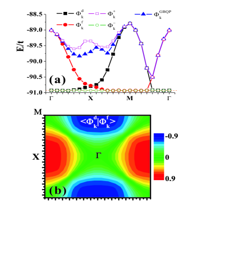
Figure 1: (a) Two-particle dispersions of different excited states for the $t-t^{\prime}-t^{\prime\prime}-J$ model doping two holes in $16\times 16$ lattice. The orange dashed line denotes the $d$-RVB state ($E_{dRVB}=-90.93t$). The symbols for momenta: $\Gamma\equiv(0.5,0.5)$, $X\equiv(5.5,0.5)$ and $M\equiv(5.5,5.5)$ in terms of $\pi/8$. (b) The momentum-space contour plot of the overlap between $|\Phi_{k}^{d}\rangle$ and $|\Phi_{k}^{f}\rangle$.

3 Results and discussion

Since the projections are included in Eqs.(14), the trial states $|\Phi_{\mathbf{k}}^{d}\rangle$ and $|\Phi_{\mathbf{k}}^{f}\rangle$ are no longer orthogonal. We need to diagonalize a $2\times 2$ Hamiltonian matrix in the subspace spanned by Eqs.(14). In principle, we can reconstruct two orthogonal states, $|\hat{\Phi}_{\mathbf{k}}^{d}\rangle$ and $|\hat{\Phi}_{\mathbf{k}}^{f}\rangle$, for each momentum by using Gram-Schmidt method. The Hamiltonian matrix in this subspace is given by

$$\hat{H}_{sub}=\left(\begin{array}[]{cc}H_{dd}&H_{df}\\ H_{fd}&H_{ff}\\ \end{array}\right),$$ (16)

where $H_{ij}\equiv\langle\hat{\Phi}_{\mathbf{k}}^{i}|\hat{H}|\hat{\Phi}_{\mathbf{k}}^{j}\rangle$ and $i,j=d$ or $f$. We further diagonalize $\hat{H}_{sub}$ to obtain the eigenstates $|\Phi_{\mathbf{k}}^{-}\rangle$ and $|\Phi_{\mathbf{k}}^{+}\rangle$ as a linear combination of $|\hat{\Phi}_{\mathbf{k}}^{d}\rangle$ and $|\hat{\Phi}_{\mathbf{k}}^{f}\rangle$. Without the projection, Eq.(13) provides a route to construct the BCS ground state and the two-particle excited state by using a linear combination of two orthonormal states $|\Psi_{\mathbf{k}}^{d}\rangle$ and $|\Psi_{\mathbf{k}}^{f}\rangle$. Therefore, we can expect the ground state $|\Phi_{\mathbf{k}}^{-}\rangle$ and the GQP excited state $|\Phi_{\mathbf{k}}^{+}\rangle$ should play the same role in the cases under the projection. A further question is whether the GBQP wave function $|\Phi_{\mathbf{k}}^{GBQP}\rangle$ mentioned above is appropriate to describe the two-particle excitation from the $d$-RVB state $|\Phi_{0}\rangle$. In Fig.1(a), we compare the dispersion of four different states discussed above with $|\Phi_{\mathbf{k}}^{GBQP}\rangle$. First, it is obvious that $|\Phi_{\mathbf{k}}^{-}\rangle$ exactly reproduces the optimized energy of the $d$-RVB state indicated by the orange dashed line. Based on this agreement, we are confident that $|\Phi_{\mathbf{k}}^{+}\rangle$ should properly represent the two-particle GQP excitation. Interestingly, except the deviation near the antinodal regions, the energy dispersion of $|\Phi_{\mathbf{k}}^{+}\rangle$ coincides with $|\Phi_{\mathbf{k}}^{GBQP}\rangle$ very well. We shall return to this deviation in the following. Here we see that $|\Phi_{\mathbf{k}}^{GBQP}\rangle$ has the lower energy than $|\Phi_{\mathbf{k}}^{+}\rangle$ around the regions with large $d$-wave pairing amplitude. Therefore, we may conclude that the GQP excitation seems reasonable to be constructed by applying BQP operators to the $d$-RVB wave function although $|\Phi_{\mathbf{k}}^{+}\rangle$ just represents the first two-particle GQP excited state.

Second, we notice that $|\Phi_{\mathbf{k}}^{d}\rangle$ ($|\Phi_{\mathbf{k}}^{f}\rangle$) shows dispersionless behavior inside (outside) the underlying Fermi surface. This results can be easily understood by transforming the representation (df) back to (c). In the original representation (c), they are given by

$$|\Phi_{\mathbf{k}}^{d}\rangle = \hat{P}_{N_{e}}\hat{P}_{G}c^{\dagger}_{\mathbf{k}\uparrow}c^{\dagger}_{-\mathbf{k}\downarrow}\prod_{\mathbf{q\neq k}}\left(u_{\mathbf{q}}+v_{\mathbf{q}}c^{\dagger}_{\mathbf{q}\uparrow}c^{\dagger}_{-\mathbf{q}\downarrow}\right)|0\rangle_{(c)},$$

$$|\Phi_{\mathbf{k}}^{f}\rangle = \hat{P}_{N_{e}}\hat{P}_{G}\prod_{\mathbf{q\neq k}}\left(u_{\mathbf{q}}+v_{\mathbf{q}}c^{\dagger}_{\mathbf{q}\uparrow}c^{\dagger}_{-\mathbf{q}\downarrow}\right)|0\rangle_{(c)}.$$ (17)

Apparently, there is an additional electron (hole) pair in $|\Phi_{\mathbf{k}}^{d}\rangle$ ($|\Phi_{\mathbf{k}}^{f}\rangle$) so that it only can show the dispersion outside (inside) the underlying Fermi surface in Fig.1(a). Next, we study the overlap between $|\Phi_{\mathbf{k}}^{d}\rangle$ and $|\Phi_{\mathbf{k}}^{f}\rangle$ shown in Fig.1(b). Note that without the projection, $|\Psi_{\mathbf{k}}^{d}\rangle$ and $|\Psi_{\mathbf{k}}^{f}\rangle$ are orthogonal for every momentum. Under the projection the overlap dramatically enhances near the antinodal regions. The shape of the overlap in the momentum space is very similar to the $d$-wave form factor, $\cos\mathbf{k_{x}}-\cos\mathbf{k_{y}}$, and the maxima about $0.82$ right at antinodes. It can be easily understood from Eq.(17) in the original representation (c). Since there is an extra Cooper pair $c^{\dagger}_{\mathbf{k}\uparrow}c^{\dagger}_{-\mathbf{k}\downarrow}$ in the overlap, we can expect that Gutzwiller’s projection would influence the Cooper pair following the $d$-wave symmetry in BCS wave functions. Thus, we can further comprehend the deviation for the excitation energy near the antinodal regions in Fig.1(a).

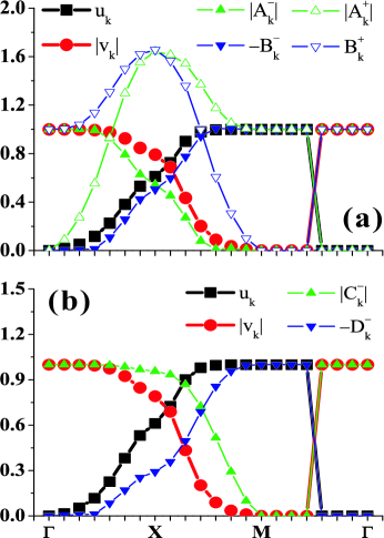
Figure 2: The coefficients (a) $A_{\mathbf{k}}^{\pm}$ and $B_{\mathbf{k}}^{\pm}$; (b) $C_{\mathbf{k}}^{\pm}$ and $D_{\mathbf{k}}^{\pm}$ along the high-symmetric momenta. Their definitions are explained in the text. The BCS coherence factors $u_{k}$ and $v_{k}$ obtained from the optimized parameters are shown for comparison.

Furthermore, it is important to examine the details of the eigenstates $|\Phi_{\mathbf{k}}^{\pm}\rangle$. We can write down $|\Phi_{\mathbf{k}}^{\pm}\rangle$ as a linear combination of the orthogonal states $|\hat{\Phi}_{\mathbf{k}}^{d/f}\rangle$:

$$|\Phi_{\mathbf{k}}^{\pm}\rangle=C_{\mathbf{k}}^{\pm}|\hat{\Phi}_{\mathbf{k}}^{d}\rangle+D_{\mathbf{k}}^{\pm}|\hat{\Phi}_{\mathbf{k}}^{f}\rangle,$$ (18)

where the coefficients $C_{\mathbf{k}}^{\pm}$ and $D_{\mathbf{k}}^{\pm}$ can be easily determined by diagonalizing Eq.(16). By using Gram-Schmidt method, the two orthogonal states $|\hat{\Phi}_{\mathbf{k}}^{d/f}\rangle$ can be written as

$$|\hat{\Phi}_{\mathbf{k}}^{d}\rangle = |\Phi_{\mathbf{k}}^{d}\rangle,$$

$$|\hat{\Phi}_{\mathbf{k}}^{f}\rangle = \frac{|\Phi_{\mathbf{k}}^{f}\rangle-\langle\Phi_{\mathbf{k}}^{d}|\Phi_{\mathbf{k}}^{f}\rangle|\Phi_{\mathbf{k}}^{d}\rangle}{\sqrt{1-|\langle\Phi_{\mathbf{k}}^{d}|\Phi_{\mathbf{k}}^{f}\rangle|^{2}}}.$$ (19)

Thus, the eigenstates $|\Phi_{\mathbf{k}}^{\pm}\rangle$ are expressed in terms of $|\Phi_{\mathbf{k}}^{d/f}\rangle$ as well,

$$|\Phi_{\mathbf{k}}^{\pm}\rangle=A_{\mathbf{k}}^{\pm}|\Phi_{\mathbf{k}}^{d}\rangle+B_{\mathbf{k}}^{\pm}|\Phi_{\mathbf{k}}^{f}\rangle.$$ (20)

Here the coefficients $A_{\mathbf{k}}^{\pm}$ and $B_{\mathbf{k}}^{\pm}$ are related to $C_{\mathbf{k}}^{\pm}$ and $D_{\mathbf{k}}^{\pm}$ according to Eq.(19). Note that the normalization condition guarantees $|C_{\mathbf{k}}^{\pm}|^{2}+|D_{\mathbf{k}}^{\pm}|^{2}=1$ but not necessary for $A_{\mathbf{k}}^{\pm}$ and $B_{\mathbf{k}}^{\pm}$.

In order to understand how Gutzwiller’s projection affects the coherence factors in Eq.(13), we plot the comparison between the BCS coherence factors and the coefficients $A_{\mathbf{k}}^{\pm}$ and $B_{\mathbf{k}}^{\pm}$ in Fig.2(a). We should notice that $u_{\mathbf{k}}$ and $v_{\mathbf{k}}$ are obtained from the optimized variational parameters. To avoid the confusion arising from the sign of $d$-wave symmetry, we show the absolute value of $v_{\mathbf{k}}$ and $A_{\mathbf{k}}^{\pm}$. Along the nodal direction, interestingly, the projection seems not to change the BCS coherence factors. This may imply the intimate relation between Gutzwiller’s projection and the $d$-wave gap function. However, since the coefficients $A_{\mathbf{k}}^{\pm}$ and $B_{\mathbf{k}}^{\pm}$ are not normalized, there is a large enhancement for the first GQP excited state and small suppression for the $d$-RVB ground state around the antinodal parts. In Fig.2(b), we clearly demonstrate the shape of the coefficients $C_{\mathbf{k}}^{\pm}$ and $D_{\mathbf{k}}^{\pm}$ looks similar to the BCS coherence factors in spite of the existence of Gutzwiller’s projection. The crossing curve of $C_{\mathbf{k}}^{\pm}$ and $D_{\mathbf{k}}^{\pm}$ bends more like a hole pocket at $(\pi,\pi)$, and however the BCS coherence factor displays a diamond-like underlying Fermi surface (not shown). Even so, it is reasonable to believe that the GQPs in the $d$-RVB wave function are still analogous to the BQP picture.

4 Conclusion

In conclusions, we have developed a method to examine the idea of BQPs in Gutzwiller-projected BCS wave functions. By calculating the two-particle excitation dispersion using VMC approach, the GQP excited states have been obtained. We have found the GBQP $|\Phi_{\mathbf{k}}^{GBQP}\rangle$ shows almost the same energy as the GQP $|\Phi_{\mathbf{k}}^{+}\rangle$ except that gives the lower energy around the antinodal regime. The reason is that there exists large overlap between $|\Phi_{\mathbf{k}}^{d}\rangle$ and $|\Phi_{\mathbf{k}}^{f}\rangle$ near the antinodes, suggesting the intimate connection between Gutzwiller’s projection and $d$-wave Cooper pairing. It also results in the deviation of the coefficients in $|\Phi_{\mathbf{k}}^{\pm}\rangle$ from the BCS coherence factors, which might be related to the nodal-antinodal dichotomy observed in cuprates by ARPES measurements. Therefore, the lower energy around the antinodal regions implies the GBQP excited wave functions are suitable to describe the low-lying excitations in strongly correlated superconductors.

5 Acknowledgments

The author thanks T.-K. Lee and Wei Ku for useful discussions. This work is supported by Brookhaven Science Associates, LLC under Contract No. DE-AC02-98CH10886 with the U.S. Department of Energy and the Postdoctoral Research Abroad Program sponsored by National Science Council in Taiwan with Grant No. NSC 101-2917-I-564-010.

References

- [1] I. M. Vishik et al., New J. Phys. 12, 105008 (2010).
- [2] P. A. Lee, N. Nagaosa, and X.-G. Wen, Rev. Mod. Phys. 78, 17 (2006).
- [3] P. Phillips, Rev. Mod. Phys. 82, 1719 (2010).
- [4] P. W. Anderson, Science 235, 1196 (1987).
- [5] J. K. Jain and P. W. Anderson, Proc. Nat. Acad. Sci. 106, 9131 (2009).
- [6] B. S. Shastry, Phys. Rev. B 81, 045121 (2010).
- [7] H. Matsui et al., Phys. Rev. Lett. 90, 217002 (2003).
- [8] Y. Ohta, T. Shimozato, R. Eder, and S. Maekawa, Phys. Rev. Lett. 73, 324 (1994).
- [9] S. Yunoki, E. Dagotto, and S. Sorella, Phys. Rev. Lett. 94, 037001 (2005).
- [10] S. Yunoki, Phys. Rev. B 72, 092505 (2005).
- [11] S. Yunoki, Phys. Rev. B 74, 180504 (2006).
- [12] C. P. Nave, D. A. Ivanov, and P. A. Lee, Phys. Rev. B 73, 104502 (2006).
- [13] K.-Y. Yang et al., Phys. Rev. B 73, 224513 (2006).
- [14] Chung-Pin Chou, T. K. Lee, and Chang-Ming Ho, Phys. Rev. B 74, 092503 (2006).
- [15] F. Tan and Q.-H. Wang, Phys. Rev. Lett. 100, 117004 (2008).
- [16] X. J. Zhou et al., Phys. Rev. Lett. 92, 187001 (2004).
- [17] J. Graf et al., Nature Physics 7, 805 (2011).
- [18] B. Edegger, V. N. Muthukumar and C. Gros, Adv. Phys. 56, 927 (2007).
- [19] M. Ogata and H. Fukuyama, Rep. Prog. Phys. 71, 036501 (2008).
- [20] C.-P. Chou, N. Fukushima, and T.-K. Lee, Phys. Rev. B 78, 134530 (2008).
- [21] H. Yokoyama and H. Shiba, J. Phys. Soc. Jpn. 57, 2482 (1988).
- [22] C.-P. Chou, F. Yang, and T.-K. Lee, Phys. Rev. B 85, 054510 (2012).
- [23] S. Sorella, Phys. Rev. B 64, 024512 (2001).