Curvaton mechanism after multi-field inflation

Abstract

The evolution of the curvature perturbation after multi-field inflation is studied in the light of the curvaton mechanism. Past numerical studies show that many-field inflation causes significant evolution of the curvature perturbation after inflation, which generates significant non-Gaussianity at the same time. We reveal the underlying mechanism of the evolution and show that the evolution is possible in a typical two-field inflation model.

I Introduction

The primordial curvature perturbation $\zeta(k)$ is strongly constrained by observation and provides a unique window on the very early universe Lyth-book . It is known to have the spectrum ${\cal P}_{\zeta}(k)\simeq(5\times 10^{-5})^{2}$ with spectral tilt $n-1\equiv d\ln{\cal P}_{\zeta}/d\ln k\simeq-0.04$, and in future one could detect the running $dn/d\ln k$ as well as non-Gaussianity signaled by the bispectrum and trispectrum.

The process of generating $\zeta$ begins presumably during inflation, when the vacuum fluctuations of one or more bosonic fields are converted to classical perturbations. Within this general framework, there exist many proposals Lyth-book .

One proposal is to use two or more inflaton fields, which drive inflation in the multi-field model. That paradigm has been widely investigated, but it has usually been supposed that $\zeta(x,t)$ evaluated at an epoch $t_{\mathrm{end}}$ just before (or sometimes just after) the end of inflation is to be identified with the observed quantities in the spectrum. For this reason, a great deal of effort has gone into the calculation of the spectrum, bispectrum and trispectrum of $\zeta$ at the end of inflation Multi1 ; Multi2 ; Multi3 ; Multi4 ; Multi5 ; Multi6 ; Multi-matsuda ; Multi-NG .

The evolution after many-field inflation has been studied numerically in Ref. CGJ using the statistical distribution of the parameters Easther:2005zr ; Battefeld:2008bu . Later in Ref. afterCGJ the evolution of the non-Gaussianity has been investigated. In these studies it has been found that there is a minimal number of the inflaton field $N_{f}\geq 10^{3}$, which is needed to realize the late-time creation and the domination of the curvature perturbation. Also, the number $N_{f}$ has been related to the creation of the non-Gaussianity. On the other hand, the calculation is not analytic and it is not clear if the evolution is possible in a two (or a few)-field model.

In this paper, we point out that the actual calculation of the curvature perturbation might well depend on the evolution after multi-field inflation, even if the number $N_{f}$ is not large. We show that the minimum number is $N_{f}=2$, simply because the mechanism requires isocurvature perturbation.

Just for simplicity, consider $N_{f}=2$ with the light scalar fields ($\phi,\sigma$) during inflation. The adiabatic and the entropy directions of multi-field inflation are defined using those fields. Basically, the “inflaton” (the adiabatic field) is not identical to $\phi$, even if $\sigma$ plays the role of the curvaton. The mixing is negligible when $\sigma$ is much lighter than $\phi$; that is the limit where the usual curvaton scenario applies.

Alternatively, it is possible to consider the opposite limit, where the fields have nearly equal mass. Can the curvaton mechanism work in that limit? A naive speculation is that the biased initial condition ($\sigma/\phi\ll 1$) might lead to the curvaton mechanism in that limit. Indeed the speculation is correct; however to reach the correct conclusion we need quantitative calculation of the curvaton mechanism in the equal-mass limit. The calculation details are shown in the Appendix. The usual curvaton mechanism is reviewed in Sec.II, and the non-linear formalism of the curvaton mechanism is reviewed in Sec.III. The basic idea of the equal-mass curvaton model is shown in Sec.IV for two-field inflation. Deviation from the equal-mass limit and the applications are discussed in Sec.V.

II Curvaton mechanism

In this section we review $\delta N$ formalism used to calculate $\zeta$. To define $\zeta$ one smooths the energy density $\rho$ on a super-horizon scale shorter than any scale of interest. Then it satisfies the local energy continuity equation,

$$\frac{\partial\rho(x,t)}{\partial t}=-\frac{3}{a(x,t)}\frac{\partial a(x,t)}{\partial t}\left(\rho(x,t)+p(x,t)\right),$$ (1)

where $t$ is time along a comoving thread of spacetime and $a$ is the local scale factor. Choosing the slicing of uniform $\rho$, the curvature perturbation is $\zeta\equiv\delta(\ln a)$ and

$$\frac{\partial\zeta(x,t)}{\partial t}=\delta\left(\frac{\dot{\rho}(t)}{\rho(t)+p(x,t)}\right).$$ (2)

If $p$ is a function purely of $\rho$, one will find $\dot{\zeta}=0$. That is the case of single field inflation when no other field perturbation is relevant. The inflaton field $\phi(x,t)$ determines the future evolution of both $\rho$ and $p$. Similarly, the component perturbations $\zeta_{i}$ are conserved if they scale like matter ($\rho_{m}\propto a^{-3}$) or radiation ($\rho_{r}\propto a^{-4}$).

During nearly exponential inflation, the vacuum fluctuation of each light scalar field $\phi_{i}$ is converted at horizon exit to a nearly Gaussian classical perturbation with spectrum $(H/2\pi)^{2}$, where $H\equiv\dot{a}(t)/a(t)$ in the unperturbed universe. Writing

$$\zeta=\delta[\ln(a(x,t)/a(t_{1})]\equiv\delta N,$$ (3)

and taking $t_{*}$ to be an epoch during inflation after relevant scales leave the horizon, we define $N(\phi_{1}(x,t_{*}),\phi_{2}(x,t_{*}),\cdots,t,t_{*})$ so that

$$\zeta(x,t)=N_{i}\delta\phi_{i}(x,t_{*})+\frac{1}{2}N_{ij}\delta\phi_{i}(x,t_{*})\delta\phi_{j}(x,t_{*})+\cdots,$$ (4)

where a subscript $i$ denotes $\partial/\partial\phi_{i}$ evaluated on the unperturbed trajectory. We find

$$n-1 = \frac{2\sum_{i}N_{i}N_{j}\eta_{ij}}{\sum_{m}N_{m}^{2}}-2\epsilon-\frac{2}{M_{p}^{2}\sum_{m}N_{m}^{2}}$$ (5)

$$\eta_{ij} \equiv M_{p}^{2}V_{ij}/V,\qquad\epsilon\equiv M_{p}^{2}\sum_{m}V_{m}^{2}/V^{2},$$ (6)

where $M_{p}$ is the reduced Planck mass.

The standard curvaton model lm ; curvaton-paper assumes that these expressions are dominated by the single ‘curvaton’ field $\sigma$, which starts to oscillate during radiation domination at a time when the component perturbation $\zeta_{\sigma}$ has negligible contribution to the curvature perturbation. Then the non-Gaussianity parameter is given by Lyth-gfc ; Lyth-general

$$f_{NL} \simeq \frac{5}{4r_{\sigma}}\left(1+\frac{g^{\prime\prime}g}{g^{2}}\right)-\frac{5}{3}-\frac{5}{6}r_{\sigma},$$ (7)

where $g(\sigma)$ is the initial amplitude of the oscillation as a function of the curvaton field at horizon exit Lyth-gfc . Here $r_{\sigma}$ is identical to $r_{1}$, which will be defined in this paper.

III Non-linear formalism and the evolution of the perturbation

In this paper we consider a clear separation of the adiabatic and the entropy perturbations in a two-field inflation model. The non-linear formalism for the component curvature perturbation is defined in Ref. Lyth-general ; Langlois:2008vk as

$$\zeta_{i} = \delta N+\int^{\rho}_{\bar{\rho}_{i}}H\frac{d\tilde{\rho}_{i}}{3(1+w_{i})\tilde{\rho}_{i}}$$ (8)

$$= \delta N+\frac{1}{3(1+w_{i})}\ln\left(\frac{\rho_{i}}{\bar{\rho}_{i}}\right)$$

$$\simeq \delta N+\frac{1}{3(1+w_{i})}\frac{\delta\rho_{i}^{\mathrm{iso}}}{\bar{\rho}_{i}},$$

where $w_{i}=1/3$ for the radiation fluid and $w_{i}=0$ for the matter fluid. Here a bar is for a homogeneous quantity, and the curvature perturbation of the total fluid should be discriminated from the component curvature perturbation $\zeta_{i}$. The quantity $\delta\rho_{i}^{\mathrm{iso}}=\rho_{i}-\bar{\rho}_{i}$ in Eq.(8) is the isocurvature perturbation (the fraction perturbation that satisfies $\sum\delta\rho_{i}^{\mathrm{iso}}\equiv 0$), which is defined on the uniform density hypersurfaces.

In order to formulate the evolution of the curvature perturbation, which is caused by the adiabatic-isocurvature mixings, we need to define first the “starting point” perturbations at an epoch.

III.1 The primordial perturbations

For the first step, we define the primordial quantities. In this paper the quantities at the end of inflation are denoted by the subscript “end”, while the corresponding scale exited horizon at $t_{*}$. The subscript “$*$” is used for the quantities at the horizon exit. For our purpose, we define the primordial curvature and isocurvature perturbations at the end of the primordial inflation.

We find from Eq.(8);

$$\rho_{i} = \bar{\rho}_{i}e^{3(1+w_{i})(\zeta_{i}-\delta N)}$$ (9)

$$\simeq \bar{\rho}_{i}+3(1+w_{i})\zeta_{i}^{\mathrm{iso}}\bar{\rho}_{i}$$

$$\equiv \bar{\rho}_{i}+\delta\rho_{i}^{\mathrm{iso}}.$$

Then we find from $\rho^{\mathrm{tot}}\equiv\rho_{1}+\rho_{2}=\bar{\rho}_{1}+\bar{\rho}_{2}$:

$$f_{1}e^{3(1+w_{1})(\zeta_{1}-\delta N)}+\left(1-f_{1}\right)e^{3(1+w_{2})(\zeta_{2}-\delta N)}=1,$$ (10)

where the fraction of the energy density is defined by

$$f_{1}\equiv\frac{\bar{\rho}_{1}}{\bar{\rho}_{1}+\bar{\rho}_{2}}.$$ (11)

Expanding Eq.(10) and solving the equation for $\delta N$, we find at first order Lyth-general

$$\delta N = r_{1}\zeta_{1}+(1-r_{1})\zeta_{2}$$ (12)

$$\equiv \left[r_{1}\zeta_{1}^{\mathrm{iso}}+(1-r_{1})\zeta_{2}^{\mathrm{iso}}\right]+\zeta^{\mathrm{adi}},$$

where $\zeta^{\mathrm{iso}}_{i}$ denotes the second component in Eq.(8). $r_{1}$ is defined by

$$r_{1}\equiv\frac{3(1+w_{1})\bar{\rho}_{1}}{3(1+w_{1})\bar{\rho}_{1}+3(1+w_{2})\bar{\rho}_{2}}.$$ (13)

Defining the primordial adiabatic curvature perturbation ($\zeta^{\mathrm{inf}}$) just at the end of inflation, the component curvature perturbation ($\zeta_{i}$) can be split into $\zeta^{\mathrm{inf}}$ and $\zeta_{i}^{\mathrm{iso}}$.

The obvious identity is

$$r_{1,\mathrm{end}}\zeta_{1,\mathrm{end}}^{\mathrm{iso}}+(1-r_{1,\mathrm{end}})\zeta_{2,\mathrm{end}}^{\mathrm{iso}}\equiv 0,$$ (14)

which is valid at the end of inflation. Apart from that point the deviation due to the evolution of $r_{1}$ becomes significant.

The parameter of the fluid ($w_{i}$) is constant when $\rho_{i}$ behaves like matter ($w_{i}=0$) or radiation ($w_{i}=1/3$), and a jump (e.g, $w_{i}=0\rightarrow w_{i}=1/3$) is possible when instant transition is assumed. In this paper we are using the sudden-decay approximation for the curvaton mechanism.  We also assume that the inflatons start sinusoidal oscillations just at the end of slow-roll.

The curvature perturbation in the standard curvaton scenario is usually expressed as

$$\delta N=r_{1}\zeta_{1}+(1-r_{1})\zeta^{\mathrm{inf}}.$$ (15)

Assuming that $\zeta_{1}^{\mathrm{iso}}\gg\zeta^{\mathrm{inf}}\gg\zeta_{2}^{\mathrm{iso}}$, one will find $\zeta_{1}\simeq\zeta_{1}^{\mathrm{iso}}$ and $\zeta_{2}\simeq\zeta^{\mathrm{inf}}$, which gives Eq.(15) from Eq.(12). Usually the above approximation is justified when $m_{1}\ll m_{2}$ and the curvaton is negligible during inflation.

In this paper we are considering the equal-mass limit ($m_{1}\simeq m_{2}$), which is in the opposite limit of the conventional curvaton. In Appendix we show the validity of the above approximations and derive the quantitative bound on the ratio $\phi_{1}/\phi_{2}$.

IV A basic model

In this section we show why the curvaton mechanism can create the dominant part of the curvature perturbation after conventional chaotic multi-field inflation, neither by adding extra light field (curvaton) nor by introducing many inflatons. The calculation clearly explains why and how the curvaton mechanism works in the equal-mass limit ($m_{1}\simeq m_{2}$).

We assume (for simplicity) that after inflation the field $\phi_{2}$ decays immediately into radiation and $\phi_{1}$ starts sinusoidal oscillation at the same time. Then $\phi_{1}$ decays late at $H_{d1}\ll H_{I}$. There is no mixing between these components. Here $H_{I}$ denotes the Hubble parameter during primordial inflation.

In this scenario, we consider two phases $(A,B)$ characterized by $w_{1A}=0$ and $w_{1B}=1/3$. Here the subscripts $A$ and $B$ denotes the quantities in the phase A and B. They are separated by the uniform density hypersurface $H_{d1}\simeq\Gamma_{1}$:

1. $\rho_{1}$; oscillation, $\rho_{2}$; radiation
   ($w_{1}=0$, $w_{2}=1/3$)

2. Radiation
   ($w_{1}=w_{2}=1/3$).

The important assumption of the model is that the transition occurs on the uniform density hypersurfaces so that we can neglect additional creation of $\delta N$ (modulation) at the transition.

We find in phase (A);

$$\delta N \equiv r_{1A}\zeta_{1A}+(1-r_{1A})\zeta_{2},$$ (16)

where the subscript “$A$” (or “$B$”) is omitted for $\zeta_{2}$, since $\zeta_{2}$ is constant during the evolution. Here we used the definition

$$r_{1A}=\frac{3\bar{\rho}_{1}}{3\bar{\rho}_{1}+4\bar{\rho}_{2}}.$$ (17)

Consider a simple double-quadratic chaotic inflation model in the equal-mass limit. The potential is given by

$$V(\phi_{1},\phi_{2})=\frac{1}{2}m^{2}\left(\phi_{1}^{2}+\phi_{2}^{2}\right)\equiv\frac{1}{2}m^{2}\phi_{r}^{2},$$ (18)

where $\phi_{1,2}$ are real scalar fields. Besides the potential, we need the interaction that causes difference in the decay rates. Fig.1 shows the evolution of the densities after inflation.

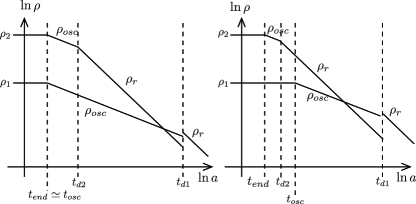
Figure 1: $t_{\mathrm{end}}$, $t_{d2}$, $t_{\mathrm{osc}}$ and $t_{d1}$ denote the time at the end of inflation, $\phi_{2}$ decay, the beginning of $\phi_{1}$ oscillation and $\phi_{1}$ decay, respectively. Our scenario is shown in the left-hand side, which gives the time-ordering $t_{end}\simeq t_{osc}<t_{d2}<t_{d1}$. The usual curvaton scenario is shown in the right-hand side, which gives $t_{end}<t_{d2}<t_{osc}<t_{d1}$.

The end of chaotic inflation is given by

$$\phi_{1,\mathrm{end}}^{2}+\phi_{2,\mathrm{end}}^{2}\equiv\phi_{r,\mathrm{end}}^{2}\simeq M_{p}^{2}.$$ (19)

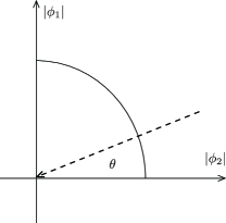
Figure 2: The straight dotted line with an arrow is the inflaton trajectory, and the circle gives the uniform-density surface along which the entropy perturbation $\delta s$ appears.

Since the potential is quadratic during inflation, we find

$$\zeta^{\mathrm{inf}}=\frac{1}{\eta}\frac{\delta\phi_{r*}}{\phi_{r*}}.$$ (20)

In this section we consider $\theta\ll 1$, which leads to the simplifications $\sin\theta\sim\theta$ and $\cos\theta\sim 1$. Our approximations are based on the exact calculation in Appendix A.

From Eq.(81), we find the component perturbation of the late-decaying component ($\phi_{1}$) at the end of inflation:

$$\zeta_{1A}\simeq\frac{1}{3}\frac{\delta\rho_{1,\mathrm{end}}^{\mathrm{iso}}}{\bar{\rho}_{1,\mathrm{end}}}\simeq\frac{2}{3}\frac{\delta\theta}{\bar{\theta}}+\frac{1}{3}\left(\frac{\delta\theta}{\bar{\theta}}\right)^{2}.$$ (21)

The usual approximation of the curvaton mechanism is $\zeta_{1A}^{\mathrm{iso}}\gg\zeta^{\mathrm{inf}}$. The validity of this approximation is examined in the Appendix.

From Eq.(83), the final curvature perturbation is

$$\zeta^{\mathrm{fin}}\simeq\frac{2r_{1-}}{3}\left[\frac{\delta\theta}{\bar{\theta}}+\frac{1}{2}\left(\frac{\delta\theta}{\bar{\theta}}\right)^{2}\right].$$ (22)

Defining the ratio $y\equiv\sqrt{\Gamma_{1}/\Gamma_{2}}$, $r_{1-}$ ($r_{1}$ evaluated in the phase (A) just before the decay) is given by

$$r_{1-}\simeq\frac{3\bar{\theta}^{2}}{3\bar{\theta}^{2}+4y}.$$ (23)

The non-Gaussianity parameter has been calculated in Ref. Lyth-general . We find for $\theta\ll 1$:

$$f_{NL} \simeq \frac{5}{4r_{1}}\left(1+\frac{g^{\prime\prime}g}{g^{2}}\right)-\frac{5}{3}-\frac{5}{6}r_{1}$$ (24)

$$\sim \frac{5}{4r_{1-}}.$$

Further simplification is possible when $\delta\theta=\delta s_{*}/\phi_{r*}$ and ${\cal P}_{\delta s_{*}}={\cal P}_{\delta\phi_{r*}}$. For the quadratic potential we have $\phi_{r*}=2\sqrt{N_{e}}M_{p}\gg\phi_{e,\mathrm{end}}$, where $N_{e}$ is the number of e-foldings during the primordial inflation spent after the corresponding scale exits horizon. The condition of the curvaton mechanism $\zeta^{\mathrm{fin}}>\zeta^{\mathrm{inf}}$ gives

$$\bar{\theta}<\frac{2}{3}r_{1-}\eta\simeq\frac{5}{6}\frac{\eta}{f_{NL}}.$$ (25)

Here $\bar{\theta}$ should be less than 1 but does not require many orders of magnitude. From the CMB spectrum we find the normalization given by

$${\cal P}^{1/2}_{\zeta^{\mathrm{fin}}}\simeq\frac{r_{1-}}{6\pi\sqrt{N_{e}}\bar{\theta}}\frac{H_{I}}{M_{p}}\simeq 5\times 10^{-5}.$$ (26)

Using Eq.(25), we find

$$\frac{H_{I}}{M_{p}}<5\eta\times 10^{-3},$$ (27)

which does not always require significant suppression. The ratio $y\equiv\sqrt{\Gamma_{1}/\Gamma_{2}}$ is calculated in Eq.(86) and is given by

$$y\simeq\frac{3}{5}f_{NL}\theta^{2}.$$ (28)

We thus find that the difference between $\phi_{1}$ and $\phi_{2}$ decay rates is in the conceivable range.

The above conditions tell us how small $\theta$ and $y$ have to be to get a given CMB spectrum and $f_{NL}$. They have to be some orders of magnitude below 1 but not very many.

If the potential during inflation is both symmetric and quadratic, we find $\eta\equiv\eta_{1}=\eta_{2}$. We thus find the spectral index

$$n-1=-2\epsilon+\eta=0,$$ (29)

which shows that the above model requires deviation from the symmetric potential.

Looking back into the many-field inflation, the model in Ref. CGJ assumed that the inflaton masses are not exactly the same but may have statistical distribution around the mean value. In that case, the cancellation in the spectral index is not realistic. Since the deviation from the symmetric potential is expected, we need to examine what deviation is needed for the model. Then we can understand why and how the curvaton mechanism works in the many-field inflation model.

V Deviation from the symmetric potential

The deviation from the symmetric quadratic potential can be classified as follows;

1. A small mass difference ($1\lesssim m_{2}/m_{1}\lesssim 10$)

   The spectral index does not vanish when the double quadratic potential has different (but not so much different as the usual curvaton) mass. The slow-roll parameters are

   $$\epsilon_{H} \equiv \frac{\dot{H}}{H^{2}}=\sum\epsilon_{i}=\sum\eta_{i}f_{i}$$

   $$\eta_{i} \equiv \frac{m_{i}^{2}}{3H_{I}^{2}},$$ (30)

   where the fraction of the density is given by $f_{i}\equiv\frac{\rho_{i*}}{\rho_{\mathrm{tot*}}}$. The spectral index is shifted from $n_{s}-1=0$ and is given by

   $$n_{s}-1 = -2\epsilon_{H}+2\eta_{1}$$ (31)

   $$\simeq -2[\eta_{1}f_{1}+\eta_{2}(1-f_{1})]+2\eta_{1}$$

   $$\simeq -2(\eta_{2}-\eta_{1})$$

   $$\equiv -2P\eta_{2}$$

   $$= -\frac{P}{N_{e}},$$

   where $P\equiv\frac{m_{2}^{2}-m_{1}^{2}}{m_{2}^{2}}<1$. The observation WMAP7 shows $n_{s}-1=0.037\pm 0.014$, which suggests $N_{e}\lesssim 40$ and requires secondary inflation thermal-Inf .

   Besides the spectral index, $m_{1}<m_{2}$ suggests that the oscillation of the field $\phi_{1}$ is slightly delayed compared to $\phi_{2}$. The delay may enhance the density of $\phi_{1}$ at the beginning of the oscillation, while the initial $\rho_{1}$ density may be reduced since $m_{1}$ is smaller. Defining $y_{\mathrm{eff}}\equiv\sqrt{\Gamma_{1}/m_{1}}$ and $\theta_{\mathrm{eff}}\equiv\phi_{1}/\phi_{2}$ at the end of inflation, we find

   $$r_{1A-} \simeq \frac{3m_{1}^{2}\bar{\phi}_{1}^{2}}{3m_{1}^{2}\bar{\phi}_{1}^{2}+4m_{2}^{2}\bar{\phi}_{2}^{2}\left(\frac{m_{1}^{2}}{m_{2}^{2}}\right)y_{\mathrm{eff}}}$$ (32)

   $$\simeq \frac{3\bar{\theta}_{\mathrm{eff}}^{2}}{3\bar{\theta}_{\mathrm{eff}}^{2}+4y_{\mathrm{eff}}},$$

   which gives a similar bound for $\theta_{\mathrm{eff}}$ ($y_{\mathrm{eff}}$).

2. Heavy curvaton ($m_{1}\gtrsim m_{2}$)

   Usually the curvaton is assumed to be much lighter than the inflaton; however this assumption could be avoided. We consider the curvaton mechanism when the curvaton is slightly heavier than the inflaton.

   We assume $\rho_{2}>\rho_{1}$. Once it is assumed at the beginning of inflation, it remains true during inflation. Then $\phi_{1}$-oscillation starts during inflation. It begins when

   $$m_{1}^{2}=H^{2}_{\mathrm{osc}}\simeq\frac{m_{2}^{2}\phi_{2}^{2}|_{\mathrm{osc}}}{6M_{p}^{2}},$$ (33)

   where the subscript “osc” denotes the beginning of $\phi_{1}$-oscillation. From the above equation and $\phi_{2}|_{\mathrm{osc}}\simeq 2\sqrt{N_{2}}M_{p}$, where $N_{2}$ is the remaining number of e-foldings after the beginning of $\phi_{1}$-oscillation, we find

   $$N_{2}=\frac{3m_{1}^{2}}{2m_{2}^{2}}.$$ (34)

   Defining $y_{\mathrm{eff}}\equiv e^{3N_{2}}\sqrt{\Gamma_{1}/\Gamma_{2}}$ and $\theta_{\mathrm{osc}}\equiv[\phi_{1}/\phi_{2}]_{\mathrm{osc}}$, we can estimate

   $$r_{1A-} \sim \frac{3\bar{\theta}_{\mathrm{osc}}^{2}}{3\bar{\theta}_{\mathrm{osc}}^{2}+4y_{\mathrm{eff}}}.$$ (35)

   Unfortunately, the spectral index is

   $$n_{s}-1 \simeq -2\epsilon_{H}+2\eta_{1}$$ (36)

   $$\simeq -2\eta_{2}+2\eta_{1}$$

   $$\simeq 2\eta_{1}>0.$$

3. Symmetric but Non-quadratic

   The potential could be dominated by a polynomial $V(\phi_{r})\propto\phi_{r}^{p}$ at the moment when the perturbation exits horizon, while it can be approximated by the quadratic potential during the oscillation. For the polynomial we find $\phi_{r*}\simeq\sqrt{2pN_{e}}M_{p}$ and the slow-roll parameters

   $$\epsilon_{H} \simeq \frac{1}{2}M_{p}^{2}\frac{p^{2}}{\phi_{r}^{2}}$$ (37)

   $$\eta_{1} \simeq M_{p}^{2}\frac{p(p-1)}{\phi_{r}^{2}}.$$ (38)

   The spectral index is shifted and is given by

   $$n_{s}-1 \simeq -\frac{M_{p}^{2}}{\phi_{r}^{2}}\left[p^{2}-2p(p-1)\right]$$ (39)

   $$\simeq \frac{p-2}{2N_{e}}.$$

   The result suggests that $p<2$ is needed for the scenario. In that case the mass and the coefficient of the polynomial must run in the trans-Planckian run-inf . $p=1$ would correspond to monodromy in the string theory and it requires $N_{e}\lesssim 20$. $p<1$ is an interesting possibility if the effective action allows fractional power.

V.1 A model with a complex scalar

An inderesting application of the idea is that a conventional 2-field multiplet contains both inflation and the curvaton at the same time. Consider a complex scalar field $\Phi\equiv\phi_{2}+i\phi_{1}$, which gives the symmetric potential

$$V(\Phi)=\frac{1}{2}m^{2}|\Phi^{2}|^{2}=\frac{1}{2}m^{2}(\phi_{1}^{2}+\phi_{2}^{2}).$$ (40)

First, consider a small symmetry breaking caused by

$$\Delta V\sim\frac{\Lambda^{4}}{M^{2}}\left(\frac{\Phi+\Phi^{*}}{2}\right)^{2},$$ (41)

where $\Lambda\ll M$ is assumed. $\phi_{2}$-oscillation may cause significant particle production when there is the interaction given by

$${\cal L}_{\mathrm{int}}=g(\Phi+\Phi^{*})\bar{\psi}\psi,$$ (42)

which can lead to significant $\psi$-production at the enhanced symmetric point ($\phi_{2}\sim 0$) PR . The coefficient of the interaction could be small ($g\sim\Lambda/M\ll 1$) when it is suppressed by a cut-off scale. $\psi$ may decay quickly into radiation since the amplitude of the oscillation after chaotic inflation is very large PR .

Define $\delta m^{2}\equiv\frac{2\Lambda^{4}}{M^{2}}$. If $\delta m^{2}$ is much smaller than $m^{2}$, the cancellation in Eq.(31) is still significant. On the other hand, it is possible to assume $\delta m^{2}/m^{2}\sim O(1)$ (which is still within the conventional set-up of multi-field inflation) one obtains $P\sim 1$ and $n_{s}-1\sim-\frac{1}{N_{e}}$. Again, the scenario requires additional inflation stage thermal-Inf .

Second, consider the case in which the potential during inflation is dominated by a polynomial $V(\Phi)\propto\Phi^{p}$. The curvaton can dominate the spectrum, however the spectral index becomes

$$n_{s}-1 \simeq -\frac{M_{p}^{2}}{\phi_{r}^{2}}\left[p^{2}-2p(p-1)\right]$$ (43)

$$\simeq \frac{p-2}{2N_{e}}.$$

The scenario requires $p<2$.

V.2 Sneutrino inflation

It is possible to assume small inflation “before” the multi-field inflation. The observed spectrum of the curvaton perturbation exits horizon during the first inflation. In that case $\epsilon_{H}$ is determined by the first inflation and the cancellation in the spectral index is avoided. This scenario uses multi-field inflation for the curvaton inflation Infcurv .

The usual sneutrino inflation Ellis:2003sq uses $m\sim 10^{13}$ GeV to satisfy the CMB normalization. When the condition is combined with the gravitino problem, Yukawa coupling of the first generation sneutrino (single-field inflaton) must satisfy $(Y_{\nu}Y_{\nu})^{\dagger}_{11}<10^{-12}$, whilst other Yukawa couplings will not be so small. Here $Y_{\nu}$ is the neutrino Yukawa matrix.

In this section we consider multi-stage inflation, in which three sneutrinos play crucial role. We assume that the first single-field inflation is caused by the third generation sneutrino, and the secondary two-field inflation is caused by the first and the second generation sneutrinos with the mass $M_{1}=M_{2}\equiv\hat{M}$. We assume $M_{3}>\hat{M}$ for the third generation.

The reheating after two-field inflation is due to the decay of the second generation sneutrino, which gives the reheating temperature

$$T_{R}=\left(\frac{90}{\pi^{2}g_{*}}\right)^{1/4}\sqrt{\Gamma_{2}M_{p}},$$ (44)

where the decay rate is

$$\Gamma_{i}\simeq\frac{1}{4\pi}\left(Y_{\nu}Y_{\nu}^{\dagger}\right)_{ii}\hat{M}.$$ (45)

From Eq.(71), the curvaton mechanism is significant when $\Gamma_{2}\gg\Gamma_{1}$. For the two-field sneutrino inflation, which is the secondary inflation of the above scenario, we find

$${\cal P}_{\zeta_{1}}^{1/2}<\frac{1}{3\pi}\left(\frac{(Y_{\nu}Y_{\nu}^{\dagger})_{22}}{(Y_{\nu}Y_{\nu}^{\dagger})_{11}}\right)^{1/4}\frac{\hat{M}}{M_{p}}.$$ (46)

Here the mass of the first (second) neutrino is

$$(m_{\nu})_{ii}\simeq(Y_{\nu}Y_{\nu}^{\dagger})_{ii}\frac{<H_{u}>^{2}}{\hat{M}}.$$ (47)

We thus find for the given neutrino mass $(m_{\nu})_{11}$ and $(m_{\nu})_{22}$;

$${\cal P}_{\zeta_{1}}^{1/2}<\frac{1}{3\pi}\left(\frac{(m_{\nu})_{22}}{(m_{\nu})_{11}}\right)^{1/4}\frac{\hat{M}}{M_{p}}.$$ (48)

The reheating temperature after inflation is given by

$$T_{R}=\left(\frac{45}{8\pi^{4}g_{*}}\right)^{1/4}\frac{\hat{M}}{<H_{u}>}\sqrt{(m_{\nu})_{22}M_{p}},$$ (49)

while the temperature just after the curvaton decay is

$$T_{R}^{\prime}=\left(\frac{45}{8\pi^{4}g_{*}}\right)^{1/4}\frac{\hat{M}}{<H_{u}>}\sqrt{(m_{\nu})_{11}M_{p}}.$$ (50)

We may write the spectrum ${\cal P}_{\zeta_{1}}$ using $T_{R}$ and $T_{R}^{\prime}$;

$${\cal P}_{\zeta_{1}}^{1/2}<\frac{1}{3\pi}\left(\frac{T_{R}}{T_{R}^{\prime}}\right)^{1/2}\frac{\hat{M}}{M_{p}}.$$ (51)

When the primary inflation gives the number of e-foldings $N_{1}$, the spectral index is

$$n_{s}-1\simeq-2\epsilon_{H}\simeq-\frac{1}{N_{1}}.$$ (52)

The observation gives $n_{s}-1=0.037\pm 0.014$, which suggests $20\lesssim N_{1}\lesssim 40$ for the first inflation.

V.3 N-flation

The two-field inflation model considered in this paper is a simplification of the N-flation model N-flation . The N-flation has been studied using statistical argument CGJ , which helps us understand the results obtained above for the two-field model.

Assuming (for simplicity) the same potential for all $N_{f}$ fields, we find

$$V(\phi_{n})=\sum^{N_{f}}_{n=1}\frac{1}{2}m^{2}\phi_{n}^{2}.$$ (53)

Using the adiabatic field defined by

$$\phi_{r}^{2}\equiv\sum^{N_{f}}_{n=1}\phi_{n}^{2},$$ (54)

we find the potential

$$V(\phi_{r})=\frac{1}{2}m^{2}\phi_{r}^{2}.$$ (55)

If we assume uniform initial condition $\phi_{n}\simeq\phi_{0}$, the model is identical to the two-field model with $\theta\sim 1/\sqrt{N_{f}}\ll 1$.

For the number of e-foldings $N_{e}\sim 60$, the usual curvature perturbation created at the horizon exit is given by

$$\zeta^{\mathrm{inf}}=-H_{I}\left.\frac{\delta\phi_{r}}{\dot{\phi}_{r}}\right|_{*}=2N_{e}\left.\frac{\delta\phi_{r}}{\phi_{r}}\right|_{*}.$$ (56)

where $H_{I}^{2}\equiv\frac{N_{f}m^{2}\phi_{0}^{2}}{6M_{p}^{2}}$ is the Hubble parameter during the primordial N-flation.

Suppose that the decay rate $\Gamma_{n}$ is uniform except for a field $\phi_{1}$, which has $\Gamma_{1}\ll\Gamma_{n}$. Here the density ratio becomes $r_{1}^{*}\simeq\frac{1}{N_{f}}$. Repeating the same calculation, we find

$$\zeta_{1}\equiv\frac{\delta\rho_{1}}{3\rho_{1}}=\frac{2}{3}\frac{\delta\phi_{1}}{\phi_{0}}\simeq\frac{2}{3}\sqrt{N_{f}}\frac{\delta s}{\phi_{r}}.$$ (57)

${\cal P}_{\zeta^{\mathrm{inf}}}^{1/2}\ll{\cal P}_{\zeta_{1}}^{1/2}$ is possible when $N_{f}\gg N_{e}^{2}$. This gives the minimum number of the fields that is needed for the curvaton mechanism and it explains the numerical calculation in Ref. CGJ .

In the above scenario, the curvaton is one of the inflaton fields that are equally participating $1/N_{f}$ of the inflaton dynamics.

At the end of inflation, the fraction of $\rho_{1}$ is

$$r_{1}(t_{end})=\frac{1}{N_{f}}\ll 1,$$ (58)

while at the decay of $\phi_{1}$ it can grow;

$$r_{1}(t_{decay})=r_{1}(t_{end})\times\left(\frac{\Gamma_{n}}{\Gamma_{1}}\right)^{1/2}.$$ (59)

We need for the curvaton mechanism (i.e, $\zeta_{1}$-domination)

$$\frac{2}{3}\sqrt{N_{f}}\frac{{\cal P}_{\delta\phi_{1}}}{\phi_{r}}\times\frac{1}{N_{f}}\left(\frac{\Gamma_{n}}{\Gamma_{1}}\right)^{1/2}>2N_{e}\frac{{\cal P}_{\delta\phi_{r}}}{\phi_{r}},$$ (60)

which leads to

$$\left(\frac{\Gamma_{1}}{\Gamma_{n}}\right)^{1/2}<\frac{1}{3N_{e}\sqrt{N_{f}}}.$$ (61)

Significant non-Gaussianity ($f_{NL}$) requires $r(t_{decay})\sim 0.1$, which gives

$$\left(\frac{\Gamma_{1}}{\Gamma_{n}}\right)^{1/2}\sim\frac{10}{N_{f}}.$$ (62)

If the distribution is statistical for the decay rate, we need $N_{f}\gg 1$ for the strong suppression ($\Gamma_{1}/\Gamma_{n}\ll 1$).

In this section we found that the evolution after inflation may dominate the curvature perturbation when $N_{f}$ is large. Our result explains the numerical calculation in Ref. CGJ .

VI Conclusions

The evolution after multi-field inflation can change the curvature perturbation. In this paper we considered a conventional two-field inflation model and showed that the curvaton mechanism after multi-field inflation could be significant when the decay rates are not identical . Interestingly, the mechanism works for a complex scalar field $\Phi\equiv\phi_{2}+i\phi_{1}$.

The previous numerical study CGJ showed that $N_{f}\gg 1$ causes significant evolution of the curvature perturbation after inflation as well as the creation of significant non-Gaussianity. We showed that the same is true for two-field inflation, in which $\theta\ll 1$ is required instead of $N_{f}\gg 1$.

The source of the curvaton mechanism is the entropy perturbation generated during multi-field inflation. Since the uniform density surface of the multi-field potential is flat by definition, the perturbation on that surface is inevitable.

Our results suggest that many-field inflation must be considered with care. A large number ($N_{f}\geq 10^{3}$) can easily explain the required condition for the curvaton domination.

VII Acknowledgment

We thank D. H. Lyth for collaboration in the early stage of the paper. T.M thanks J. McDonald for many valuable discussions. S.E. is supported by the Grant-in-Aid for Nagoya University Global COE Program, ”Quest for Fundamental Principles in the Universe: from Particles to the Solar System and the Cosmos”.

Appendix A Calculation details

A.1 Evolution of the curvature perturbation

In this Appendix we show the calculation details of the evolution after inflation.

We first assume that the potential is quadratic and symmetric during chaotic inflation. In our formalism $\zeta^{\mathrm{inf}}$ is defined at the end of inflation. The entropy perturbation is realized by $\delta\theta$, which is the perturbation of the angle $\theta$ in Fig.2.

The spectrum of the entropy perturbation during inflation is ${\cal P}_{\delta s_{*}}\simeq(H_{*}/2\pi)^{2}$. The entropy perturbation causes the fraction perturbation between densities. Using $\delta\theta$, the densities of the components and the isocurvature perturbations at the end of inflation are given by

$$\bar{\rho}_{1,\mathrm{end}} = \frac{1}{2}m^{2}|\phi_{r}^{\mathrm{end}}|^{2}\sin^{2}\bar{\theta}\simeq\frac{m^{2}M_{p}^{2}}{2}\sin^{2}\bar{\theta}$$ (64)

$$\delta\rho_{1,\mathrm{end}}^{\mathrm{iso}}\simeq m^{2}M_{p}^{2}(\sin\bar{\theta}\cos\bar{\theta})\delta\theta,$$

$$\bar{\rho}_{2,\mathrm{end}} = \frac{1}{2}m^{2}|\phi_{r}^{\mathrm{end}}|^{2}\cos^{2}\bar{\theta}\simeq\frac{m^{2}M_{p}^{2}}{2}\cos^{2}\bar{\theta}$$ (66)

$$\delta\rho_{1,\mathrm{end}}^{\mathrm{iso}}+\delta\rho_{2,\mathrm{end}}^{\mathrm{iso}}=0.$$

We find at the end of inflation:

$$f_{1} \equiv \frac{\bar{\rho}_{1}}{\bar{\rho}_{1}+\bar{\rho}_{2}}=\sin^{2}\bar{\theta},$$ (67)

$$\delta f_{1} \simeq \frac{\partial f_{1}}{\partial\theta}\delta\theta=2[\sin\bar{\theta}\cos\bar{\theta}]\delta\theta$$ (68)

$$= [\sin 2\bar{\theta}]\delta\theta.$$

The expansion with respect to $\delta\theta$ makes no sense when $\delta\theta/\sin\theta\geq 1$ or $\delta\theta/\cos\theta\geq 1$ Lyth-ngaus . We are excluding those regions.

Creation of the curvature perturbation after inflation requires the decay rate $\Gamma_{1}\ll\Gamma_{2}$. In the phase (A) we find

$$\zeta^{\mathrm{iso}}_{1A} \simeq \frac{2}{3}\frac{\cos\bar{\theta}}{\sin\bar{\theta}}\delta\theta$$ (69)

$$\zeta^{\mathrm{iso}}_{2A} \simeq -\frac{1}{2}\frac{\sin\bar{\theta}}{\cos\bar{\theta}}\delta\theta.$$ (70)

Using Eq.(12), we find

$$\zeta^{\mathrm{fin}} = \left[\frac{2}{3}r_{1-}\frac{\cos\bar{\theta}}{\sin\bar{\theta}}-\frac{1}{2}(1-r_{1-})\frac{\sin\bar{\theta}}{\cos\bar{\theta}}\right]\delta\theta+\zeta^{\mathrm{inf}}$$ (71)

$$= \left[\frac{4r_{1-}\cos^{2}\bar{\theta}-3(1-r_{1-})\sin^{2}\bar{\theta}}{6\sin\bar{\theta}\cos\bar{\theta}}\right]\delta\theta$$

$$+\zeta^{\mathrm{inf}},$$

where $r_{1-}$ denotes the value of $r_{1A}$ evaluated just before the end of the phase (A).

The evolution is

$$\bar{\rho}_{1-} = \left[\frac{m^{2}M_{p}^{2}}{2}\sin^{2}\bar{\theta}\right]\times\left(\frac{a_{\mathrm{d1}}}{a_{\mathrm{end}}}\right)^{-3}$$

$$\bar{\rho}_{2-} = \left[\frac{m^{2}M_{p}^{2}}{2}\cos^{2}\bar{\theta}\right]\times\left(\frac{a_{\mathrm{d2}}}{a_{\mathrm{end}}}\right)^{-3}\left(\frac{a_{\mathrm{d1}}}{a_{\mathrm{d2}}}\right)^{-4},$$ (72)

which leads to the ratio

$$\frac{\bar{\rho}_{2-}}{\bar{\rho}_{1-}} = \frac{\cos^{2}\bar{\theta}}{\sin^{2}\bar{\theta}}\left(\frac{a_{d2}}{a_{d1}}\right).$$ (73)

Therefore, in the radiation dominated Universe we find

$$r_{1-} = \frac{3\rho_{1-}}{3\rho_{1-}+4\rho_{2-}}$$ (74)

$$= \frac{3\sin^{2}\bar{\theta}}{3\sin^{2}\bar{\theta}+4\cos^{2}\bar{\theta}\sqrt{\Gamma_{1}/\Gamma_{2}}}.$$

Domination by the curvaton density ($r_{1-}\sim 1$) requires $\sqrt{\Gamma_{1}/\Gamma_{2}}\leq\tan^{2}\bar{\theta}$.

The CMB spectrum requires ${\cal P}_{\zeta^{\mathrm{fin}}}\simeq(5\times 10^{-5})^{2}$ WMAP7 . The requirement is trivial when $\zeta^{\mathrm{fin}}\simeq\zeta^{\mathrm{inf}}$,  while in the opposite case $\zeta^{\mathrm{fin}}>\zeta^{\mathrm{inf}}$, in which the curvaton mechanism dominates, we need the condition

$$\left[\frac{2}{3}r_{1-}\frac{\cos\bar{\theta}}{\sin\bar{\theta}}-\frac{1}{2}(1-r_{1-})\frac{\sin\bar{\theta}}{\cos\bar{\theta}}\right]\delta\theta>\frac{\delta\phi_{r*}}{\eta\phi_{r*}}.$$ (75)

Solving Eq.(75) for $r_{1-}$ and using Eq.(74), we find

$$\sqrt{\frac{\Gamma_{1}}{\Gamma_{2}}}<\frac{2\eta\tan\bar{\theta}-3\tan^{2}\bar{\theta}}{4+2\eta\tan\bar{\theta}}<1.$$ (76)

This equation also shows that $2\eta-3\tan\bar{\theta}>0$, which gives

$$\tan\bar{\theta}<\frac{2}{3}\eta.$$ (77)

The CMB observation gives the normalization

$$\left[\frac{2}{3}r_{1-}\frac{\cos\bar{\theta}}{\sin\bar{\theta}}-\frac{1}{2}(1-r_{1-})\frac{\sin\bar{\theta}}{\cos\bar{\theta}}\right]{\cal P}^{1/2}_{\delta\theta}\simeq 5\times 10^{-5}.$$ (78)

Defining $k\equiv\frac{{\cal P}^{1/2}_{\delta\theta}}{5\times 10^{-5}}$ and $y\equiv\sqrt{\Gamma_{1}/\Gamma_{2}}$, we can solve Eq.(78) for $y$ and find

$$y = \frac{2k-3\tan\bar{\theta}}{2k+4\tan^{-1}\bar{\theta}}$$ (79)

$$\simeq \frac{k\bar{\theta}}{2}.$$

To avoid $y<0$, we need the condition

$$\frac{3}{2}\tan\bar{\theta}<k.$$ (80)

The perturbations can be expanded up to second order. We find

$$\zeta^{\mathrm{iso}}_{1} \simeq \frac{2}{3}\left[\cos\bar{\theta}\left(\frac{\delta\theta}{\sin\bar{\theta}}\right)+\frac{1}{2}\cos 2\bar{\theta}\left(\frac{\delta\theta}{\sin\bar{\theta}}\right)^{2}\right]$$ (81)

$$\zeta^{\mathrm{iso}}_{2} \simeq -\frac{1}{2}\left[\sin\bar{\theta}\left(\frac{\delta\theta}{\cos\bar{\theta}}\right)+\frac{1}{2}\cos 2\bar{\theta}\left(\frac{\delta\theta}{\cos\bar{\theta}}\right)^{2}\right].$$ (82)

Using Eq.(16), the final curvature perturbation after the decay is

$$\zeta^{\mathrm{fin}} = \left[\frac{2}{3}r_{1-}\frac{\cos\bar{\theta}}{\sin\bar{\theta}}-\frac{1}{2}(1-r_{1-})\frac{\sin\bar{\theta}}{\cos\bar{\theta}}\right]\delta\theta$$ (83)

$$+\left[\frac{1}{3}r_{1-}\frac{\cos 2\bar{\theta}}{\sin^{2}\bar{\theta}}-\frac{1}{4}(1-r_{1-})\frac{\cos 2\bar{\theta}}{\cos^{2}\bar{\theta}}\right](\delta\theta)^{2}$$

$$+\zeta^{\mathrm{inf}}$$

$$= \left[\frac{4r_{1-}\cos^{2}\bar{\theta}-3(1-r_{1-})\sin^{2}\bar{\theta}}{3\sin 2\bar{\theta}}\right]\delta\theta$$

$$+\frac{\cos 2\bar{\theta}}{3\sin^{2}2\bar{\theta}}\left[4r_{1-}\cos^{2}\bar{\theta}-3(1-r_{1-})\sin^{2}\bar{\theta}\right](\delta\theta)^{2}$$

$$+\zeta^{\mathrm{inf}}$$

$$= \frac{4r_{1-}\cos^{2}\bar{\theta}-3(1-r_{1-})\sin^{2}\bar{\theta}}{3\sin 2\bar{\theta}}$$

$$\times\left[\delta\theta+\frac{\cos 2\bar{\theta}}{\sin 2\bar{\theta}}(\delta\theta)^{2}\right]+\zeta^{\mathrm{inf}}.$$

When the curvaton perturbation dominates ($\theta\ll 1$), the non-Gaussianity of the spectrum is measured by

$$f_{NL} \simeq \frac{5\cos 2\bar{\theta}}{4r_{1-}\cos^{2}\bar{\theta}-3(1-r_{1-})\sin^{2}\bar{\theta}}.$$ (84)

Using Eq.(74), we can substitute $r_{1-}$ in Eq.(84). Then solving the equation for $y$, we find

$$y \simeq \frac{3}{4}\tan^{2}\bar{\theta}\left[\frac{4}{5}\frac{\cos^{2}\bar{\theta}}{\cos 2\bar{\theta}}f_{NL}-1\right].$$ (85)

Barring cancellation, the above equation gives a simplified formula

$$y \simeq \frac{3}{5}f_{NL}\bar{\theta}^{2}.$$ (86)

Being combined with Eq.(79), which has been obtained using the CMB normalization, we find

$$k \simeq \frac{6}{5}f_{NL}\bar{\theta}.$$ (87)

We thus find (from $f_{NL}$ and CMB using the definition of $k$)

$$\frac{{\cal P}^{1/2}_{\delta\theta}}{\bar{\theta}} \simeq 6\times 10^{-5}\times f_{NL}$$ (88)

or equivalently

$$H_{I} \simeq 6\times 10^{-3}\times f_{NL}\bar{\theta}M_{p}.$$ (89)

Solving the equation for $\bar{\theta}$, it gives

$$\bar{\theta} \simeq \frac{1}{6f_{NL}}\left[\frac{H_{I}}{M_{p}}\times 10^{3}\right].$$ (90)

Using $H_{I}$ in Eq.(89) and calculating the tensor to scalar ratio $r_{g}$, we find Lyth-bound

$$r_{g}\simeq f_{NL}^{2}\bar{\theta}^{2}\times 10^{4}.$$ (91)

Considering the natural bound $\Gamma_{2}<H_{I}$ and $\Gamma_{1}>H_{\mathrm{nuc}}$, where $H_{\mathrm{nuc}}$ is the Hubble parameter at the time of the nucleosynthesis, Eq.(85) gives the lower bound for $\bar{\theta}$;

$$\bar{\theta}>\left(\frac{H_{\mathrm{nuc}}}{H_{I}}\right)^{1/4}.$$ (92)

Besides the above condition, we have another condition coming from $\bar{\theta}>\delta\theta$. Since we are assuming quadratic potential in the trans-Planckian, we have $\delta\theta=\delta s/\phi_{r*}$ and $\phi_{r*}=2\sqrt{N_{e}}M_{p}$. Then $\bar{\theta}>\delta\theta$ leads to

$$\bar{\theta}>0.01\frac{H_{I}}{M_{p}}.$$ (93)

References

- (1) D. H. Lyth, A. R. Liddle, Cambridge, UK: Cambridge Univ. Pr. (2009) 497 p.
- (2) D. Wands, K. A. Malik, D. H. Lyth and A. R. Liddle, Phys. Rev. D 62, 043527 (2000) [astro-ph/0003278].
- (3) A. Gangui, F. Lucchin, S. Matarrese and S. Mollerach, Astrophys. J. 430, 447 (1994) [astro-ph/9312033].
- (4) M. Sasaki and E. D. Stewart, Prog. Theor. Phys. 95, 71 (1996) [astro-ph/9507001].
- (5) J. Garcia-Bellido and D. Wands, Phys. Rev. D 53, 5437 (1996) [astro-ph/9511029].
- (6) V. F. Mukhanov and P. J. Steinhardt, Phys. Lett. B 422, 52 (1998) [astro-ph/9710038].
- (7) D. Polarski and A. A. Starobinsky, Phys. Rev. D 50, 6123 (1994) [astro-ph/9404061].
- (8) T. Matsuda, Phys. Lett. B 682, 163 (2009) [arXiv:0906.2525 [hep-th]]; T. Matsuda, JCAP 0609, 003 (2006) [hep-ph/0606137].
- (9) F. Bernardeau and J. -P. Uzan, Phys. Rev. D 66, 103506 (2002) [hep-ph/0207295]; L. E. Allen, S. Gupta and D. Wands, JCAP 0601, 006 (2006) [astro-ph/0509719].
- (10) K. -Y. Choi, J. -O. Gong and D. Jeong, JCAP 0902, 032 (2009) [arXiv:0810.2299 [hep-ph]].
- (11) R. Easther and L. McAllister, JCAP 0605, 018 (2006) [hep-th/0512102].
- (12) D. Battefeld and S. Kawai, Phys. Rev. D 77, 123507 (2008) [arXiv:0803.0321 [astro-ph]].
- (13) J. Elliston, D. J. Mulryne, D. Seery and R. Tavakol, JCAP 1111, 005 (2011) [arXiv:1106.2153 [astro-ph.CO]]; J. Elliston, D. Mulryne, D. Seery and R. Tavakol, Int. J. Mod. Phys. A 26, 3821 (2011) [arXiv:1107.2270 [astro-ph.CO]].
- (14) A. D. Linde and V. F. Mukhanov, Phys. Rev. D 56 (1997) 535 [arXiv:astro-ph/9610219].
- (15) T. Moroi, T. Takahashi, Phys. Lett. B522, 215-221 (2001). [hep-ph/0110096]. D. H. Lyth, D. Wands, Phys. Lett. B524, 5-14 (2002). [hep-ph/0110002].
- (16) D. H. Lyth, Phys. Lett. B 579 (2004) 239 [hep-th/0308110].
- (17) D. H. Lyth, K. A. Malik and M. Sasaki, JCAP 0505, 004 (2005) [astro-ph/0411220]; M. Sasaki, J. Valiviita and D. Wands, Phys. Rev. D 74, 103003 (2006) [astro-ph/0607627].
- (18) D. Langlois, F. Vernizzi and D. Wands, JCAP 0812, 004 (2008) [arXiv:0809.4646 [astro-ph]].
- (19) K. Enqvist, R. N. Lerner and O. Taanila, JCAP 1112, 016 (2011) [arXiv:1105.0498 [astro-ph.CO]].
- (20) E. Komatsu et al. [WMAP Collaboration], Astrophys. J. Suppl. 192, 18 (2011).
- (21) D. H. Lyth and E. D. Stewart, Phys. Rev. D 53, 1784 (1996) [hep-ph/9510204]; T. Matsuda, Phys. Rev. D 65, 103501 (2002) [hep-ph/0202209].
- (22) K. Enqvist, S. Kasuya and A. Mazumdar, Phys. Rev. D 66, 043505 (2002) [hep-ph/0206272].
- (23) G. N. Felder, L. Kofman and A. D. Linde, Phys. Rev. D 59, 123523 (1999) [hep-ph/9812289]; T. Matsuda, JCAP 0703, 003 (2007) [hep-th/0610232].
- (24) A. R. Liddle, A. Mazumdar, F. E. Schunck, Phys. Rev. D58, 061301 (1998). [astro-ph/9804177]; S. Dimopoulos, S. Kachru, J. McGreevy, J. G. Wacker, JCAP 0808, 003 (2008). [hep-th/0507205].
- (25) D. Polarski and A. A. Starobinsky, Nucl. Phys. B 385, 623 (1992).
- (26) K. Dimopoulos, K. Kohri, D. H. Lyth and T. Matsuda, JCAP 1203, 022 (2012) [arXiv:1110.2951 [astro-ph.CO]]; K. Dimopoulos, K. Kohri and T. Matsuda, Phys. Rev. D 85, 123541 (2012) [arXiv:1201.6037 [hep-ph]]; S. Enomoto, K. Kohri and T. Matsuda, arXiv:1210.7118 [hep-ph]; K. Kohri, C. -M. Lin and T. Matsuda, arXiv:1211.2371 [hep-ph].
- (27) J. R. Ellis, M. Raidal, T. Yanagida, Phys. Lett. B581, 9-18 (2004). [hep-ph/0303242].
- (28) T. Matsuda, JCAP 1204, 020 (2012) [arXiv:1204.0303 [hep-ph]].
- (29) D. H. Lyth, JCAP 0606, 015 (2006) [astro-ph/0602285].
- (30) D. H. Lyth, Phys. Rev. Lett. 78, 1861 (1997) [hep-ph/9606387].
- (31) L. Boubekeur and D. .H. Lyth, Phys. Rev. D 73 (2006) 021301 [astro-ph/0504046].