Angle and frequency dependence of self-energy from spin fluctuations mediated $d$-wave pairing for high temperature superconductors

Abstract

We investigated the characteristics of the spin fluctuations mediated superconductivity employing the Eliashberg formalism. The effective interaction between electrons was modeled in terms of the spin susceptibility measured by the inelastic neutron scattering experiments on single crystal La_2-xSr_xCuO₄ superconductors. The diagonal self-energy and off-diagonal self-energy were calculated by solving the coupled Eliashberg equation self-consistently for chosen spin susceptibility and tight-binding dispersion of electrons. The full momentum and frequency dependence of the self-energy is presented for the optimal, overdoped, and underdoped LSCO cuprates in superconductive state. These results may be compared with the experimentally deduced self-energy from ARPES experiments.

1 Introduction

One of the leading contenders for the $d$-wave pairing mechanism of cuprate superconductors is the spin fluctuations. Superconductivity (SC) mediated by the spin fluctuations has a long history.[1, 2, 3] In support of the spin fluctuation mechanism, Scalapino,[1] noticing the commonalities among the heavy fermion, cuprate, and Fe superconductors, argued that (a) Their chemical and structural makeup, their phase diagrams, and the observation of a neutron scattering spin resonance in the superconducting phase support the notion that they form a related class of superconducting materials. (b) A number of their observed properties are described by Hubbard-like models. (c) Numerical studies of the effective pairing interaction in the Hubbard-like models find unconventional pairing mediated by an $S=1$ particle-hole channel. He proposed that spin fluctuation mediated pairing provides the common thread which is responsible for superconductivity in all of these materials.

Along the same line have many works been published. Noteworthy is the work by Dahm $et~{}al.$[4] They measured the spin susceptibility from inelastic neutron scattering (INS) experiments on YBa₂Cu₃O_6.6 and used it as the effective interaction (the Eliashberg function) between electrons to calculate the diagonal self-energy from the Eliashberg equation. The calculated spectral function produced similar results as the measured angle resolved photoemission spectroscopy (ARPES) intensity from the same YBa₂Cu₃O_6.6 crystal. They claimed that a self-consistent description of ARPES and INS can be obtained within the Eliashberg formalism for the cuprates (by adjusting a single parameter, the fermion-spin coupling strength.) Their work, however, did not take full consideration of the frequency and momentum dependence of the diagonal and off-diagonal self-energy. This point is crucial in that, for instance, the momentum dependence of the peak position of the self-energy which is one of the ongoing discussions in the field can only be addressed by calculations without assuming ad hoc momentum dependence. See the remarks in Sec. 5 below.

Here, we revisit this spin fluctuation scenario by computing the angle, i.e., the momentum direction in the Brillouin zone (BZ), and frequency dependence of the diagonal, $\Sigma(\mathbf{k},\omega)$, and off-diagonal self-energy, $\phi(\mathbf{k},\omega)$. The cause of the angle and frequency dependence can provide an important clue about the pairing mechanism.[5, 6] The diagonal self-energy is also called normal self-energy (“normal” here means the particle-hole channel and should not be confused with the “normal” as in the normal state meaning above $T_{c}$), and off-diagonal self-energy is also called anomalous or pairing self-energy. We employ the phenomenological fermion-spin coupling.[2, 4]

$$H_{fs}=\alpha\sum_{k,q,a,b}c^{\dagger}_{k+q,a}c_{k,b}\sigma_{a,b},$$ (1)

where $\alpha$ is the coupling strength of the dimension of energy, and $c$ and $\sigma$ are the fermion and spin operators. Although the Eliashberg formalism is not firmly established for spin fluctuation mediated superconductivity, perhaps, our resort is that the ratio $\lambda\omega_{c}/E_{F}$ is $<1$. $\lambda$ is the dimensionless coupling constant, $\omega_{c}$ the cutoff of the spin fluctuation frequency, and $E_{F}$ is the Fermi energy. Also, Millis argued in Ref. [7], in justifying the numerical Eliashberg approaches, that the $d$-wave superconductivity induced by antiferromagnetic (AF) spin fluctuations is due essentially to high-energy part and not to the strong low-lying AF fluctuations producing the mass enhancement and scattering.

For the Eliashberg function, $\alpha^{2}F({\bf q},\omega)$, we take like Dahm $et~{}al.$ the imaginary part of the spin susceptibility, $\chi_{sp}({\bf q},\omega)$, measured from INS. High quality INS data require large size single crystals and the INS data over wide momentum and energy range are mainly from YBCO or LSCO compounds. A functional form of the spin susceptibility obtained by fitting the INS data is given in the literature for optimally doped (OP) La_2-xSr_xCuO₄$~{}(x=0.16,~{}T_{c}=38.5$ K) by Vignolle $et~{}al.$[8] and for overdoped (OV), ($x=0.22,~{}T_{c}=26$ K),[9] and underdoped (UD) La_2-xSr_xCuO₄ ($x=0.08,~{}T_{c}=22$ K)[10] by Lipscombe $et~{}al.$[11] The diagonal and off-diagonal self-energy and the quasi-particle (qp) energy shift, $X(\mathbf{k},\omega)$, are computed self-consistently for OP, OV, and UD La_2-xSr_xCuO₄ using the INS measured spin susceptibility. See Eqs. (2) and (2) below.

In the following section 2, we present the Eliashberg formalism used to calculate the self-energy from the given spin susceptibility spectrum, $\chi_{sp}({\bf q},\omega)$. Some preliminary analysis for the energy scales of the self-energy is given in section 3 before presenting results of numerical calculations. In section 4, the numerical results are presented for OP, OV, and UD La_2-xSr_xCuO₄ focusing on the angle dependence of the position and intensity of the peaks in the self-energy. There are two sources for the peaks in the self-energy in SC state: the peaks in the density of states (DOS) and the spin susceptibility. We will discuss how the two between them show up in the self-energy. The summary and outlooks will follow in section 5.

2 Formalism

The $d$-wave Eliashberg equation is given by[12, 13]

$$\widetilde{\Sigma}(\mathbf{k},\omega) = \int^{\infty}_{-\infty}d\epsilon\int^{\infty}_{-\infty}d\epsilon^{\prime}S\sum_{\mathbf{k^{\prime}}}A_{S}(\mathbf{k^{\prime}},\epsilon)\alpha^{2}F^{(+)}(\mathbf{k},\mathbf{k^{\prime}},\epsilon^{\prime}),$$

$$X(\mathbf{k},\omega) = \int^{\infty}_{-\infty}d\epsilon\int^{\infty}_{-\infty}d\epsilon^{\prime}S\sum_{\mathbf{k^{\prime}}}A_{X}(\mathbf{k^{\prime}},\epsilon)\alpha^{2}F^{(+)}(\mathbf{k},\mathbf{k^{\prime}},\epsilon^{\prime}),$$

$$\phi(\mathbf{k},\omega) = -\int^{\infty}_{-\infty}d\epsilon\int^{\infty}_{-\infty}d\epsilon^{\prime}S\sum_{\mathbf{k^{\prime}}}A_{\phi}(\mathbf{k^{\prime}},\epsilon)\alpha^{2}F^{(-)}(\mathbf{k},\mathbf{k^{\prime}},\epsilon^{\prime}),$$

$$S = \frac{f(\epsilon)+n(-\epsilon^{\prime})}{\epsilon+\epsilon^{\prime}-\omega-i\delta},$$ (2)

where $f(\omega)$ and $n(\omega)$ are the Fermi and Bose distribution functions, respectively. $\widetilde{\Sigma}$ is the symmetric part of the diagonal self-energy $\Sigma$, $X$ the shift of the qp dispersion, and $\phi$ is the off-diagonal self-energy. The diagonal and off-diagonal Eliashberg functions, $\alpha^{2}F^{(+)}$ and $\alpha^{2}F^{(-)}$, are given by

$$\alpha^{2}F^{(+)}(\mathbf{k},\mathbf{k^{\prime}},\epsilon^{\prime})=\alpha_{ch}^{2}(\mathbf{k},\mathbf{k^{\prime}})F_{ch}(\mathbf{k}-\mathbf{k^{\prime}},\epsilon^{\prime})+\alpha_{sp}^{2}(\mathbf{k},\mathbf{k^{\prime}})F_{sp}(\mathbf{k}-\mathbf{k^{\prime}},\epsilon^{\prime}),$$

$$\alpha^{2}F^{(-)}(\mathbf{k},\mathbf{k^{\prime}},\epsilon^{\prime})=\alpha_{ch}^{2}(\mathbf{k},\mathbf{k^{\prime}})F_{ch}(\mathbf{k}-\mathbf{k^{\prime}},\epsilon^{\prime})-\alpha_{sp}^{2}(\mathbf{k},\mathbf{k^{\prime}})F_{sp}(\mathbf{k}-\mathbf{k^{\prime}},\epsilon^{\prime}),$$ (3)

where the subscripts $ch$ and $sp$ refer to the channels by which the bosonic modes transform. For instance, the charge fluctuations belong to the $ch$ channel, and the spin and current fluctuations to the $sp$ channel. The various spectral functions are given by

$$A_{S}(\mathbf{k},\omega)=-\frac{1}{\pi}Im\frac{W(\mathbf{k},\omega)}{W^{2}-Y^{2}-\phi^{2}},$$

$$A_{X}(\mathbf{k},\omega)=-\frac{1}{\pi}Im\frac{Y(\mathbf{k},\omega)}{W^{2}-Y^{2}-\phi^{2}},$$

$$A_{\phi}(\mathbf{k},\omega)=-\frac{1}{\pi}Im\frac{\phi(\mathbf{k},\omega)}{W^{2}-Y^{2}-\phi^{2}},$$ (4)

where $\xi(\mathbf{k})$ is the bare dispersion,

$$W(\mathbf{k},\omega)=\omega-\widetilde{\Sigma}(\mathbf{k},\omega)=\omega Z(\mathbf{k},\omega),$$

$$Y(\mathbf{k},\omega)=\xi(\mathbf{k})+X(\mathbf{k},\omega),$$ (5)

and $Z(\mathbf{k},\omega)$ is the renormalization function that appears, for example, in the gap function

$$\Delta(\mathbf{k},\omega)=\phi(\mathbf{k},\omega)/Z(\mathbf{k},\omega).$$ (6)

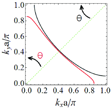
Figure 1: The Fermi surface of OP LSCO (black line) and OV LSCO (red line) given by Eq. (2). The OP and UD LSCO have an hole-like and OV LSCO has a electron-like Fermi surface, respectively, as can be seen from the figure. The tilt angle $\theta$ is given with respect to the nodal cut centered at $(\pi,\pi)$ for OP and UD, and at $(0,0)$ for OV LSCO.

The $4\times 4$ matrix self-energy may be written as[14]

$$\hat{\Sigma}(\mathbf{k},\omega)=\widetilde{\Sigma}(\mathbf{k},\omega)\tau_{0}+X(\mathbf{k},\omega)\tau_{3}+\phi(\mathbf{k},\omega)\tau_{2}\sigma_{2},$$ (7)

where $\tau_{i}$ and $\sigma_{i}$ are the Pauli matrices in the particle-hole and spin space, respectively. The diagonal self-energy is given by

$$\Sigma(\mathbf{k},\omega)=\widetilde{\Sigma}(\mathbf{k},\omega)+X(\mathbf{k},\omega),$$ (8)

and the diagonal spectral function measured by the ARPES is

$$A(\mathbf{k},\omega)=A_{S}(\mathbf{k},\omega)+A_{X}(\mathbf{k},\omega).$$ (9)

The symmetry of the self-energy is as follows.

$$\widetilde{\Sigma}(\mathbf{k},\omega) = -\widetilde{\Sigma}^{*}(\mathbf{k},-\omega),$$

$$X(\mathbf{k},\omega) = X^{*}(\mathbf{k},-\omega),$$

$$\phi(\mathbf{k},\omega) = \phi^{*}(\mathbf{k},-\omega).$$ (10)

We choose the following tight-binding band as the bare dispersion for the doped La_2-xSr_xCuO₄.[15]

$$\xi(\mathbf{k})=-2t(\cos k_{x}a+\cos k_{y}a)+4t^{\prime}\cos k_{x}a\cos k_{y}a$$

$$-2t^{\prime\prime}(\cos 2k_{x}a+\cos 2k_{y}a)-\mu.$$ (11)

The tight-binding parameters are $t=0.25$ eV, $t^{\prime}=0.15~{}t$, $t^{\prime\prime}=0.5~{}t^{\prime}$, and the chemical potential $\mu=-0.19$ eV for OP, and $t=0.25$ eV, $t^{\prime}=0.13~{}t$, $t^{\prime\prime}=0.5~{}t^{\prime}$, $\mu=-0.22$ eV for OV, and $t=0.25$ eV, $t^{\prime}=0.17~{}t$, $t^{\prime\prime}=0.5~{}t^{\prime}$, $\mu=-0.15$ eV for UD La_2-xSr_xCuO₄. The UD and OP La_2-xSr_xCuO₄ have a hole-like and OV has an electron-like FS as shown in Fig. 1. To denote the momentum direction in the BZ in two dimensions we use the tilt angle $\theta$ with respect to the nodal cut, that is, the diagonal cut along $(0,0)-(\pi,\pi)$ line, centered at $(\pi,\pi)$ for the hole like FS and at (0,0) for electron like FS as indicated in Fig. 1.

The spin fluctuation mechanism in this formulation means that we take $F_{ch}({\bf q},\omega)=0$ and $F_{sp}({\bf q},\omega)$ as the spin susceptibility $\chi_{sp}({\bf q},\omega)$ measured by INS in Eq. (2). Then the imaginary parts of the self-energy may be rewritten from Eq. (2) as

$$Im\widetilde{\Sigma}(\mathbf{k},\omega)=\pi\int^{\infty}_{-\infty}d\epsilon^{\prime}\left[f(\omega-\epsilon^{\prime})+n(-\epsilon^{\prime})\right]\sum_{\mathbf{k^{\prime}}}A_{S}(\mathbf{k^{\prime}},\omega-\epsilon^{\prime})\alpha^{2}\chi_{sp}(\mathbf{k}-\mathbf{k^{\prime}},\epsilon^{\prime}),$$

$$ImX(\mathbf{k},\omega)=\pi\int^{\infty}_{-\infty}d\epsilon^{\prime}\left[f(\omega-\epsilon^{\prime})+n(-\epsilon^{\prime})\right]\sum_{\mathbf{k^{\prime}}}A_{X}(\mathbf{k^{\prime}},\omega-\epsilon^{\prime})\alpha^{2}\chi_{sp}(\mathbf{k}-\mathbf{k^{\prime}},\epsilon^{\prime}),$$

$$Im\phi(\mathbf{k},\omega)=\pi\int^{\infty}_{-\infty}d\epsilon^{\prime}\left[f(\omega-\epsilon^{\prime})+n(-\epsilon^{\prime})\right]\sum_{\mathbf{k^{\prime}}}A_{\phi}(\mathbf{k^{\prime}},\omega-\epsilon^{\prime})\alpha^{2}\chi_{sp}(\mathbf{k}-\mathbf{k^{\prime}},\epsilon^{\prime}).$$ (12)

The real parts were calculated from the imaginary parts using the Kramers-Kronig (KK) relation. Eqs. (2) and (2) were solved self-consistently via iterations.

The coupling strength $\alpha$ was chosen such that it reproduces the experimentally measured gap amplitude $\Delta_{0}$ of La_2-xSr_xCuO₄.[16] The coupling strength will be given in terms of the dimensionless coupling constant $\lambda$ below,

$$\lambda=\int_{-\infty}^{\infty}d\omega N(\omega)\frac{\alpha^{2}\chi_{sp}(\omega)}{\omega},$$ (13)

where $N(\omega)$ is the density of states (DOS) and $\chi_{sp}(\omega)$ is the local spin susceptibility given by

$$\chi_{sp}(\omega)=\frac{\int d{\bf q}\ \chi_{sp}({\bf q},\omega)}{\int d{\bf q}}.$$ (14)

It is a measure of the density of spin excitation for a given energy. The gap function is determined by

$$\Delta(\mathbf{k})=Re\left[\frac{\phi(\mathbf{k},\omega)}{Z(\mathbf{k},\omega)}\right]_{\omega=\Delta(\mathbf{k})},$$ (15)

and $\Delta_{0}$ was determined from the DOS peak position.

The measured spin susceptibility $\chi_{sp}({\bf q},\omega)$ from INS was fitted by the form

$$\chi_{sp}({\bf q},\omega)=\chi_{\delta}(\omega)\frac{\kappa^{4}(\omega)}{\left[\kappa^{2}(\omega)+R({\bf q})\right]^{2}},$$

$$R({\bf q})=\frac{\left[(h-{\tfrac{1}{2}})^{2}+(k-\tfrac{1}{2})^{2}-\delta^{2}\right]^{2}+\lambda(h-\tfrac{1}{2})^{2}(k-\tfrac{1}{2})^{2}}{4\delta^{2}},$$ (16)

where the inplane wave-vector is written in the reciprocal lattice as ${\bf q}=h{\bf a}^{*}+k{\bf b}^{*}+l{\bf c}^{*}$, $\kappa(\omega)=1/\xi$ the inverse correlation length, the incommensurability $\delta(\omega)$ specifies the position of the four peaks, and $\lambda(\omega)$ controls the shape of the pattern. $\lambda$ = 4 corresponds to four distinct peaks and $\lambda$ = 0 corresponds to a pattern with circular symmetry. These fitting parameters were given in the references [8, 9, 10, 11]. Notice, however, that in these references the authors used the wave-vectors in the reciprocal lattice unit such that their 1/2, for example, corresponds to $\pi$ of this paper.

The measured local susceptibility may be decomposed into three parts; a low frequency incommensurate (IC) peak centered around ${\bf Q}_{\delta}=(\pi\pm\delta,\pi)$ and the symmetry related points, a commensurate (CM) peak at ${\bf Q}=(\pm\pi,\pm\pi)$, and a broad high frequency feature. The IC peak is around 18, 15, and 15 meV for OP, OV, and UD samples, respectively. The CM peak is around 50 meV for OP and 45 meV for UD samples, but is missing for OV La_2-xSr_xCuO₄. On the other hand, the high frequency feature persisting up to measurable energy is common for all samples. The cutoff energy $\omega_{c}$ of the susceptibility spectrum was taken to be 0.3 eV. This is the upper limit of the spin wave spectrum[17] of around $~{}2J$.

The $\mathbf{k}^{\prime}$ summation in Eq. (2) was performed by using the 2D fast Fourier transform (FFT) between the momentum and real space using the convolution relation

$$\sum_{\mathbf{k}}e^{i\mathbf{k}\cdot{\bf r}}\sum_{\mathbf{k}^{\prime}}F(\mathbf{k}^{\prime}-\mathbf{k})G(\mathbf{k}^{\prime})=F({\bf r})G({\bf r})$$ (17)

on a $2^{8}\times 2^{8}$ mesh of the first quadrant of BZ. No assumption about the $\mathbf{k}$ and $\omega$ dependence nor a separable form of the diagonal and off-diagonal self-energy was made in the calculations. Self-consistency is reached in a couple of tens of iterations.

3 Preliminary Analysis

Before presenting our results of the angle and frequency dependence of the self-energy, it will be useful to consider some simple cases. Let us first consider the Einstein model of frequency $\omega_{b}$ of the coupled boson.

$$\alpha^{2}F(\mathbf{k},\mathbf{k}^{\prime},\epsilon^{\prime})=\alpha^{2}(\mathbf{k},\mathbf{k}^{\prime})\left[\delta(\epsilon^{\prime}-\omega_{b})-\delta(\epsilon^{\prime}+\omega_{b})\right].$$ (18)

Then the imaginary part of the diagonal self-energy from Eq. (2) is

$$\Sigma_{2}(\mathbf{k},\omega)=\pi\left\{\left[f(\omega-\omega_{b})+n(-\omega_{b})\right]D(\mathbf{k},\omega-\omega_{b})\right.$$

$$\left.-\left[f(\omega+\omega_{b})+n(\omega_{b})\right]D(\mathbf{k},\omega+\omega_{b})\right\},$$ (19)

where

$$D(\mathbf{k},\omega)=\sum_{\mathbf{k}^{\prime}}\alpha^{2}(\mathbf{k},\mathbf{k}^{\prime})A(\mathbf{k}^{\prime},\omega).$$ (20)

In the low temperature limit of $T\rightarrow 0$, it is reduced to

$$-\Sigma_{2}(\mathbf{k},\omega)=\pi\left[\Theta(\omega-\omega_{b})D(\mathbf{k},\omega-\omega_{b})+\Theta(-\omega-\omega_{b})D(\mathbf{k},\omega+\omega_{b})\right],$$ (21)

where $\Theta$ is the step function. The peaks of $-\Sigma_{2}(\mathbf{k},\omega)$ for the negative (positive) $\omega$ region are determined by those of $D(\mathbf{k},\omega\pm\omega_{b})$. Depending on the range of $\mathbf{k}^{\prime}$ summation of Eq. (20) determined by $\alpha^{2}(\mathbf{k},\mathbf{k}^{\prime})$, either one peak (for $\kappa\rightarrow\infty$ or 0) or two peaks (for intermediate $\kappa$) may show up as discussed below.

Consider two limits of this expression: First, for momentum independent coupling of $\alpha^{2}(\mathbf{k},\mathbf{k}^{\prime})=\alpha^{2}$. Then, we have

$$-\Sigma_{2}(\mathbf{k},\omega)=\left\{\begin{array}[]{ll}\pi\alpha^{2}N(\omega-\omega_{b}),&{\rm for~{}}\omega>\omega_{b},\\ \pi\alpha^{2}N(\omega+\omega_{b}),&{\rm for~{}}\omega<-\omega_{b},\\ 0,&{\rm otherwise}.\end{array}\right.$$ (25)

where

$$N(\omega)=\sum_{\mathbf{k}^{\prime}}A(\mathbf{k}^{\prime},\omega)$$ (26)

is DOS. This clearly shows that the peaks of DOS at $\omega=\pm\Delta_{0}$ in the SC state are shifted to $\pm(\Delta_{0}+\omega_{b})$ in $-\Sigma_{2}(\omega)$ because of the coupling to the boson of frequency of $\omega_{b}$ and that they are momentum independent. This case is relevant where the correlation length $\xi$ of a susceptibility peak is small (or, the inverse correlation length $\kappa\rightarrow\infty$) like the 50 meV CM peak of OP sample. See the angle independent peaks near $|\omega|\approx 65$ meV in $-\Sigma_{2}$ and $\phi_{2}$ shown in Figs. 2(a) and 3(a).

Another limit is where the coupling is a delta function like $\alpha^{2}(\mathbf{k},\mathbf{k}^{\prime})=\alpha^{2}~{}\delta(\mathbf{k}^{\prime}-\mathbf{k}-{\bf q})$, corresponding to $\kappa\rightarrow 0$. Then, instead of Eq. (25), we have

$$-\Sigma_{2}(\mathbf{k},\omega)=\left\{\begin{array}[]{ll}\pi\alpha^{2}A(\mathbf{k}+{\bf q},\omega-\omega_{b}),&{\rm for~{}}\omega>\omega_{b},\\ \pi\alpha^{2}A(\mathbf{k}+{\bf q},\omega+\omega_{b}),&{\rm for~{}}\omega<-\omega_{b},\\ 0,&{\rm otherwise}.\end{array}\right.$$ (30)

Because the spectral function $A(\mathbf{k},\omega)$ has a peak around $\omega\approx\pm E(\mathbf{k})$ in SC state, where

$$E(\mathbf{k})=\sqrt{\widetilde{\xi}^{2}(\mathbf{k})+\Delta^{2}(\mathbf{k})},$$ (31)

and $\widetilde{\xi}(\mathbf{k})=(\xi(\mathbf{k})+X)/Z$ is the renormalized dispersion, the peak of $-\Sigma_{2}(\mathbf{k},\omega)$ occurs at $\omega\approx\pm(E(\mathbf{k}+{\bf q})+\omega_{b})$ which is clearly momentum and band structure dependent.

For intermediate values of $\kappa$, the self-energy of Eq. (30) is summed around $\mathbf{k}+{\bf q}$ over the width $~{}\kappa$. Then, both energy scales of $(\Delta_{0}+\omega_{b})$ and $(E(\mathbf{k}+{\bf q})+\omega_{b})$ may appear in $-\Sigma_{2}(\mathbf{k},\omega)$ from a single peak of $\chi({\bf q},\omega)$. A modification is that the energy $(\Delta_{0}+\omega_{b})$ of $\xi\rightarrow 0$ now becomes momentum dependent $(\Delta^{\prime}(\mathbf{k})+\omega_{b})$ because a non-zero $\xi$ implies a momentum selection in the $\mathbf{k}^{\prime}$ summation. $\Delta^{\prime}(\mathbf{k})$ is an angle dependent energy of order $\Delta_{0}$. This seems to be the case for the IC peaks as will be discussed below.

Some complications arise from the band structure and momentum dependent coupling.[12] An interesting case is where the momentum sum covers the saddle point which usually occurs at $(0,\pi)$. This introduces another energy scale in $-\Sigma_{2}(\mathbf{k},\omega)$ from the van Hove singularity (VHS). It occurs at $\omega\approx sgn(\xi_{VHS})(E_{VHS}+\omega_{b})$, where $E_{VHS}=\sqrt{\widetilde{\xi}^{2}(0,\pi)+\Delta_{0}^{2}}$ and $sgn(f)=\pm 1$ represents the sign of $f$, in addition to the two energy scales of the peaks discussed above. The shape of $\Sigma(\mathbf{k},\omega)$ are also modified by the impurity scatterings.[18] The VHS peak may be substantially suppressed by the coupling to boson spectrum and impurity scatterings. One should perform the self-consistent calculations to see their effects without misleading conclusion. The off-plane elastic impurities may induce interesting features of the self-energy in the SC state.

In cases where the VHS peak is strongly suppressed and/or the $E_{VHS}$ and $\Delta_{0}$ are not well separated, the VHS feature may not clearly show up. The parameters of current LSCO calculations seem to belong to this case and we do not discuss the VHS features in the self-energy below. Also recall that the discussion so far is restricted to a sharp boson frequency of a single energy. A finite width in energy as well as in momentum space smoothens peak features in the self-energy.

4 Numerical Results

We now turn to the self-consistent numerical calculations using the experimentally measured spin susceptibility as the Eliahberg function for the OP, OV, and UD La_2-xSr_xCuO₄ as explained above. The angle $\theta$ in the BZ was chosen with respect to the nodal direction as shown in Fig. 1. We wish to discuss the position and intensity of peaks in the absolute value of the imaginary part, $-\Sigma_{2}(\mathbf{k},\omega)$, and the real part of the self-energy, $\Sigma_{1}(\mathbf{k},\omega)$, for $\omega<0$. The $\omega>0$ region can not be probed by the ARPES with which we wish to compare our numerical results. For the off-diagonal self-energy, $\phi_{1}(\mathbf{k},\omega)$ and $\phi_{2}(\mathbf{k},\omega)$ are, respectively, even and odd functions of $\omega$, and will be shown in the $\omega>0$ region.

4.1 OP La_2-xSr_xCuO₄

First, we consider the OP La_2-xSr_xCuO₄ with the doping concentration $x=0.16$ and the critical temperature $T_{c}=38.5$ K. The spin susceptibility spectrum reported by Vignolle $et~{}al.$ has three parts; the IC peak near 18 meV, CM peak near 50 meV, and broad high frequency feature extended to 0.3 eV. The coupling constant was chosen such that $\lambda=1.74$ in the calculations to obtain the gap amplitude $\Delta_{0}=17$ meV in the $T\rightarrow 0$ limit.[16]

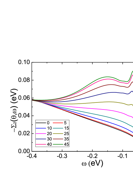
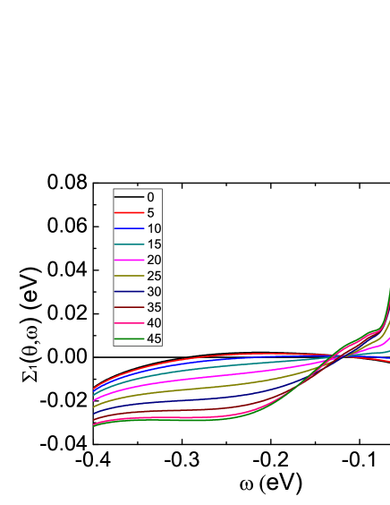
Figure 2: The calculated imaginary and real parts of the diagonal self-energy at the Fermi momentum of OP LSCO along several cuts in BZ in the SC state. The Vignolle spectrum was used for the $F_{sp}$ in the Eliashberg equation. The nodal direction is 0 deg and the anti-nodal direction is 45 deg.

Fig. 2(a) and (b) are the imaginary and real parts of the diagonal self-energy along several cuts perpendicular to the FS in the BZ in SC state. Fig. 3(a) and (b) show the imaginary and real parts of the off-diagonal self-energy, respectively. The two peaks in both the real and imaginary parts of the diagonal and off-diagonal self-energies reflect the two peaks in the spin susceptibility with slight complication as explained below.

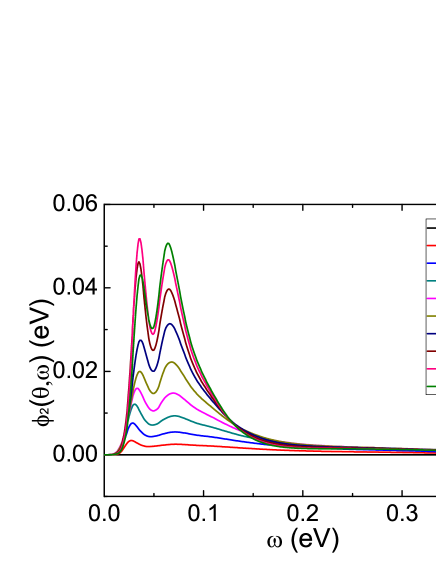
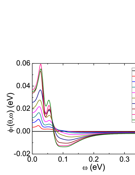
Figure 3: The calculated imaginary and real parts of the off-diagoanl self-energy of OP LSCO along several cuts perpedicular to the FS in the SC state. The angles are the same as the Fig. 2.

For the Vignolle spectrum from OP La_2-xSr_xCuO₄, the IC peak has an intermediate correlation length of $\xi\approx 4.1a$, the CM peak has a small $\xi\approx 0.8a$, and the broad high frequency feature has $\xi\approx 0.7a$.[8] From the discussion in the previous section, we may expect two peaks at $\omega_{1}\approx-(\Delta^{\prime}(\mathbf{k})+\omega_{IC})$ and $\omega^{\prime}_{1}\approx-(E(\mathbf{k}+{\bf Q_{\delta}})+\omega_{IC})$ from the IC peak, and one peak at $\omega_{2}\approx-(\Delta_{0}+\omega_{CM})$ from CM peak. The $\omega^{\prime}_{1}$ seems to overlap with $\omega_{2}$, and two peaks show up in $-\Sigma_{2}(\mathbf{k},\omega)$. The $\omega_{1}$ is expected to be angle-dependent and $\omega_{2}$ to be $\approx-67$ meV because $\Delta_{0}=17$ and $\omega_{CM}\approx 50$ meV. This is what we obtained in numerical calculations as shown in Fig. 2(a). The exactly same argument holds for the off-diagonal self-energy, $\phi_{2}(\mathbf{k},\omega)$ as shown in Fig. 3(a).

In order to understand the peak energy of the real parts of the self-energy, recall that the real and imaginary parts are related by the KK relation. It means that the peak energy of $\Sigma_{1}(\omega)$ is shifted from that of $-\Sigma_{2}(\omega)$ by the width of the peak, that is, the peak energy of $\Sigma_{1}$ is expected at $\omega\approx-(\Delta^{\prime}(\mathbf{k})+\omega_{IC}-\Gamma_{IC})$ and $\omega\approx-(\Delta_{0}+\omega_{CM}-\Gamma_{CM})$, where $\Gamma$ is the width of the peak. This is indeed what we obtained from numerical calculations. See the plots of $\Sigma_{1}(\mathbf{k},\omega)$ and $\phi_{1}(\mathbf{k},\omega)$ as shown in Figs. 2(b) and 3(b), respectively.

Now, we turn to the intensity of the peaks of the self-energy. From Eqs. (21) and (20) we see that $-\Sigma_{2}(\mathbf{k},\omega)$ is given by the sum over $\mathbf{k}^{\prime}$ of $\alpha^{2}(\mathbf{k},\mathbf{k}^{\prime})A(\mathbf{k}^{\prime},\omega+\omega_{b})$. It means that there is large contribution from the $\mathbf{k}^{\prime}$ sum to $-\Sigma_{2}(\mathbf{k},\omega)$ if both $\mathbf{k}^{\prime}-\mathbf{k}\approx{\bf Q}_{\delta}$ and $\omega\approx-(E(\mathbf{k}+{\bf Q}_{\delta})+\omega_{IC})$ are satisfied. This is better satisfied near the anti-nodal region and $-\Sigma_{2}(\mathbf{k},\omega)$ increases as the tilt angle increases for small $|\omega|$. For large $|\omega|$, however, either of the two conditions become ill satisfied and $-\Sigma_{2}(\mathbf{k},\omega)$ is roughly angle independent. This is indeed what Fig. 2(a) shows. The IC peak in all four plots in Fig. 2 and Fig. 3 is not highest at 45 deg but $\approx 40$ deg because of the incommensurability $\delta$. On the other hand, the CM peak near 65 meV is highest at 45 deg as expected because the broad CM peak connects the anti-nodal regions most effectively.

The angle dependence of the off-diagonal self-energy $\phi(\theta,\omega)$ along several cuts is roughly $d$-wave like as shown in Fig. 3. The imaginary part looks like the local spin susceptibility $\chi_{sp}(\omega)$ with the suppressed high frequency part. The suppression of $\phi_{2}(\theta,\omega)$ above $\sim 0.1$ eV shows that the high frequency part of the susceptibility does not contribute much to pairing because its broad momentum dependence is not very effective for $d$-wave pairing. The real part $\phi_{1}(\theta,\omega)$ increases as $\omega$ increases from 0 and exhibits two peaks induced by the two peaks in the spin susceptibility and then decreases and makes a zero crossing near $\omega_{2}$. There, $\phi_{2}(\theta,\omega)$ has a peak because of the KK relation.

4.2 OV La_2-xSr_xCuO₄

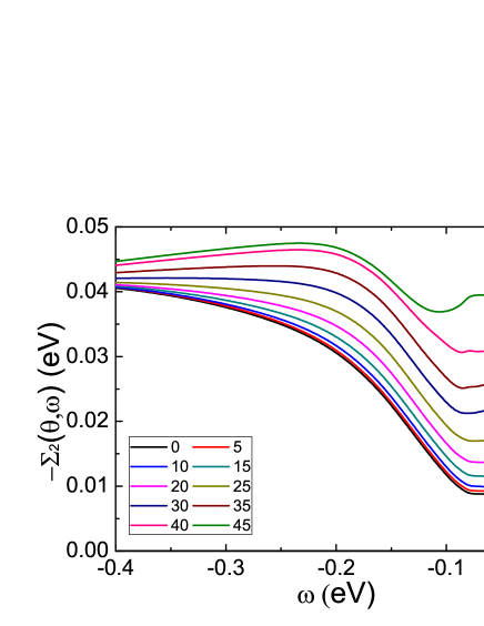
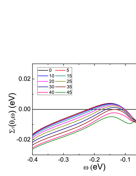
Figure 4: The calculated imaginary and real parts of the diagonal self-energy of OV LSCO along several cuts in BZ in the SC state.

The calculations were done for OV La_2-xSr_xCuO₄ as well. The difference from the OP case is that (a) the spin susceptibility spectrum does not have the CM component, and (b) the bare dispersion has smaller next nearest neighbor hopping amplitude of $t^{\prime}/t=0.13$ and has an electron-like FS. The IC peak at 15 meV of the spin suscetibility has the correlation length of $\xi\approx 2.7a$ and the broad high energy feature has $\xi\approx 0.6a$.[10] The coupling constant was chosen such that $\lambda=1.98$ to obtain the gap amplitude $\Delta_{0}=11$ meV at $T=0$ in calculations.

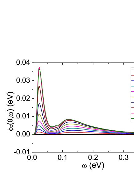
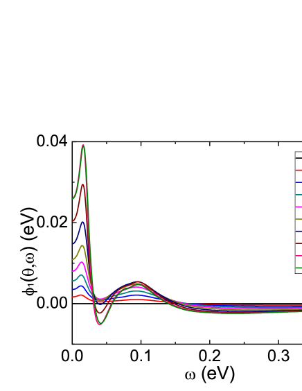
Figure 5: The calculated imaginary and real parts of the off-diagoanl self-energy at the Fermi momentum of OV LSCO in the SC state.

Fig. 4(a) and (b) are the imaginary and real parts of the diagonal self-energy along several cuts perpendicular to the Fermi surface in the BZ. The results may be understood like the OP case. The single IC peak in the spin susceptibility has an intermediate correlation length and induces two peaks in $-\Sigma_{2}(\mathbf{k},\omega)$. Because the correlation length is rather small, the angle dependence of the peak at $\omega_{1}\approx-25$ and $\omega_{2}\approx-75$ meV are weak. The peak at $\omega_{1}$ is the shift of the DOS peak because $\Delta_{0}+\omega_{IC}\approx 26$ meV. The peak at $\omega_{2}$ is from the $-(E(\mathbf{k}+{\bf Q}_{\delta})+\omega_{IC})$ as was discussed in the OP case. We note that the VHS peak can not appear in the negative energy because OV LSCO has electron-like Fermi surface.

Fig. 5(a) and (b) show the imaginary and real parts of the off-diagonal self-energy along several cuts in BZ. The angle dependence is roughly $d$-wave like. The imaginary part of the off-diagonal self-energy $\phi_{2}(\theta,\omega)$ has a peak near $\omega_{1}\approx 25$ meV and looks like the local spin susceptibility with the suppressed high frequency part as the OP case. The real part $\phi_{1}(\theta,\omega)$ begins to increase as $\omega$ increases from 0, has a peak and then decreases and makes a zero-crossing near $\omega_{1}$ where the $\phi_{2}(\theta,\omega)$ has the IC peak.

4.3 UD La_2-xSr_xCuO₄

The calculations were done for UD La_2-xSr_xCuO₄ as well. The spin susceptibility spectrum reported by Lipscombe $et~{}al.$[10, 11] for 8% doping La_2-xSr_xCuO₄ was used in the calculations. The spectrum $\chi_{sp}(\omega)$ has three parts as the OP case; the IC peak near 15 meV, CM peak near 45 meV, and a broad high frequency feature extrapolated upto 0.38 eV. The IC and CM peaks have the correlation lengths of $\xi\approx 2.45a$ and $0.8a$, respectively.[11] The coupling constant was chosen such that $\lambda=1.58$ to obtain the gap amplitude $\Delta_{0}=17$ meV at $T=0$ in the calculations.[16]

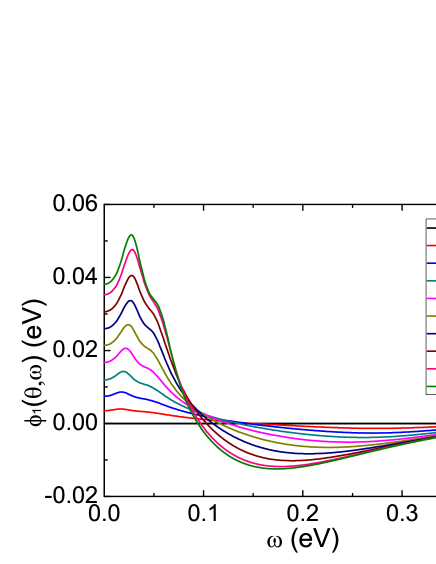
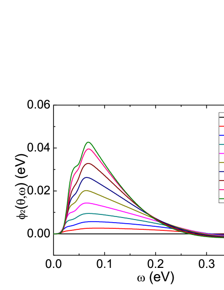
Figure 6: (a), (b) The calculated imaginary and real parts of the diagonal self-energy of UD LSCO along several cuts in BZ in the SC state.

Fig. 6(a) and (b) are the imaginary and real parts of the diagonal self-energy along several cuts perpendicular to the Fermi surface in the BZ. The results may be understood like the OP and OV cases. Because the peaks of the susceptibility are broader in frequency than OP and OV materials, the peaks in the self-energy are not as sharp as the OP and OV cases.

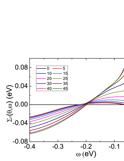
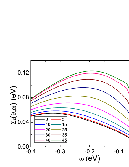
Figure 7: (a), (b) The calculated imaginary and real parts of the off-diagoanl self-energy.

Fig. 7(a) and (b) show the imaginary and real parts of the off-diagonal self-energy along several cuts. The angle dependence is roughly $d$-wave like. The two peaks in the diagonal and off-diagonal self-energy are from the IC and CM peaks of the spin susceptibility. Their energy in the imaginary parts is expected at $\omega_{1}\approx\Delta_{0}+\omega_{IC}\approx 32$ and $\omega_{2}\approx\Delta_{0}+\omega_{CM}\approx 62$ meV. The peaks in the real parts are shifted by the width. This is what we obtained from the calculations as shown in Figs. 6 and 7.

5 Summary  and  Concluding Remarks

We have calculated the full momentum and frequency dependence of the self-energy by solving the Eliashberg equation using the measured spin susceptibility from inelastic neutron scattering experiments on optimally, overdoped, and underdoped La_2-xSr_xCuO₄ cuprates in the SC state. The real and imaginary parts of the diagonal and off-diagonal self-energy were presented for several cuts perpendicular to the Fermi surface for each doping concentration.

The results of calculations were discussed in terms of the angle (i.e. the direction of momentum in the BZ) dependence of the peak position and intensity. First, the angle dependence of the peak intensity is that the spin fluctuation induced self-energy $\Sigma(\mathbf{k},\omega)$ is very anisotropic in the momentum space for small $|\omega|$. We can see from Fig. 2(a) that the absolute value of the imaginary part of the diagonal self-energy of OP LSCO increases by a factor of about 5 from nodal to anti-nodal directions below the CM peak of $|\omega|\leq 70$ meV. The real part also changes roughly by the same factor as can be seen from the inset of Fig. 2(b). This is understandable because the spin susceptibility with the correlation length $\xi\approx 4.1a$ must mean that the quasi-particle dynamics is very different for different directions in the BZ. Second, The angle dependence of the peak position is that the CM peak is angle independent at around $|\omega_{2}|\approx 70$ meV and the IC peak position $|\omega_{1}|$ increases from $\approx 25$ to 37 meV as the angle changes from the nodal to antinodal direction for OP LSCO.

As alluded in the introduction, this angle dependence of the peak energy may not be properly addressed in the approaches where a separable form of the off-diagonal self energy like $\phi(\mathbf{k},\omega)=\phi(\omega)[\cos(k_{x}a)-\cos(k_{y}a)]$ or $\phi(\mathbf{k},\omega)=\phi(\omega)\cos(2\theta)$,[12, 7, 4] or a phenomenological form of the spin susceptibility is assumed. For example, the separable form of the off-diagonal self-energy may give misleading results with regard to the angle dependence of an energy scale because the angle dependence was built in by hands. No such assumptions were made in this work.

The present results may be checked against the proposed spin fluctuation theory for the cuprate superconductivity. The most direct evidence of the spin fluctuation theory will be to detect the angle and frequency dependence of the diagonal and off-diagonal self-energy experimentally and compare it with the results presented here. This will be an extension of the McMillan-Rowell procedure of phonon superconductors[19] to $d$-wave pairing. The experiment of choice for this purpose will be the ARPES because of its high momentum and frequency resolution capability.

Indeed, the self-energy has been deduced by performing the momentum distribution curve analysis of the ARPES intensity for Bi₂Sr₂CaCu₂O_8+δ. For La_2-xSr_xCuO₄ crystals high quality ARPES data are not available for comparison though. The requirement of high resolution ARPES intensity data is being met only recently for Bi₂Sr₂CaCu₂O_8+δ using the Laser ARPES.[20, 13, 21]

If we compare the present calculations on LSCO with the ARPES analysis from BSCO, bearing the difference in mind, we notice that the peak intensity of the real part of the self-energy from BSCO does not change so much as the present calculations. From the nodal ($\theta=0$) to 30 deg, the peak height changes by less than a factor of 1.5. The angle dependence of the peak position is different too. From nodal to anti-nodal direction the peak position decreases in contrary to the present calculations based on the AF fluctuations.[13, 21] Proper comparison, of course, must await high resolution ARPES data from La_2-xSr_xCuO₄ materials which may be quantitatively checked against the present calculations.

We wish to thank Stephen Hayden for sending us the Ref. [11] and Chandra Varma for useful comments on the manuscript. This work was supported by National Research Foundation (NRF) of Korea through Grant No. NRF 2010-0010772.

References

- [1] D. J. Scalapino. A common thread: The pairing interaction for unconventional superconductors. Rev. Mod. Phys., 84:1383–1417, Oct 2012.
- [2] P. Monthoux, D. Pines, and G. G. Lonzarich. Superconductivity without phonons. Nature, 450(7173):1177–1183, 2007.
- [3] M. R. Norman. High temperature superconductivity - magnetic mechanisms. 2006.
- [4] T. Dahm, V. Hinkov, S. V. Borisenko, A. A. Kordyuk, V. B. Zabolotnyy, J. Fink, B. Buchner, D. J. Scalapino, W. Hanke, and B. Keimer. Strength of the spin-fluctuation-mediated pairing interaction in a high-temperature superconductor. Nature Phys., 5:217, 2009.
- [5] Philip W. Anderson. Is there glue in cuprate superconductors? Science, 316:1705–1707, 2007.
- [6] T. A. Maier, D. Poilblanc, and D. J. Scalapino. Dynamics of the pairing interaction in the hubbard and models of high-temperature superconductors. Phys. Rev. Lett., 100:237001, Jun 2008.
- [7] A. J. Millis. Nearly antiferromagnetic fermi liquids: An analytic eliashberg approach. Phys. Rev. B, 45:13047–13054, Jun 1992.
- [8] B. Vignolle, S. M. Hayden, D. F. McMorrow, H. M. Ronnow, B. Lake, C. D. Frost, and T. G. Perring. Two energy scales in the spin excitations of the high-temperature superconductor la2-xsrxcuo4. Nature Phys., 3:163–167, 2007.
- [9] O. J. Lipscombe, S. M. Hayden, B. Vignolle, D. F. McMorrow, and T. G. Perring. Persistence of high-frequency spin fluctuations in overdoped superconducting (). Phys. Rev. Lett., 99:067002, Aug 2007.
- [10] O. J. Lipscombe, B. Vignolle, T. G. Perring, C. D. Frost, and S. M. Hayden. Emergence of coherent magnetic excitations in the high temperature underdoped superconductor at low temperatures. Phys. Rev. Lett., 102:167002, Apr 2009.
- [11] Oliver Jon Lipscombe. High-Energy Spin Fluctuations in the Cuprate Superconductors. PhD thesis, University of Bristol, May 2008.
- [12] A. W. Sandvik, D. J. Scalapino, and N. E. Bickers. Effect of an electron-phonon interaction on the one-electron spectral weight of a d-wave superconductor. Phys. Rev. B, 69:094523, Mar 2004.
- [13] Jae Hyun Yun, Jin Mo Bok, Han-Yong Choi, Wentao Zhang, X. J. Zhou, and Chandra M. Varma. Analysis of laser angle-resolved photoemission spectra of ba2sr2cacu2o8+δ in the superconducting state: Angle-resolved self-energy and the fluctuation spectrum. Phys. Rev. B, 84:104521, 2011.
- [14] K. Maki. Gapless superconductivity. In R. D. Parks, editor, Superconductivity, Vol. 2, pages 1035–1106. Marcel Dekker, New York, 1969.
- [15] T. Yoshida, X. J. Zhou, K. Tanaka, W. L. Yang, Z. Hussain, Z.-X. Shen, A. Fujimori, S. Sahrakorpi, M. Lindroos, R. S. Markiewicz, A. Bansil, Seiki Komiya, Yoichi Ando, H. Eisaki, T. Kakeshita, and S. Uchida. Systematic doping evolution of the underlying fermi surface of . Phys. Rev. B, 74:224510, Dec 2006.
- [16] Teppei Yoshida, Makoto Hashimoto, Inna M. Vishik, Zhi-Xun Shen, and Atsushi Fujimori. Pseudogap, superconducting gap, and fermi arc in high- cuprates revealed by angle-resolved photoemission spectroscopy. J. Phys. Soc. Jap., 81(1):011006, 2012.
- [17] N. S. Headings, S. M. Hayden, R. Coldea, and T. G. Perring. Anomalous high-energy spin excitations in the high- superconductor-parent antiferromagnet . Phys. Rev. Lett., 105:247001, Dec 2010.
- [18] L. Zhu, P. J. Hirschfeld, and D. J. Scalapino. Elastic forward scattering in the cuprate superconducting state. Phys. Rev. B, 70:214503, Dec 2004.
- [19] W. L. McMillan and J. M. Rowell. Lead phonon spectrum calculated from superconducting density of states. Phys. Rev. Lett., 14(4):108–112, Jan 1965.
- [20] Wentao Zhang, Jin Mo Bok, Jae Hyun Yun, Junfeng He, Guodong Liu, Lin Zhao, Haiyun Liu, Jianqiao Meng, Xiaowen Jia, Yingying Peng, Daixiang Mou, Shanyu Liu, Li Yu, Shaolong He, Xiaoli Dong, Jun Zhang, J. S. Wen, Z. J. Xu, G. D. Gu, Guiling Wang, Yong Zhu, Xiaoyang Wang, Qinjun Peng, Zhimin Wang, Shenjin Zhang, Feng Yang, Chuangtian Chen, Zuyan Xu, H.-Y. Choi, C. M. Varma, and X. J. Zhou. Extraction of normal electron self-energy and pairing self-energy in the superconducting state of the bi2sr2cacu2o8 superconductor via laser-based angle-resolved photoemission. Phys. Rev. B, 85:064514, Feb 2012.
- [21] J. He, W. Zhang, J. M. Bok, D. Mou, L. Zhao, Y. Peng, S. He, G. Liu, X. Dong, J. Zhang, J. S. Wen, Z. J. Xu, G. D. Gu, X. Wang, Q. Peng, Z. Wang, S. Zhang, F. Yang, C. Chen, Z. Xu, H.-Y. Choi, C. M. Varma, and X. J. Zhou. Coexistence of Two Sharp-Mode Couplings and Their Unusual Momentum Dependence in the Superconducting State of Bi2Sr2CaCu2O8+d Superconductor Revealed by Laser-Based Angle-Resolved Photoemission. ArXiv e-prints, October 2012.