A Multiobjective State Transition Algorithm for Single Machine Scheduling

Abstract

In this paper, a discrete state transition algorithm is introduced to solve a multiobjective single machine job shop scheduling problem. In the proposed approach, a non-dominated sort technique is used to select the best from a candidate state set, and a Pareto archived strategy is adopted to keep all the non-dominated solutions. Compared with the enumeration and other heuristics, experimental results have demonstrated the effectiveness of the multiobjective state transition algorithm.

1 Introduction

The multiobjective optimization is encountered in many real world applications [1]. For a specific policy, the decision maker may find it advantageous for one goal but disadvantageous for others. A traditional way to deal with this issue is to impose a priori preference reflecting the relative importance of different objectives; however, the final solution just indicates a decision maker’s satisfaction, and it might be dissatisfactory for other decision makers.

To ameliorate the problem, the concept of Pareto optimality and other relevant concepts are introduced. These are defined as follows:

1) Pareto dominance: A feasible solution $\bm{x}=(x_{1},\cdots,x_{n})$ is said to Pareto dominate another feasible solution $\bm{y}=(y_{1},\cdots,y_{n})$, denoted as $\bm{x}\prec\bm{y}$, if

$$f_{i}(\bm{x})\leq f_{i}(\bm{y}),\forall i\in\{1,\cdots,k\},\;\mathrm{and}\;\;\exists j\in\{1,\cdots,k\},f_{j}(\bm{x})<f_{j}(\bm{y}),$$ (1)

where, $f_{i}(\bm{x})$ is the $i$th objective function, $k$ is the number of objectives.

2) Pareto optimality: A feasible solution $\bm{x}^{*}$ is said to be Pareto optimal if and only if

$$\neg\exists\bm{x}\in S,\bm{x}\prec\bm{x}^{*},$$ (2)

where, $S$ is the feasible space.

3) Pareto optimal set: The Pareto optimal set, denoted as $P^{*}$, is defined by

$$P^{*}=\{\bm{x}^{*}\in S|\neg\exists\bm{x}\in S,\bm{x}\prec\bm{x}^{*}\}.$$ (3)

4) Pareto front: The Pareto front, denoted as $Pf^{*}$, is defined by

$$Pf^{*}=\{(f_{1}(\bm{x}^{*}),\cdots,f_{k}(\bm{x}^{*}))|\bm{x}^{*}\in P^{*}\}.$$ (4)

The introduction of Pareto optimality allows us to find a set of Pareto optimal solutions simultaneously, independent of the decision maker’s priori preference.

In the past few decades, evolutionary-based and nature-inspired multiobjective optimization techniques have drawn considerable attention for scheduling problems[2, 3, 4, 5, 6, 7]. In this paper, we introduce a recently new heuristics called state transition algorithm [8, 9, 10, 11] as the basic search engine for the multiobjective optimization. A non-dominated sort approach is used to select the best from a candidate state set, and the best state is stored using a Pareto archive strategy. Experimental results have testified the effectiveness of the proposed algorithm.

2 Problem Description

In the field of joinery manufacturing, jobs with similar materials can be scheduled together to minimize the amount of materials used; therefore, reducing the cost.

For example, based on the cost savings matrix shown in Table 1, pairing Job1 and Job2 will provide saving in the cost equivalent to 4 units.

Table 1: The cost savings matrix for 5 jobs having the same material

	Job1	Job2	Job3	Job4	Job5
Job1	0	4	2.64	4.08	3.9
Job2	4	0	3.64	4.72	4.23
Job3	2.64	3.64	0	2.65	2.87
Job4	4.08	4.72	2.65	0	3.84
Job5	3.9	4.23	2.87	3.84	0

Additionally, based on the jobs’ processing times and due dates as shown in Table 2, and for any given sequence and pairing of jobs, not only the total cost saving C is affected but also the total tardiness time T, which is calculated as:

$$T=\sum_{j=1}^{n}\max\{0,c_{j}-d_{j}\}$$ (5)

where, $c_{j}$ and $d_{j}$ are the completion time and the due time of job $j$, respectively.

Table 2: Due dates and processing times for a set of 5 jobs

Job	Due Date(days)	Processing Time(hours)
Job1	8	17:40
Job2	2	24:00
Job3	11	19:20
Job4	3	25:00
Job5	3	14:40

• Number of operational hours = 8 hours per day

The goal of this paper is to determine the optimal sequence with pairing, in order to maximize the total cost savings and minimize the total tardiness time.

It is obvious that finding the permutation of the sequence $\{1,2,\cdots,n\}$ with pairing becomes a solution to the multiobjective single machine scheduling problem; however, not without the necessity to discuss the number of pairs for any fixed sequence of jobs.

Given a sequence $s=(1,2,\cdots,n)$, for $n=3$, we have 2 possible pairing options (1-2)-3 and 1-(2-3); for $n=4$, we have 2 possible pairing options (1-2)-(3-4) and 1-(2-3)-4, as pairing options (1-2)-3-4 and 1-2-(3-4) are discarded; for $n=5$, we have 3 possible options (1-2)-(3-4)-5, (1-2)-3-(4-5) and 1-(2-3)-(4-5), as options (1-2)-3-4-5, 1-2-(3-4)-5, 1-2-3-(4-5) and 1-(2-3)-4-5 are discarded.

If $P1(n)$ denotes the number of pairs with the first two jobs pairing, and $P2(n)$ denotes the complement of $P1(n)$, then we have the following theorem:
Theorem 1

$$P1(n+1)=P(n-1),P2(n+1)=P1(n),n\geq 3$$ (6)

where, $P(n)=P1(n)+P2(n)$ is the total number of pairs. For example, $P1(2)=1,P2(2)=0$, $P1(3)=1,P2(3)=1$, $P1(4)=1,P2(4)=1$, $P1(5)=2,P2(5)=1$, we have $P1(4)=P(2),P2(4)=P1(3)$, $P1(5)=P(3),P2(5)=P1(4)$.

Fig. 1, shows the growth trend of the number of pairs with the sequence size; however, only small size job scheduling problems are considered in this study. Considering that $P(10)=12\ll 10!=3628800$, a complete enumeration approach is used for pairing and only the permutation of a sequence is focused.

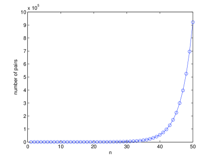
Figure 1: Growth trend relative to the sequence size

3 Discrete State Transition Algorithm

In the case a solution to a specific optimization problem is described as a state, then the transformation to update the solution becomes a state transition. Without loss of generality, the unified form of discrete state transition algorithm can be described as:

$$\left\{\begin{array}[]{ll}\bm{x}_{k+1}=A_{k}(\bm{x}_{k})\bigoplus B_{k}(\bm{u}_{k})\\ y_{k+1}=f(\bm{x}_{k+1})\end{array}\right.,$$ (9)

where, $\bm{x}_{k}\in\mathcal{Z}^{n}$ stands for a current state, corresponding to a solution of a specific optimization problem; $\bm{u}_{k}$ is a function of $\bm{x}_{k}$ and historical states; $A_{k}(\cdot)$, $B_{k}(\cdot)$ are transformation operators, which are usually state transition matrixes; $\bigoplus$ is an operation, which is admissible to operate on two states; and $f$ is the cost function or evaluation function.

The following three transformation operators are defined to permute current solution [10]:
(1) Swap Transformation

$$\bm{x}_{k+1}=A^{swap}_{k}(m_{a})\bm{x}_{k},$$ (10)

where, $A^{swap}_{k}\in\mathbb{R}^{n\times n}$ is the swap transformation matrix, $m_{a}$ is the swap factor, a constant integer used to control the maximum number of positions to be exchanged, while the positions are random. Fig. 2 shows an example of the swap transformation with $m_{a}=2$.

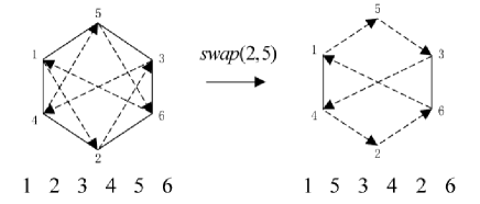
Figure 2: Illustration of the swap transformation

(2) Shift Transformation

$$\bm{x}_{k+1}=A^{shift}_{k}(m_{b})\bm{x}_{k},$$ (11)

where, $A^{shift}_{k}\in\mathbb{R}^{n\times n}$ is the shift transformation matrix, $m_{b}$ is the shift factor, a constant integer used to control the maximum length of consecutive positions to be shifted. Note that both the selected position to be shifted after and positions to be shifted are chosen randomly. Fig. 3 shows an example of the shift transformation with $m_{b}=1$.

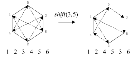
Figure 3: Illustration of the shift transformation

(3) Symmetry Transformation

$$\bm{x}_{k+1}=A^{sym}_{k}(m_{c})\bm{x}_{k},$$ (12)

where, $A^{sym}_{k}\in\mathbb{R}^{n\times n}$ is the symmetry transformation matrix, $m_{c}$ is the symmetry factor, a constant integer used to control the maximum length of subsequent positions as center. Note that both the component before the subsequent positions and consecutive positions to be symmetrized are created randomly. Fig. 4 shows an example of the symmetry transformation with $m_{c}=0$.

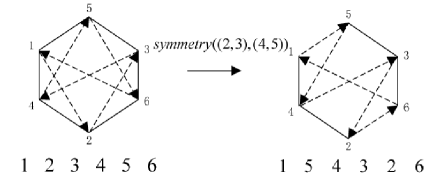
Figure 4: Illustration of symmetry transformation

4 Pareto Archived Strategy based on DSTA

In state transition algorithm, the times of transformation are called search enforcement (SE); as a result, after each transformation operator, a candidate state set $S$ is generated.

4.1 Non-dominated sort

We use a sorting approach similar to the fast-non-dominated-sort proposed in [12], described as follows:

1:for each $s\in S$ do

2:     $n_{s}\leftarrow 0$

3:     for each $t\in S$ do

4:         if $t\prec s$ then

5:              $n_{s}\leftarrow n_{s}+1$

6:         end if

7:     end for

8:end for

where, $n_{s}$ is the domination count, representing the number of solutions dominating solution $s$. After the non-dominated sort, the state with the least count will be stored as incumbent best for the next transformation operator.

4.2 Pareto Archived Strategy

We adopt a simple Pareto archived strategy to select current best, as follows:

1:for each $A_{i}\in\mathcal{A}$ do

2:     if $best\prec A_{i}$ then

3:         $\mathcal{A}\leftarrow\mathcal{A}-A_{i}$

4:     else if $A_{i}\prec best$ then

5:         $\mathcal{A}\leftarrow\mathcal{A}$

6:     else

7:         $\mathcal{A}\leftarrow\mathcal{A}\bigcup best$

8:     end if

9:end for

where, $\mathcal{A}$ is the archive keeping all non-donominated solutions.

4.3 Pseudocodes of the proposed algorithm

The core procedure of the proposed algorithm can be outlined in pseudocodes:

1:repeat

2:     $State\leftarrow operator(best,SE,n)$

3:     $best\leftarrow update\_best(best,SE,n,data)$

4:     $Paretoset\leftarrow update\_archive(Paretoset,best)$

5:until the maximum number of iterations is met

where, $State$ is the state set; $operator$ stands for the three transformation operators, which are carried out sequentially; $update\_best$ is corresponding to the non-dominated sort, and $update\_archive$ corresponds to the Pareto archived strategy. The $data$ is the known information (cost saving matrix, due dates and processing times) about a specific scheduling problem.

5 Experimental Results

In order to test the performance of the proposed multiobjective state transition algorithm, two typical examples are used for comparison. In the following experiments, $SE=20,m_{a}=2,m_{b}=1,m_{c}=0$ are adopted for parameter settings. The maximum number of iterations for are 100 and 1000 respectively for the two examples. The known data for Example 1, 2 are given in Table 1 and Table 2, Table 3 and Table 4, respectively, and the corresponding results can be found in Table 5 and Table 6. It is worth to note that, the pairing methodology used with complete enumeration and Cuckoo Search (CS) is based on a greedy approach by first selecting the pair that produces the highest cost savings, and then repeating the same procedure for the remaining set of pairs in the sequence [7]. We can find that for Example 1, STA obtained a solution which can dominate the optimal solutions by enumeration and CS. From both examples, it is easy to find that some additional optimal solutions are achieved by STA.

Table 3: The cost savings matrix for 10 jobs having the same material

	Job1	Job2	Job3	Job4	Job5	Job6	Job7	Job8	Job9	Job10
Job1	0	2.73	2.1	2.16	2.66	3.6	2.46	2.7	2.46	2.8
Job2	2.73	0	2	1.6	4.3	3.69	2.3	3.5	2.76	3.6
Job3	2.1	2	0	1.4	3.51	3.33	2.52	3.68	2.52	2.46
Job4	2.16	1.6	1.4	0	2.17	2.32	2.72	3.04	2.04	2.97
Job5	2.66	4.3	3.51	2.17	0	3.6	4.05	4.41	2.7	2.64
Job6	3.6	3.69	3.33	2.32	3.6	0	2.58	4.7	3.44	2.94
Job7	2.46	2.3	2.52	2.72	4.05	2.58	0	2.6	2.88	2.82
Job8	2.7	3.5	3.68	3.04	4.41	4.7	2.6	0	3.64	3.57
Job9	2.46	2.76	2.52	2.04	2.7	3.44	2.88	3.64	0	3.76
Job10	2.8	3.6	2.46	2.97	2.64	2.94	2.82	3.57	3.76	0

Table 4: Due dates and processing times for a set of 10 jobs

Job	Due Date(days)	Processing Time(hours)
Job1	11	14:00
Job2	2	18:00
Job3	13	15:00
Job4	14	8:20
Job5	11	17:20
Job6	9	16:00
Job7	4	19:40
Job8	6	23:20
Job9	10	20:00
Job10	10	19:20

Table 5: Comparison results for the set of jobs presented in Table 1 and Table 2

Approach	Optimal solutions	T	C
Complete	(2-5)-(1-4)-3	13	8.31
Enumeration	(5-2)-(1-4)-3	13	8.31
	(2-5)-(4-1)-3	13	8.31
	(2-4)-(5-1)-3	15	8.62
CS[7]	(2-5)-(1-4)-3	13	8.31
	(5-2)-(1-4)-3	13	8.31
	(2-5)-(4-1)-3	13	8.31
	(2-4)-(5-1)-3	15	8.62
STA	(5-2)-(1-4)-3	13	8.31
	(2-5)-(1-4)-3	13	8.31
	(2-5)-(4-1)-3	13	8.31
	(5-2)-(4-1)-3	13	8.31
	(2-4)-(5-1)-3	15	8.62

Table 6: Comparison results for the set of jobs presented in Table 3 and Table 4

Approach	Optimal solutions	T	C
Complete	(5-7)-(2-6)-(1-3)-(4-10)-(8-9)	39	16.45
Enumeration	(5-7)-(2-6)-(1-3)-(4-8)-(10-9)	40	16.64
	(5-7)-(2-6)-(1-3)-(4-8)-(9-10)	40	16.64
	(5-7)-(2-6)-(1-4)-(3-8)-(10-9)	41	17.34
	(5-7)-(2-6)-(1-4)-(3-8)-(9-10)	41	17.34
	(5-2)-(7-4)-(6-1)-(3-8)-(10-9)	43	18.06
	(5-2)-(7-4)-(6-1)-(3-8)-(9-10)	43	18.06
	(2-5)-(7-4)-(6-1)-(3-8)-(10-9)	43	18.06
	(2-5)-(7-4)-(6-1)-(3-8)-(9-10)	43	18.06
CS[7]	2-(7-5)-(6-1)-3-(4-10)-(8-9)	39	14.26
	(5-7)-(2-6)-(1-3)-(4-8)-(9-10)	40	16.64
	(5-7)-(2-6)-(1-4)-(3-8)-(10-9)	41	17.34
	(2-5)-(7-4)-(6-1)-(3-8)-(10-9)	43	18.06
	(2-5)-(7-4)-(6-1)-(3-8)-(9-10)	43	18.06
	(5-2)-(7-4)-(6-1)-(3-8)-(10-9)	43	18.06
STA	(5-7)-(2-6)-(1-3)-(4-10)-(8-9)	39	16.45
	(5-7)-(2-6)-(1-3)-(4-10)-(9-8)	39	16.45
	(5-7)-(2-6)-(1-3)-(4-8)-(10-9)	40	16.64
	(5-7)-(2-6)-(1-3)-(4-8)-(9-10)	40	16.64
	(5-7)-(2-6)-(1-4)-(3-8)-(10-9)	41	17.34
	(5-7)-(2-6)-(1-4)-(3-8)-(9-10)	41	17.34
	(5-2)-(7-4)-(6-1)-(3-8)-(10-9)	43	18.06
	(5-2)-(7-4)-(6-1)-(3-8)-(9-10)	43	18.06
	(2-5)-(7-4)-(6-1)-(3-8)-(10-9)	43	18.06
	(2-5)-(7-4)-(6-1)-(3-8)-(9-10)	43	18.06

6 Conclusion

A multiobjective state transition algorithm is presented for a single machine job shop scheduling problem. In this paper, a complete enumeration approach is used for pairing the jobs in a fixed sequence. Compared with a greedy-based approach used with both the complete enumeration method and the CS, experimental results show the effectiveness of the proposed algorithm in obtaining the true set of all Pareto optimal solutions.

References

- [1] Marler R.T. and Arora J.S.: Survey of multi-objective optimization methods for engineering. Structural and multidisciplinary optimization. 26(6), 369–395 (2004)
- [2] Coello C.A.C.: A comprehensive survey of evolutionary-based multiobjective optimization techniques. Knowledge and Information systems. 1(3), 129–156 (1999)
- [3] Lei D.M.: A Pareto archive particle swarm optimization for multi-objective job shop scheduling. Computers & Industrial Engineering. 54(4), 960–971 (2008)
- [4] Al-Anzi F.S. and Allahverdi, A.: A self-adaptive differential evolution heuristic for two-stage assembly scheduling problem to minimize maximum lateness with setup times. European Journal of Operational Research. 182(1), 80–94 (2007)
- [5] Xia W.J. and Wu Z.M.: An effective hybrid optimization approach for multi-objective flexible job-shop scheduling problems. 48(2), 409–425 (2005)
- [6] Hanoun, S., Nahavandi S. and Kull H.: Pareto archived simulated annealing for single machine job shop scheduling with multiple objectives. In: The Sixth International Multi-Conference on Computing in the Global Information Technology (ICCGI) pp. 99–104 (2011)
- [7] Hanoun, S., Creighton D., Nahavandi S. and Kull H.: Solving a multiobjective job shop scheduling problem using Pareto Archived Cuckoo Search. In: Proceedings of the 2012 17th IEEE International Conference on Emerging Technologies & Factory Automation. pp. 1–8 (2012)
- [8] Zhou, X.J., Yang, C.H., Gui, W.H.: Initial version of state transition algorithm. In: International Conference on Digital Manufacturing and Automation (ICDMA). pp. 644–647 (2011)
- [9] Zhou, X.J., Yang, C.H., Gui, W.H.: A new transformation into state transition algorithm for finding the global minimum. In: International Conference on Intelligent Control and Information Processing (ICICIP). pp. 674–678 (2011)
- [10] Yang, C.H., Tang, X.L., Zhou, X.J., Gui, W.H.: State transition algorithm for traveling salesman problem. In: the Proceedings of the 31st Chinese Control Conference (CCC). 2481–2485 (2012)
- [11] Zhou, X.J., Yang, C.H., Gui, W.H.: State transition algorithm. Journal of Industrial and Management Optimization. 8(4), 1039–1056 (2012)
- [12] Deb K., Pratap A., Agarwal S. and Meyarivan. T.: A fast and elitist multiobjective genetic algorithm: NSGA-II. IEEE Transactions on Evolutionary Computation. 6(2), 182–197 (2002)