Post-transient relaxation in graphene after an intense laser pulse

Abstract

High intensity laser pulses were recently shown to induce a population inverted transient state in graphene [T. Li et al. Phys. Rev. Lett. 108, 167401 (2012)]. Using a combination of hydrodynamic arguments and a kinetic theory we determine the post-transient state relaxation of hot, dense, population inverted electrons towards equilibrium. The cooling rate and charge-imbalance relaxation rate are determined from the Boltzmann-equation including electron-phonon scattering. We show that the relaxation of the population inversion, driven by inter-band scattering processes, is much slower than the relaxation of the electron temperature, which is determined by intra-band scattering processes. This insight may be of relevance for the application of graphene as an optical gain medium.

I Introduction

Recently, it was shown that photoinduced femtosecond nonlinear saturation, transparency and stimulated infrared emission of extremely dense fermions in graphene monolayers emergeLi2012 . A single laser pulse of $35$ fs quasi-instantaneously builds up a broadband, inverted Dirac fermion population, where optical gain emerges and manifests itself via a negative optical conductivity, see Fig. 1.

Figure 1: Schematic demonstration of the formation of population inverted electronic state right after an intense laser pulse. (a) Photoexcited carriers generated by $\sim$10fs pump pulse; (b) The leading scattering processes of photo-excited carriers taking place in several femtoseconds: $e+e\rightarrow e+e,\ h+h\rightarrow h+h,\ e+h\rightarrow e+h$ ($e$-electron carriers and $h$-hole carriers), which quickly establish individual thermalization in electron and hole carriers sharing a common electronic temperature $T$ due to the electron-hole scattering events; (c) After the internal thermalization, the photoexcited carriers form a population inverted hourglass-like electronic state characterized by distinct chemical potentials $\mu_{+}$, $\mu_{-}$, and a common electron temperature $T$.

Increasing the excitation from the linear to the highly nonlinear regime, the photoexcited transient state evolves from a hot classical gas to a dense quantum fluid. Such high-density population inversion at femtosecond time scales has significant implications in advancing graphene based above terahertz speed modulators, saturable absorbers, or an ultra-broadband gain medium. These results emerge in a regime where the photoexcited carrier density is much larger than the initial background carriers and one is no longer in the linear power dependence of transient signals.  An important open question in this context is the origin of the comparatively stable population inverted state despite the rapid thermalization. In Ref.Li2012 we argued, based on results obtained using perturbation theory with respect to the electron-electron Coulomb interactionFritz2008 ; Mueller2009 ; Foster2009 , that the transient state of dense Dirac fermions is stabilized by the phase-space constraints of the relativistic spectrum. The change in the optical conductivity as function of photoexcited carriers was then very well described in terms of a nonequilibrium electron distribution function. For this distribution function we assumed the quasi-equilibrium form

$$f_{\mathbf{k}\lambda}=\frac{1}{e^{\left(\varepsilon_{\mathbf{k}\lambda}-\mu_{\lambda}\right)/\left(k_{B}T\right)}+1},$$ (1)

characterized by the linear dispersion relation $\varepsilon_{\mathbf{k}\lambda}=\lambda v\hbar\left|\mathbf{k}\right|$, where $\lambda=+\left(-\right)$ refers to the upper (lower) branch of the graphene spectrum with velocity $v$. $T$ is the electron temperature and $\mu_{\lambda}$ refer to the chemical potentials that are allowed to be distinct for the upper and lower branch of the spectrum. The population inversion is therefore characterized by $\delta\mu=(\mu_{+}-\mu_{-})/2$. Results for the electron temperature and the chemical potentials were determined from an analysis of the energy and charge balance of the systemLi2012 ; Zhang2013 .

A natural question to ask is the nature of the post-transient relaxation that gives rise to a relaxation of the laser induced population inversion back to equilibrium. In addition to the electron-electron Coulomb interaction, the post-transient regime is characterized by the coupling of the electronic systems to the lattice, which is expected to lead to a relaxation of the electronic energy and population inversion. The investigation of this question is the subject of this manuscript. Our theory is a generalization of the approach used in Refs.Bistrizter2009 ; DasSarma01 ; DasSarmaold to the regime of population inverted initial states. In Refs.Bistrizter2009 ; DasSarma01 the energy transfer to phonons was analyzed as the dominant low-temperature cooling channel of excited electrons in graphene without population inversion. Based on the assumption of a rapid thermalization of the electron system the change in the electron temperature

$$\frac{\partial T\left(t\right)}{\partial t}=Q/C$$ (2)

was determined from the electronic heat capacity $C$ and the cooling power $Q=\frac{\partial\mathcal{E}\left(t\right)}{\partial t}$.  This approach is justified in a hydrodynamic regime, where the characteristic change of the temperature $\left|\frac{1}{T\left(t\right)}\frac{\partial T\left(t\right)}{\partial t}\right|$ is much smaller than the microscopic relaxation rate $\tau^{-1}$. The cooling power $Q$ was then determined from an analysis of the Boltzmann equationBistrizter2009 ; DasSarma01 .

Here we generalize this approach and include the corresponding change in the chemical potentials $\mu_{\lambda}$ into account, i.e. we analyze the distribution function Eq.1 with time dependent electron temperature and chemical potential: $T\rightarrow T\left(t\right)$ and $\mu_{\lambda}\rightarrow\mu_{\lambda}\left(t\right)$. This enables us to monitor the temporal evolution of the nonequilibrium state that follows the intense laser pulse and compare the dynamics of the electron heating and population inversion $\delta\mu\left(t\right)$. In the first part of our theory section we give a summary of the key hydrodynamic relations that apply to our system. In a second step we give explicit results for the cooling power and imbalance relaxation that are obtained from an analysis of the corresponding kinetic equation.

II Theory

II.1 Hydrodynamic considerations

We analyze the time evolution of the transient state that is characterized by an effective electron temperature $T\left(t\right)$ and chemical potentials $\mu_{\lambda}\left(t\right)$ following an intense laser pulse. The latter induces electron heating and a population inversion, see Fig. 1. Within a hydrodynamic description, analogous to Refs.Bistrizter2009 ; DasSarma01 ; DasSarmaold , we use a quasistatic description. To this end we analyze the internal energy $\mathcal{E}\left(T,\mu_{+},\mu_{-}\right)$ and the particle numbers $N_{\lambda}\left(T,\mu_{\lambda}\right)$ of the two branches of the graphene spectrum:

$$d\mathcal{E} = C_{e}dT+\sum_{\lambda}\frac{\partial\mathcal{E}\left(T,\mu_{+},\mu_{-}\right)}{\partial\mu_{\lambda}}d\mu_{\lambda},$$

$$dN_{\lambda} = \chi_{\lambda}dT+\kappa_{\lambda}d\mu_{\lambda}.$$ (3)

Here we made the assumption that the occupation of the $\lambda$-th branch of the spectrum only depends on its own chemical potential $\mu_{\lambda}$, and not on the chemical potential of the other branch. This assumption will be justified later in explicit calculations of the involved kinetic processes. In Eq.3 we used the heat capacity $C$, the compressibilities $\kappa_{+}$ and $\kappa_{-}$ of the upper and lower Dirac cone, respectively, as well as the corresponding changes in the occupations as function of temperature $\chi_{+}$ and $\chi_{-}$:

$$C\left(T,\mu_{+},\mu_{-}\right) = \frac{\partial\mathcal{E}\left(T,\mu_{+},\mu_{-}\right)}{\partial T},$$

$$\kappa_{\lambda}\left(T,\mu_{\lambda}\right) = \frac{\partial N_{\lambda}\left(T,\mu_{\lambda}\right)}{\partial\mu_{\lambda}},$$

$$\chi_{\lambda}\left(T,\mu_{\lambda}\right) = \frac{\partial N_{\lambda}\left(T,\mu_{\lambda}\right)}{\partial T}.$$ (4)

The change in energy as function of chemical potential $\partial\mathcal{E}\left(T,\mu_{+},\mu_{-}\right)/\partial\mu_{\lambda}=\left.\partial\mathcal{E}/\partial\mu_{\lambda}\right|_{T}$, can be expressed in terms of $\chi_{\lambda}$. The corresponding Maxwell relation is given as $\left.\partial\mathcal{E}/\partial\mu_{\lambda}\right|_{T}=-N_{\lambda}+T\chi_{\lambda}$.

For quasiparticles with distribution function Eq.1  these response functions are given as

$$C_{e} = \frac{N_{d}}{T^{2}}\int_{\mathbf{k},\lambda}\left(\varepsilon_{\mathbf{k}\lambda}-\mu_{\lambda}\right)^{2}f_{\mathbf{k}\lambda}\left(1-f_{\mathbf{k}\lambda}\right),$$

$$\kappa_{\lambda} = \frac{N_{d}}{T}\int_{\mathbf{k}}f_{\mathbf{k}\lambda}\left(1-f_{\mathbf{k}\lambda}\right),$$

$$\chi_{\lambda} = \frac{N_{d}}{T^{2}}\int_{\mathbf{k}}\left(\varepsilon_{\mathbf{k}\lambda}-\mu_{\lambda}\right)f_{\mathbf{k}\lambda}\left(1-f_{\mathbf{k}\lambda}\right),$$ (5)

where $N_{d}=4$ refers to the valley and spin degeneracy of graphene. We use the notation $\int_{\mathbf{k},\lambda}\cdots=\int\frac{d^{2}k}{\left(2\pi\right)^{2}}\sum_{\lambda}\cdots$ and $\int_{\mathbf{k}}\cdots=\int\frac{d^{2}k}{\left(2\pi\right)^{2}}\cdots$, and set $k_{B}=1$ in the expressions. The time evolution of these quasistatic states is then determined by

$$\frac{\partial\mathcal{E}}{\partial t} = C\frac{\partial T}{\partial t}+\sum_{\lambda}\left(-N_{\lambda}+T\chi_{\lambda}\right)\frac{\partial\mu_{\lambda}}{\partial t},$$

$$\frac{\partial N_{\lambda}}{\partial t} = \chi_{\lambda}\frac{\partial T}{\partial t}+\kappa_{\lambda}\frac{\partial\mu_{\lambda}}{\partial t}.$$ (6)

Since the evolution should be done under the condition of fixed total charge $\frac{\partial N}{\partial t}=\sum_{\lambda}\frac{\partial N_{\lambda}}{\partial t}=0$, we can express the time dependence of the mean chemical potential $\overline{\mu}$ as $\frac{\partial\overline{\mu}}{\partial t}=-\frac{\delta\kappa}{\overline{\kappa}}\frac{\partial\delta\mu}{\partial t}-\frac{\overline{\chi}}{\overline{\kappa}}\frac{\partial T_{e}}{\partial t}$, where $\overline{\chi}=\sum_{\lambda}\chi_{\lambda}$, $\overline{\kappa}=\sum_{\lambda}\kappa_{\lambda}$, $\delta\chi=\sum_{\lambda}\lambda\chi_{\lambda}$, $\delta\kappa=\sum_{\lambda}\lambda\kappa_{\lambda}$, and $\mu_{\lambda}=\overline{\mu}+\lambda\delta\mu$. If we introduce the charge imbalance $\Delta=\sum_{\lambda}\lambda N_{\lambda}$, we finally obtain for the change in energy $\mathcal{E}$ and $\Delta$:

$$\frac{\partial\mathcal{E}}{\partial t} = C_{e}\frac{\partial T}{\partial t}+\sum_{\lambda}\left(-N_{\lambda}+T\chi_{\lambda}\right)\frac{\partial\mu_{\lambda}}{\partial t},$$

$$\frac{\partial\Delta}{\partial t} = \left(\delta\chi-\frac{\delta\kappa\overline{\chi}}{\overline{\kappa}}\right)\frac{\partial T}{\partial t}+\left(\overline{\kappa}-\frac{\delta\kappa^{2}}{\overline{\kappa}}\right)\frac{\partial\delta\mu}{\partial t}.$$ (7)

In order to have explicit expressions for $\frac{\partial\mathcal{E}}{\partial t}$ and $\frac{\partial\Delta}{\partial t}$ we next resort to a kinetic theory.

II.2 Analysis of the kinetic equation

Next we analyze the Boltzmann equation that leads to an energy and imbalance relaxation due to the coupling to optical and acoustic phonons. The time evolution of the transient state with effective temperature and chemical potentials, caused by the coupling to phonons, is then determined by the distribution function $f_{\mathbf{k}\lambda}\left(t\right)$. The time evolution of the distribution function Eq.1 follows from the Boltzmann equation

$$\frac{\partial f_{\mathbf{k}\lambda}\left(t\right)}{\partial t}=I_{\mathbf{k}\lambda}\left(t\right),$$ (8)

with collision term:

$$I_{\mathbf{k}\lambda} = -\frac{2\pi}{\hbar}\int_{\mathbf{k}^{\prime},\lambda^{\prime}}\left|g_{\mathbf{k,k}^{\prime}}^{\lambda\lambda^{\prime},a}\right|^{2}\left[f_{\mathbf{k}\lambda}\left(1-f_{\mathbf{k}^{\prime},\lambda^{\prime}}\right)+\left(f_{\mathbf{k}\lambda}-f_{\mathbf{k}^{\prime},\lambda^{\prime}}\right)n_{\mathbf{q},a}\right]\delta\left(\varepsilon_{\mathbf{k}\lambda}-\omega_{\mathbf{k-k}^{\prime}\mathbf{,}a}-\varepsilon_{\mathbf{k}^{\prime}\mathbf{,}\lambda^{\prime}}\right)$$

$$+\frac{2\pi}{\hbar}\int_{\mathbf{k}^{\prime},\lambda^{\prime}}\left|g_{\mathbf{k,k}^{\prime}}^{\lambda\lambda^{\prime},a}\right|^{2}\ \left[f_{\mathbf{k}^{\prime},\lambda^{\prime}}\left(1-f_{\mathbf{k}\lambda}\right)-\left(f_{\mathbf{k}\lambda}-f_{\mathbf{k}^{\prime},\lambda^{\prime}}\right)n_{\mathbf{q},a}\right]\ \delta\left(\varepsilon_{\mathbf{k}\lambda}+\omega_{\mathbf{k-k}^{\prime}\mathbf{,}a}-\varepsilon_{\mathbf{k}^{\prime}\mathbf{,}\lambda^{\prime}}\right),$$

where $g_{\mathbf{k,k}^{\prime}}^{\lambda\lambda^{\prime},a}$ represent the coupling coefficients of the $\lambda$-band electrons of wavevector $\mathbf{k}$ with the $a$-mode phonons to yield a $\lambda^{\prime}$-band electrons of $\mathbf{k}^{\prime}$. Similar to the hydrodynamic analysis presented above, we analyze the total energy and the particle numbers of the two branches:

$$\mathcal{E}\left(t\right) = N_{d}\int_{\mathbf{k},\lambda}\left(\varepsilon_{\mathbf{k}\lambda}-\mu_{\lambda}\left(t\right)\right)f_{\mathbf{k}\lambda}\left(t\right),$$

$$N_{\lambda}\left(t\right) = N_{d}\int_{\mathbf{k}}f_{\mathbf{k}\lambda}\left(t\right).$$ (9)

From the Boltzmann equation follows

$$\frac{\partial\mathcal{E}}{\partial t} = N_{d}\int_{\mathbf{k},\lambda}\left(\varepsilon_{\mathbf{k}\lambda}-\mu_{\lambda}\right)I_{\mathbf{k}\lambda}-N_{d}\int_{\mathbf{k},\lambda}f_{\mathbf{k}\lambda}\frac{\partial\mu_{\lambda}}{\partial t},$$

$$\frac{\partial\Delta}{\partial t} = N_{d}\int_{\mathbf{k},\lambda}\lambda I_{\mathbf{k}\lambda}.$$ (10)

The changes in the energy and particle number are now determined by the collision integral of electron-phonon scattering.

We can also make contact between this approach and the hydrodynamic considerations presented earlier. The quasi-equilibrium form, Eq.1 implies that

$$\frac{\partial f_{\mathbf{k}\lambda}}{\partial t}=f_{\mathbf{k}\lambda}\left(1-f_{\mathbf{k}\lambda}\right)\left[\frac{\left(\varepsilon_{\mathbf{k}\lambda}-\mu_{\lambda}\right)}{T_{e}^{2}}\frac{\partial T}{\partial t}+\frac{1}{T}\frac{\partial\mu_{\lambda}}{\partial t}\right],$$ (11)

which yields

$$\frac{\partial\mathcal{E}}{\partial t} = -N_{d}\int_{\mathbf{k},\lambda}\frac{\partial\mu_{\lambda}}{\partial t}f_{\mathbf{k}\lambda}$$

$$+N_{d}\int_{\mathbf{k},\lambda}f_{\mathbf{k}\lambda}\left(1-f_{\mathbf{k}\lambda}\right)\left[\frac{\left(\varepsilon_{\mathbf{k}\lambda}-\mu_{\lambda}\right)^{2}}{T^{2}}\frac{dT}{dt}+\frac{\varepsilon_{\mathbf{k}\lambda}-\mu_{\lambda}}{T}\frac{d\mu_{\lambda}}{dt}\right]$$

$$\frac{\partial\Delta}{\partial t} = N_{d}\int_{\mathbf{k,}\lambda}f_{\mathbf{k}\lambda}\left(1-f_{\mathbf{k}\lambda}\right)\lambda\left[\frac{\left(\varepsilon_{\mathbf{k}\lambda}-\mu_{\lambda}\right)}{T^{2}}\frac{\partial T}{\partial t}+\frac{1}{T}\frac{\partial\mu_{\lambda}}{\partial t}\right]$$

This yields our earlier result Eq.6, including the expressions Eq.5 for the electronic heat capacity, $C$, the compressibility $\kappa_{\lambda}=\partial N_{\lambda}/\partial\mu_{\lambda}$ and the change of the particle numbers with temperature $\chi_{\lambda}=\partial N_{\lambda}/\partial T$. This analysis also justifies our earlier assumption that the particle number of one branch does not explicitly depend on the other chemical potential. Of course, this is a direct consequence of the form Eq.1 of the distribution function.

We finally obtain a coupled set of equations that determines the time evolution of the population inversion $\delta\mu$ and electron temperature $T$:

$$\left(\frac{C}{T}-\frac{\overline{\chi}^{2}}{\overline{\kappa}}\right)\frac{\partial T}{\partial t}+\left(\delta\chi-\frac{\delta\kappa\overline{\chi}}{\overline{\kappa}}\right)\frac{\partial\delta\mu}{\partial t} = N_{d}\int_{\mathbf{k},\lambda}\frac{\varepsilon_{\mathbf{k}\lambda}-\mu_{\lambda}}{T}I_{\mathbf{k}\lambda}$$

$$\left(\delta\chi-\frac{\delta\kappa\overline{\chi}}{\overline{\kappa}}\right)\frac{\partial T}{\partial t}+\left(\overline{\kappa}-\frac{\delta\kappa^{2}}{\overline{\kappa}}\right)\frac{\partial\delta\mu}{\partial t} = N_{d}\int_{\mathbf{k},\lambda}\lambda I_{\mathbf{k}\lambda}$$ (13)

In what follows we analyze this set of equations numerically. We present our data as function of the typical time scale for $\tau=4\pi^{2}\hbar^{3}v^{2}/\left(a_{0}^{2}g^{2}\delta\mu\left(0\right)\right)$ with electron phonon coupling constant $g$, that characterizes intra-band scattering processes in the regime where the initial population inversion $\delta\mu\left(0\right)$ is large compared to the phonon frequency. Here, $a_{0}=1.42\times 10^{-10}\mathrm{m}$ is the C-C bond length.

III
Results

Our analysis of the time-evolution of the electron temperature $T(t)$ and the population inversion $\delta\mu\left(t\right)$ is performed for graphene at the neutrality point. We determine the initial electron temperature $T\left(t=0\right)$ and chemical potentials $\mu_{\lambda}\left(t=0\right)$ from the charge and energy balance right after the pulse; for details see Li2012 ; Zhang2013 . Our time $t=0$ point refers to the beginning of the post transient evolution, i.e. about $100$fs after the initial laser pulse that caused the population inverted state in the first place. In addition to the value of the Fermi velocity, and the equilibrium chemical potentials and temperature, the parameters of the theory are the pump-laser frequency $\hbar\omega_{pump}=1.55$ eV and the number of photoexcited carriers $n_{\text{ex}}(t=0)$ that is determined from the pump-fluence of the laser. Here we use $n_{\text{ex}}(t=0)=4\times 10^{13}$cm^-2.  We obtain $T\left(0\right)=3336.4$ K and $\delta\mu\left(0\right)=\mu_{+}\left(0\right)=-\mu_{-}\left(0\right)=0.549761$eV. Finally to describe the relaxation due to optical phonons we use $\hbar\omega_{o}\approx 196$ meV as optical phonon energy. For the lattice temperature we assume that it stays constant around room temperature $T_{L}=300\mathrm{K}$, i.e. we assume that the heat is quickly transferred to the bulk of the substrate. This aspect should be more subtle in case of suspended graphene. For simplicity we assume that the frequency is momentum and phonon-branch independent. The electron-optical phonon coupling constant $g^{2}\equiv\left\langle\left(g_{\mathbf{k},\mathbf{k}^{\prime}}^{\lambda\lambda^{\prime},o}\right)^{2}\right\rangle$ takes a typical value $g=$ $0.315\,$eVButscher07 . Since we present our results as function of $t/\tau$, only the overall time scales are determined by the value of $g$. Using $\delta\mu(0)=0.55$ eV we obtain $\tau\simeq 10.21$ps. The occurrence of the various temporal regimes that follow from our theory are not affected by the value of $g$.

In Fig. 2-4 we show our results for the changes of the electron temperature $T(t)$, the population inversion $\delta\mu(t)$, and the density $n_{\mathrm{ex}}(t)$ of photoexcited carriers as function of time. The density of photoexcited carriers

$$n_{\mathrm{ex}}=\frac{1}{2}\left(N_{+}-N_{+}^{0}-\left(N_{-}-N_{-}^{0}\right)\right)$$ (14)

results from the calculated chemical potentials. Here $N_{\lambda}^{0}$ are the particle densities of the two branches of the spectrum before the pulse.

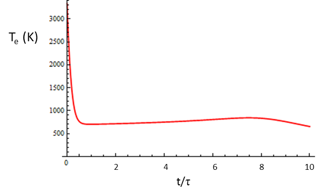
Figure 2: Time evolution of the electron temperature $T(t)$ for a hot, dense, population-inverted electron gas in graphene induced by an intense laser pulse at $t<0$. The initial temperature of this system, $T\left(0\right)=3336.4$ K, follows a sharp drop within a short time period $t<\tau/2$ mainly due to intra-band transitions, then reaches a plateau for a relatively longer time period $\tau/2<t<10\tau$ before further lowering down to the equilibrium temperature. Here $\tau=4\pi^{2}\hbar^{3}v^{2}/\left(a_{0}^{2}g^{2}\delta\mu\left(0\right)\right)\simeq 10.21$ ps.

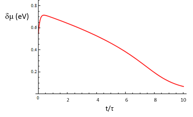
Figure 3: Time evolution of the population inversion $\delta\mu(t)$ for a hot, dense, population-inverted electron gas in graphene at the charge neutrality point where $\delta\mu(t)=\mu_{+}(t)=-\mu_{-}(t)$. The initial population inversion of this system, $\delta\mu\left(0\right)=0.549761$eV, follows a small jump within the short time period $t<\tau/2$ due to the establishment of the sharp Fermi-distribution edge that is associated with cooling, then decreases gradually as particle-hole recombination processes through inter-band transitions become dominate for the longer time period$\tau/2<t<10\tau$. Here $\tau\simeq 10.21$ ps.

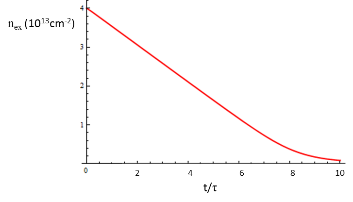
Figure 4: Time evolution of the carrier density $n_{\mathrm{ex}}(t)$ for a hot, dense, population-inverted electron gas in graphene. The photo-excited carrier density takes an initial value at $n_{\text{ex}}(t=0)=4\times 10^{13}$cm^-2, then drops gradually as a result of the inter-band carrier scattering processes through coupling to optical phonons. Here $\tau\simeq 10.21$ ps.

Three distinct time regimes during the relaxation of a initially hot dense state, with $k_{B}T(0)>\hbar\omega_{o}>k_{B}T_{L}$, are indicated from the numerical result: At short time scale, $t/\tau<1/2$, the electron temperature drops rapidly, while $\delta\mu$ rises due to the establishment of the sharp Fermi-distribution edge that is associated with cooling. While $n_{\text{ex}}$, decreasing slowly and linearly, is not sensitive to the rapid temperature drop and changes similar to the population inversion. The fast initial cooling is mainly due to carrier intra-band transitions by emitting optical phonons. This regime, dominated by carrier cooling process, characterizes the energy relaxation of the system. Next we identify an intermediate regime, $1/2<t/\tau<10$. In this regime we observe a plateau for the evolution of the electron temperature, while $\delta\mu\left(t\right)$ and $n_{\text{ex}}\left(t\right)$ decrease gradually. In this regime, the carrier cooling driven by intra-band transitions is less efficient while a relaxation dominated by inter-band transitions becomes dominant. This is the regime where the population inversion is being destroyed. Particle-hole recombination processes, characterize the population imbalance relaxation. Finally, for longer times, $t/\tau>10-20$, the relaxation of population inverted configurations is essentially completed and inter-band transitions from the upper to the lower branch becomes less significant. What is left is a slow cooling by the inefficient intra-band transition as $k_{B}T(t)\ll\hbar\omega_{o}$. In this regime, the coupling to acoustic phonons, ignored in our treatment, should come into play and eventually become the most dominant relaxation process for the terminal relaxation towards equilibrium.

IV Conclusions

In conclusion, we investigated post-transient state relaxation of hot, dense, population inverted electrons in graphene that emerged as the result of an intense laser pulse, as shown in Ref.Li2012 . Using a combination of hydrodynamic arguments and a kinetic theory we determined the cooling rate and charge-imbalance relaxation rate. The latter are determined from an analysis of the Boltzmann-equation where we included the scattering between electrons and optical phonons. We demonstrated that the relaxation of the electron temperature, driven by intra-band scattering processes, is much more rapid than the relaxation of the population inversion, which is determined by inter-band scattering processes. Thus, the relaxation of the population inversion is significantly slower that the timescales responsible for the energy transfers between the hot electron gas and the lattice. This insight may be of relevance for the application of graphene as an optical gain medium.

V
Acknowledgment

We thank Myron Hupalo and Michael Tringides for discussions. J.Z. acknowledges support by the Jeffress Memorial Trust, Grant No. J-1033. J.S. thanks the DFG Center for Functional Nanostructures. Work at Ames Laboratory was partially supported by the U.S. Department of Energy, Office of Basic Energy Science, Division of Materials Sciences and Engineering (Ames Laboratory is operated for the U.S. Department of Energy by Iowa State University under Contract No. DE-AC02-07CH11358).

References

(1) T. Li, L. Luo, M. Hupalo, J. Zhang, M. C. Tringides, J.
Schmalian, and J. Wang, Phys. Rev. Lett. 108, 167401 (2012).
(2) L. Fritz, J. Schmalian, M. Müller and S. Sachdev,
Physical Review B 78, 085416 (2008).
(3) M. Müller, J.Schmalian and L. Fritz, Phys. Rev. Lett.
103, 025301 (2009).
(4) M. S. Foster and I. L. Aleiner, Phys. Rev. B 79, 085415 (2009).
(6) R. Bistritzer and A. H. MacDonald, Phys. Rev. Lett.
102, 206410 (2009).
(7) W.-K. Tse and S. Das Sarma, Phys. Rev. B 79,
235406 (2009).
(8) S. Das Sarma, J. K. Jain, and R. Jalabert, Phys. Rev.
B 41, 3561 (1990); T. Kawamura, S. Das Sarma, R. Jalabert, and J.
K. Jain, Phys. Rev. B 42, 5407 (1990).
(9) D. E. Sheehy and J. Schmalian, Phys. Rev. Lett .
99 226803 (2007).
(10) S. Butscher, F. Milde, M. Hirtschulz, E. Malic, and A.
Knorr, Applied Physics Letters 91, 203103 (2007).