Possible Emission of Cosmic $X$– and $\gamma$–rays
by Unstable Particles at Late Times

Abstract

We find that charged unstable particles as well as neutral unstable particles with non–zero magnetic moment which live sufficiently long may emit electromagnetic radiation. This new mechanism is connected with the properties of unstable particles at the post exponential time region. Analyzing the transition times region between exponential and non-exponential form of the survival amplitude it is found that the instantaneous energy of the unstable particle can take very large values, much larger than the energy of this state for times from the exponential time region. Based on the results obtained for the model considered, it is shown that this purely quantum mechanical effect may be responsible for causing unstable particles to emit electromagnetic–, $X$– or $\gamma$–rays at some time intervals from the transition time regions.

PACS: 98.70.-f, 98.70.Sa, 98.80.-k, 11.10.St
Key words: Unstable states, post–exponential decay, late time deviations, cosmic $\gamma$–rays

1 Introduction

Not all astrophysical mechanisms of the emission of electromagnetic radiation including $X$– and $\gamma$– rays coming from the space are clear. Typical physical processes in which cosmic microwave and other electromagnetic radiation, $X$–, or $\gamma$-rays are generated have purely electromagnetic nature (an acceleration of charged particles, inverse Compton scattering, etc.), or have the nature of nuclear and particle physics reactions (particle–antiparticle annihilation, nuclear fusion and fission, nuclear or particle decay). The knowledge of these processes is not sufficient for explaining all mechanisms driving the emission from some galactic and extragalactic $X$– or $\gamma$–rays sources, e.g. the mechanism that generates $\gamma$–ray emission of the so-called ”Fermi bubbles” remains controversial, the mechanisms which drive the high energy emission from blazars is still poorly understood, etc. (see eg. [1, 2, 3, 4]). Similar problems can be encountered when trying to explain the mechanism of radiation of some cosmic radio sources: Origin of some radio bursts and many of other sources is still unknown (see, eg. [5, 6]) and the radiation mechanism is unclear and, at the best, insufficiently clear. Astrophysical processes are the source of not only electromagnetic, $X$- or $\gamma$-rays but also a huge number of elementary particles including unstable particles of very high energies (see eg. [4]). The numbers of created unstable particles during these processes are so large that many of them can survive up to times $t$ at which the survival probability depending on $t$ transforms from the exponential form into the inverse power–like form. It appears that at this time region a new quantum effect is observed: A very rapid fluctuations of the instantaneous energy of unstable particles take place. These fluctuations of he instantaneous energy should manifest themselves as fluctuations of the velocity of the particle. We show that this effect may cause unstable particles to emit electromagnetic radiation of a very wide spectrum: from radio– up to ultra–high frequencies $\nu$ including $X$–rays and $\gamma$–rays.

To make the paper easily understandable we start in Sec. 2 with a brief introduction into the problem of the late time behavior of unstable states. In Sec. 3 late time properties of the a energy of unstable states are analyzed. In Sec. 4 observable effects are discussed: The emission of electromagnetic radiation by unstable particles created in astrophysical processes. Final Section provides a short summary and suggestions where to look for signs of the effect described in Sec. 4.

2 Late time properties of unstable states

Searching for the properties of unstable states one usually analyzes their decay law, i. e. their survival probability: If $|\phi\rangle$ is an initial unstable state then the survival probability, ${\cal P}(t)$, equals ${\cal P}(t)=|a(t)|^{2}$, where $a(t)$ is the survival amplitude, $a(t)=\langle\phi|\phi;t\rangle$, and $|\phi;t\rangle=e^{\textstyle{-itH}}\,|\phi\rangle$, $H$ is the total Hamiltonian of the system under considerations, $|\phi\rangle,|\phi;t\rangle\in{\cal H}$ and ${\cal H}$ is the Hilbert space of states of the considered system. The spectrum, $\sigma(H)$, of $H$ is assumed to be bounded from below, $\sigma(H)=[E_{min},\infty)$ and $E_{min}>-\infty$. Studying the late time properties of unstable states it is convenient to use the integral representation of $a(t)$ as the Fourier transform of the energy distribution function, $\omega(E)$,

$$a(t)=\int\,\omega(E)\,e^{\textstyle{-itE}}\,dE,$$ (1)

with $\omega(E)\geq 0$ and $\omega(E)=0$ for $E<E_{min}$ [7, 8, 9, 10, 11, 12, 13, 14, 15, 16]. In the case of quasi–stationary (metastable) states it is useful to express $a(t)$ in the following form [14, 15], $a(t)=a_{exp}(t)+a_{lt}(t)$, where $a_{exp}(t)$ is the exponential part of $a(t)$, that is $a_{exp}(t)=N\,\exp\,[{-it(E_{\phi}^{0}-\frac{i}{2}\,{\it\Gamma}_{\phi}^{0})}]$, ($E_{\phi}^{0}$ is the energy of the system in the state $|\phi\rangle$ measured at the canonical decay times, i.e. when ${\cal P}_{\phi}(t)$ has the exponential form, ${\it\Gamma}_{\phi}^{0}$ is the decay width, $N$ is the normalization constant), and $a_{lt}(t)$ is the late time non–exponential part of $a(t)$.

From the literature it is known that the characteristic feature of survival probabilities ${\cal P}(t)$ is the presence of sharp and frequent fluctuations at the transition times region, when contributions from $|a_{exp}(t)|^{\,2}$ and $|a_{lt}(t)|^{\,2}$ into ${\cal P}(t)$ are comparable (see, eg. [8, 10, 11, 12, 13]), and that the amplitude $a_{lt}(t)$ and thus the probability ${\cal P}(t)$ exhibits inverse power–law behavior at the late time region for times $t$ much later than the crossover time $T$. (This effect was confirmed experimentally not long ago [17]). The crossover time $T$ can be found by solving the following equation, $|a_{exp}(t)|^{\,2}=|a_{lt}(t)|^{\,2}$. In general $T\gg\tau_{\phi}$, where $\tau_{\phi}=1/{\it\Gamma}^{0}_{\phi}$ is the live–time of $\phi$. Formulae for $T$ depend on the model considered (i.e. on $\omega(E)$) in general (see, eg. [9, 10, 11, 14, 15, 16]). The standard form of the decay curve, that is the form of the probability ${\cal P}(t)$ as a function of time $t$ is presented in Fig. (1). In this Figure the calculations were performed using the Breit–Wigner energy distribution function, $\omega({E})\equiv\omega_{BW}(E)$, where

$$\omega_{BW}(E)\stackrel{{\scriptstyle\rm def}}{{=}}\frac{N}{2\pi}{\it\Theta}(E-E_{min})\frac{{\it\Gamma}_{\phi}^{0}}{(E-E_{\phi}^{0})^{2}+(\frac{{\it\Gamma}_{\phi}^{0}}{2})^{2}},$$ (2)

and $\it\Theta({E})$ is the unit step function. In Fig. (1) calculations were performed for $({E_{\phi}^{0}}-E_{min})/{{\it\Gamma}_{\phi}^{0}}=20$.

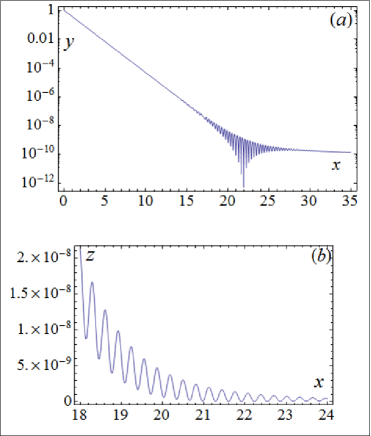
Figure 1: Axes: $x=t/\tau_{\phi},y={\cal P}(t)$ — the logarithmic scale, $z={\cal P}(t)$. (a) The general, typical form of the decay curve ${\cal P}(t)$. (b) An enlarged part of (a) showing a typical behavior of the survival probability ${\cal P}(t)$ at the transition times region when $t\sim T$.

Deviations form the exponential decay law visible in Fig. (1) are caused by the regeneration process [8, 18, 19]. A certain fixed proportion between rates of decay and regeneration processes does not change at canonical decay times, so there is a kind of a balance between these processes at this time region. This balance is broken at transition times and later. Oscillations of the decay law seen in the transition times region are a reflection of this fact. Time intervals around local maxima of the decay curve presented in the panel (b) of Fig. (1) are places where the regeneration process begins to dominate temporarily and the decay process slows down. On the other hand, times close to the local minima fix places where the regeneration rate is minimal and the decay process accelerates.

Note that the survival amplitude $a(t)$ obtained within quantum mechanics share with the amplitude $a(t)$ obtained as a result of investigations on relativistic quantum field theory models, the property (1) of being the Fourier transform of a positive definite function $\omega(E)$ with a limited from below support (see, eg. [9, 20, 21, 22, 23]). This means that effects connected with the long time behavior at $t\sim T$ and $t\gg T$ of the survival probability ${\cal P}(t)$ should take place in the both cases: When they are considered at the level of quantum mechanical processes as well as at the level of the processes that require quantum field theory to describe them.

3 Energy of unstable states at late times

It is commonly known that the information about the decay rate, $\it\Gamma_{\phi}$, of the unstable state $|\phi\rangle$ under considerations can be extracted from the survival amplitude $a(t)$. In general not only $\it\Gamma_{\phi}$ but also the instantaneous energy ${\cal E}_{\phi}(t)$ of an unstable state $|\phi\rangle$ can be calculated using $a(t)$ [14, 15]. In the considered case, ${\cal E}_{\phi}(t)$ can be found using the effective Hamiltonian, $h_{\phi}(t)$, governing the time evolution in an one–dimensional subspace of states spanned by vector $|\phi\rangle$, [14, 15]:

$$h_{\phi}(t) = \frac{i}{a(t)}\,\frac{\partial a(t)}{\partial t}$$ (3)

$$\equiv \frac{\langle\phi|H|\phi;t\rangle}{\langle\phi|\phi;t\rangle}.$$ (4)

The instantaneous energy ${\cal E}_{\phi}(t)$ of the system in the state $|\phi\rangle$ is the real part of $h_{\phi}(t)$, ${\cal E}_{\phi}(t)=\Re\,(h_{\phi}(t))$. The imaginary part of $h_{\phi}(t)$ defines the instantaneous decay rate $\it\Gamma_{\phi}(t)$, ${\it\Gamma}_{\phi}\equiv{\it\Gamma}_{\phi}(t)=-2\,\Im\,(h_{\phi}(t))$, [24, 14, 15].

There is ${\cal E}_{\phi}(t)=E_{\phi}^{0}$ and ${\it\Gamma}_{\phi}(t)={\it\Gamma}_{\phi}^{0}$ at the canonical decay times (see, eg., [24]) and at asymptotically late times (see [15, 14, 25]),

$${\cal E}_{\phi}(t) \simeq E_{min}+\frac{c_{2}}{t^{2}}\,+\,\frac{c_{4}}{t^{4}}\ldots,\;\;\;({\rm for}\;\;t\gg T),$$ (5)

$$\it\Gamma_{\phi}(t) \simeq \frac{c_{1}}{t}+\frac{c_{3}}{t^{3}}+\ldots\;\;\;({\rm for}\;\;t\gg T),$$ (6)

where $c_{i}=c_{i}^{\ast},\;i=1,2,\ldots$, ($c_{1}>0$ and the sign of $c_{i}$ for $i\geq 2$ depends on the model considered), so $\lim_{t\rightarrow\infty}\,{\cal E}_{\phi}(t)=E_{min}$ and $\lim_{t\rightarrow\infty}\,{\it\Gamma}_{\phi}(t)=0$ [15, 14, 25]. Results (5) and (6) are rigorous. The basic physical factor forcing the amplitude $a(t)$ to exhibit inverse power law behavior at $t\gg T$ is the boundedness from below of $\sigma(H)$. This means that if this condition is satisfied and $\int_{-\infty}^{+\infty}\omega(E)\,dE\,<\,\infty$, then all properties of $a(t)$, including the form of the time–dependence at $t\gg T$, are the mathematical consequence of them both. The same applies by (3) to the properties of $h_{\phi}(t)$ and concerns the asymptotic form of $h_{\phi}(t)$ and thus of ${\cal E}_{\phi}(t)$ and $\it\Gamma_{\phi}(t)$ at $t\gg T$.

The sharp and frequent of fluctuations of ${\cal P}(t)$ at the transition times region (see Fig. (1)) are a consequence of a similar behavior of real and imaginary parts of the amplitude $a(t)$ at this time region. Therefore the derivatives of $a(t)$ may reach extremely large negative and positive values for some times from the transition time region and the modulus of these derivatives is much larger than the modulus of $a(t)$, which is very small for these times. This means that at this time region the real part of $h_{\phi}(t)$ which is expressed by the relation (3), i. e. by a large derivative of $a(t)$ divided by a very small $a(t)$, can reach values much larger than the energy ${E}_{\phi}^{0}$ of the unstable state measured at the canonical decay times. Using relations (1), (3) and assuming the form of $\omega(E)$ and performing all necessary calculations numerically one can see how this mechanism work. A typical behavior of the instantaneous energy ${\cal E}_{\phi}(t)$ at the transition time region is presented in Figs (3) and (3). In these figures the calculations were performed for the Breit–Wigner energy distribution function (2).

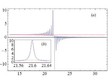
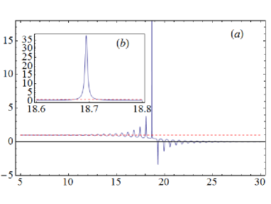
Figure 2: Axes: $y=({\cal E}_{\phi}(t)-E_{min})/(E_{\phi}^{0}-E_{min})$, $x=t/\tau_{\phi}$. The dashed line denotes the straight line $y=1$. (a) The instantaneous energy ${\cal E}_{\phi}(t)$ in the transitions time region: The case $({E_{\phi}^{0}}-E_{min})/{{\it\Gamma}_{\phi}^{0}}=20$. (b) Enlarged part of (a): The highest maximum of $({\cal E}_{\phi}(t)-E_{min})/(E_{\phi}^{0}-E_{min})$ in the transition times region.

Figure 3: The same as in Fig (1) for $({E_{\phi}^{0}}-E_{min})/{{\it\Gamma}_{\phi}^{0}}=10$.

From (4) it follows that the effective Hamiltonian $h_{\phi}(t)$ is the so-called weak value of $H$ [26, 27, 28, 29]. Considering $h_{\phi}(t)$ as a weak value the behavior of ${\cal E}_{\phi}(t)$ at transition times region and extremely large values reached by ${\cal E}_{\phi}(t)$ at some times there that can be seen in Figs (3) and (3) are not extraordinary effects. Properties of this kind are typical for many weak values of physical quantities [26, 27, 28, 29]. What is more experiments have verified aspects of the theory of weak values (see, eg. [28, 29, 30, 31, 32, 33]).

It seems that one should observe a picture presented in Figs (3), (3), or similar one, e.g. after performing a suitable modification of the experiment described in [17]. This modification should allow one to register not only the presence of the photons emitted by excited molecules but also energies of these photons (i.e. frequencies of the registered radiation). Analogous modifications of possible experiments based on the effects analyzed in [34] and proposed there seems to make such the observation possible.

More detailed numerical analysis of ${\cal E}_{\phi}(t)$ and ${\cal P}(t)$ within the model considered shows that local maxima of $({\cal E}_{\phi}(t)-E_{min})/(E_{\phi}^{0}-E_{min})$ correspond with the local minima of the survival probability ${\cal P}(t)$ (see Fig. (4)). It is just as one would expect: The higher the energy ${\cal E}_{\phi}(t)$, i. e., the greater the difference $({\cal E}_{\phi}(t)-E_{min})$ the higher the probability of a decay (i. e., the survival probability less). One meets an analogous effect in the case of the local minima of $({\cal E}_{\phi}(t)-E_{min})/(E_{\phi}^{0}-E_{min})$: They correspond with the local maxima of the survival probability. There is a simple and obvious interpretation of this effect: The difference $({\cal E}_{\phi}(t)-E_{min})$ smaller the decay process slower and the regeneration process faster.

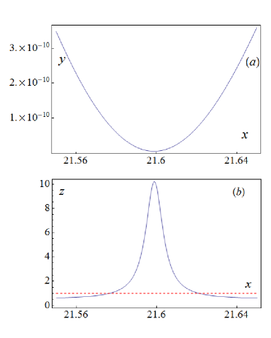
Figure 4: Axes: $x=t/\tau_{\phi},y={\cal P}(t)$, $z=({\cal E}_{\phi}(t)-E_{min})/(E_{\phi}^{0}-E_{min})$. The case $({E_{\phi}^{0}}-E_{min})/{{\it\Gamma}_{\phi}^{0}}=20$. (a) The local minimum of ${\cal P}(t)$ corresponding with the highest local maximum of the ratio $({\cal E}_{\phi}(t)-E_{min})/(E_{\phi}^{0}-E_{min})$. (b) The highest local maximum of $({\cal E}_{\phi}(t)-E_{min})/(E_{\phi}^{0}-E_{min})$.

From the results presented in Figs (3) and (3) one can see that the ratio, $({\cal E}_{\phi}(t)-E_{min})/(E_{\phi}^{0}-E_{min})$, takes negative values for some times at transition times region. This does not mean that the instantaneous energy ${\cal E}_{\phi}(t)$ of the unstable particle takes negative negative values at these times $t$. The negative values of $({\cal E}_{\phi}(t)-E_{min})/(E_{\phi}^{0}-E_{min})$ mean that ${\cal E}_{\phi}(t)>0$ becomes smaller than $E_{min}$ at these $t$. The most negative values of this ratio occur in its local minima, which correspond to local maxima of the survival probability ${\cal P}(t)$ as it was mentioned above. This means that at these times the rate of the decay process greatly slows down and even nearly stops but the rate of the regeneration process becomes extremely fast.

4 Observable effects

Note that from the point of view of a frame of reference in which the time evolution of the unstable system was calculated the Rothe experiment as well as the picture presented in Figs (3), (3) refer to the rest coordinate system of the unstable system considered. Astrophysical sources of unstable particles emit them with relativistic or ultra–relativistic velocities in relation to an external observer so many of these particles move in space with ultra high energies. The question is what effects can be observed by an external observer when the unstable particle, say $\phi$, which survived up to the transition times region, $t\sim T$, or longer is moving with a relativistic velocity in relation to this observer. The distance $d$ from the source reached by this particle is of order $d\sim d_{T}$, where $d_{T}=v^{\phi}\cdot T^{\prime},\,T^{\prime}=\gamma_{L}\,T$ and $\gamma_{L}\equiv\gamma_{L}(v^{\phi})=(\sqrt{1-\beta^{2}})^{-1}$, $\beta=v^{\phi}/c$, $v^{\phi}$ is the velocity of the particle $\phi$. (For simplicity we assume that there is a frame of reference common for the source and observer both and that they do not move with respect to this frame of reference). The relation (4) explains why effects of type (5), (6) and those one can see in Figs (3), (3) are possible. In the case of moving particles created in astrophysical processes one should consider the effect shown in Figs (3), (3) together with the fact that the particle gains extremely huge kinetic energy, $W^{\phi}$, which have to be conserved. There is $W^{\phi}=m^{0}_{\phi}\ c^{2}\ \gamma_{L}$, where $m_{\phi}^{0}$ is the rest mass of the particle $\phi$. We have $m_{\phi}^{0}\ c^{2}\equiv E_{\phi}^{0}$ at canonical decay times and thus $W^{\phi}\equiv E_{\phi}^{0}\ \gamma_{L}$ at these times. At this time region $E_{\phi}^{0}={\cal E}_{\phi}(t)$ but at times $t\gg\tau_{\phi},\;t\sim T$ we have ${\cal E}_{\phi}(t)\neq E_{\phi}^{0}$. A general relation between instantaneous energies of the unstable particle in the rest system and in the system connected with the moving particle can be found using a relation between the survival amplitude, $a^{v\neq 0}(t)$, of a moving unstable particle and the survival amplitude, $a^{v=0}(t)$, of the particle in the rest coordinate system of the observer $\cal O$. In such a case assuming that the rest system of the particle moves with a velocity $v^{\phi}$ relative to $\cal O$ one can find within the relativistic quantum theory that (see eg. [35])

$$a^{v\neq 0}(t)=a^{v=0}(\frac{t}{\gamma_{L}}).$$ (7)

The relation (7) means that survival probabilities ${\cal P}^{v\neq 0}(t)$ and ${\cal P}^{v=0}(t/\gamma_{L})$ corresponding with the survival amplitudes $a^{v\neq 0}(t)$, $a^{v=0}(t/\gamma_{L})$ respectively are equal. This property and thus the relation (7) was tested by numerous experiments. Now using (3) and (7) it is easy to find that

$$h_{\phi}^{v\neq 0}(t)=\frac{1}{\gamma_{L}}\,h_{\phi}^{v=0}(t/\gamma_{L}),$$ (8)

where $h_{\phi}^{v\neq 0}(t)$ is obtained by inserting into (3) the survival amplitude $a^{v\neq 0}(t)$, and so on. From this last relation is follows that the instantaneous energy ${\cal E}^{v=0}_{\phi}(t/\gamma_{L})=\Re\,(h_{\phi}^{v=0}(t/\gamma_{L}))$ of the moving particle $\phi$ measured by the observer ${\cal O}$ equals ${\cal E}^{v=0}_{\phi}(t/\gamma_{L})=\gamma_{L}\,{\cal E}^{v\neq 0}_{\phi}(t)$. Taking into account that ${\cal E}^{v\neq 0}_{\phi}(t)=\Re\,(h_{\phi}^{v\neq 0}(t))$ is the instantaneous energy measured in the rest system of the particle one can identify it with the instantaneous energy ${\cal E}_{\phi}(t)$ analyzed in the previous Section. So in the general case the kinetic energy of the moving particle $\phi$ having the energy ${\cal E}_{\phi}^{k}$ in its rest system measured by the observer ${\cal O}$ equals $W_{k}^{\phi}=\gamma_{L}^{k}\,{\cal E}_{\phi}^{k}$ and here $\gamma_{L}^{k}=\gamma_{L}(v^{\phi}_{k})$. Similarly there is $W_{l}^{\phi}=\gamma_{L}^{l}\,{\cal E}_{\phi}^{l}$ for the other particle moving with the velocity $v^{\phi}_{l}\neq v^{\phi}_{k}$ and having the energy ${\cal E}_{\phi}^{l}$. Now if to assume that we observe the particle $\phi$ at different instants $t_{k}\neq t_{l}$ of time $t$ then we can use the following identification: ${\cal E}_{\phi}^{k(l)}={\cal E}_{\phi}(t_{k(l)})$. Of course the kinetic energies $W^{\phi},W^{\phi}_{k},W^{\phi}_{l}$ of $\phi$ have to be the same at the canonical decay times region and at the transition times $t_{k},\,t_{l}\,\sim\,T$: $W^{\phi}\equiv W^{\phi}_{k}\equiv W^{\phi}_{l}$, that is there should be

$$W^{\phi}\equiv\gamma_{L}^{k}\,{\cal E}_{\phi}^{k}\,=\,const.$$ (9)

From relation (9) one can infer that this is possible only when the changes of ${\cal E}_{\phi}(t_{k})$ at times $t_{k}\sim T$ are balanced with suitable changes of $\gamma_{L}^{k}$ (i.e. of the velocity $v^{\phi}_{k}$ of the considered particle). So, in the case of moving unstable particles, an external observer should detect rapid fluctuations (changes) of their velocities at distances $d\sim d_{T}$ from their source. These fluctuations of the velocities mean for the observer that the particles are moving with a nonzero acceleration in this space region, $\dot{v^{\phi}}\neq 0$. So we can expect that this observer will register electromagnetic radiation emitted by charged unstable particles, which survived up to times $t\sim T$, i.e. which reached distances $d\sim d_{T}$ from the source (see Fig (5)).

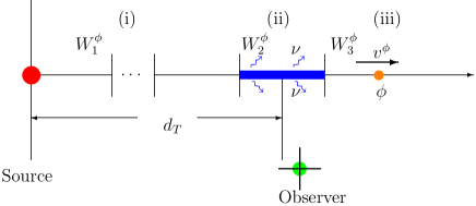
Figure 5: Time regions: (i) Canonical decay, (ii) Transition, (iii) Asymptotically late. $W_{i}^{\phi}=\gamma_{L}^{i}\,{\cal E}_{\phi}^{i},\;(i=1,2,3)$ and $W_{i}^{\phi}$ is the energy of moving relativistic particle $\phi$ measured by the observer, ${\cal E}_{\phi}^{i}={\cal E}_{\phi}(t_{i})$, $t_{1}\ll t_{2}\ll t_{3}$, $t_{1}\sim\tau_{\phi}$, $t_{2}\sim T$, $t_{3}\gg T$ and $W^{\phi}_{1}=E_{\phi}^{0}\gamma_{L}^{1}$, $\nu$ is the frequency of the emitted electromagnetic rays.

This follows from the Larmor formula and its relativistic generalization, which state that the total radiation power, $P$, from the considered charged particle is proportional to $(\dot{v^{\phi}})^{2}$ (see eg. [36]):

$$P=\frac{1}{6\pi\epsilon_{0}}\,\frac{q^{2}\,({\dot{v^{\phi}}})^{2}}{c^{2}}\,\gamma_{L}^{6},$$ (10)

(where $q$ is the electric charge, ${\epsilon}_{0}$ – permittivity for free space), and $\dot{v^{\phi}}\neq 0$ implies that there must be $P\neq 0$. The same conclusion also concerns neutral unstable particles with non–zero magnetic moment [36, 37]. One should expect that the spectrum of this radiation will be very wide: From high radio frequencies, through $X$–rays up to high energy $\gamma$–rays depending on the scale of the fluctuations of the instantaneous energy ${\cal E}_{\phi}(t)$ in this space region.

Within the model defined by $\omega_{BW}(E)$ the cross–over time $T$ can be found using the following approximate relation valid for ${E_{\phi}^{0}}/{\it\Gamma_{\phi}^{0}}\gg 1$, [14]:

$${\it\Gamma}_{\phi}^{0}\,T\equiv\frac{T}{\tau_{\phi}}\;\sim\;2\,\ln\,\Big{[}2\pi\Big{(}\frac{E_{\phi}^{0}-E_{min}}{\it\Gamma_{\phi}^{0}}\Big{)}^{2}\Big{]},$$ (11)

whereas for the model considered in [16, 9] one has ${T}/{\tau_{\phi}}\;\sim\;5\,\ln\big{[}({E_{\phi}^{0}}-E_{min})/{{\it\Gamma}_{\phi}^{0}}\big{]}$ (see (11) in [16]). Considering a meson $\mu^{\pm}$ as an example and taking $E_{\phi}^{0}-E_{min}=m_{\mu^{\pm}}-(m_{e}+m_{\bar{\nu}_{e}}+m_{\nu_{\mu}})\simeq 105$ [MeV], then using (11) one finds $T=T_{\mu}\sim 165.3\,\tau_{\mu}$. (The formula (11) from [16] gives $T_{\mu}\sim 202\,\tau_{\mu}$). The distance $d_{T_{\mu}}$ from the source reached by muon, which survived up to the time $T_{\mu}\simeq 165.3\,\tau_{\mu}$ depends on its kinetic energy $W^{\mu}$ and equals: from $d_{T_{\mu}}\simeq 10^{6}$ [m] if $W^{\mu}=10^{9}$ [eV], up to $d_{T_{\mu}}\simeq 0.033$ [pc] if $W^{\mu}=10^{18}$ [eV]. Similarly, there is for $\pi$–mesons $E_{\phi}^{0}-E_{min}=m_{\pi^{\pm}}-(m_{\mu^{\pm}}+m_{\nu_{\mu}})\simeq 33.83$ [MeV], which leads by (11) to the results: $T_{\pi^{\pm}}\simeq 143\;\tau_{\pi^{\pm}}$ and $d_{T_{\pi^{\pm}}}7.9\simeq\times 10^{3}$ [m] if $W^{\pi}=10^{9}$ [eV] and $d_{T_{\pi^{\pm}}}\simeq 8\times 10^{12}$ [m] $\simeq 53.45$ [au] if $W^{\pi}=10^{18}$ [eV]. For the neutron $E_{\phi}^{0}-E_{min}=m_{n}-(m_{p}+m_{e}+m_{\nu_{e}})\simeq 0.78$ [MeV] and using (11) one finds: $T_{n}\simeq 225\;\tau_{n}$ and $d_{T_{n}}\simeq 130.6$ [au] if $W^{n}=10^{9}$ [eV] and $d_{T_{n}}\simeq 2.05$ [Mpc] if $W^{n}=10^{18}$ [eV].

Let us now analyze Fig (3) in more details. Coordinates of the highest maximum in Fig (3) are equal: ($x_{mx},y_{mx})=(21.60,10.27)$. Coordinates of points of the intersection of this maximum with the straight line $y=1$ are equal: $(x_{1},y_{1})=(21.58,1.0)$ and $(x_{2},y_{2})=(21.62,1.0)$. From these coordinates one can extract the change $\Delta v^{\phi}=v^{\phi}_{M}-v^{\phi}_{1}$ of the velocity $v^{\phi}$ of the considered particle and the time interval $\Delta t=t_{M}-t_{1}$ at which this change occurred (Here $t_{M}=t_{mx}$ and $v^{\phi}_{1}=v^{\phi}(t_{1})$). Indeed, using (9) one finds

$$\gamma_{L}^{1}=\frac{{\cal E}_{\phi}^{M}}{{\cal E}_{\phi}^{1}}\;\gamma_{L}^{M}.$$ (12)

There are ${\cal E}_{\phi}^{M}={\cal E}_{\phi}(t_{M})$ and ${\cal E}_{\phi}^{1}={\cal E}_{\phi}(t_{1})\equiv E^{0}_{\phi}$ in the considered case. This means that we can replace $\gamma_{L}^{1}$ by $\gamma_{L}$ measured at the canonical decay times and then taking the value of the ratio ${\cal E}_{\phi}^{M}/E_{\phi}^{0}$ from Fig (3) we can use (12) to calculate $\gamma_{L}^{M}$. Figs (3), (3) show how the ratio $({\cal E}_{\phi}(t)-E_{min})/(E_{\phi}^{0}-E_{min})\stackrel{{\scriptstyle\rm def}}{{=}}\kappa(t)$ varies in time and this $\kappa(t)$ can be easy extracted form these Figures, eg., for $t=t_{M}$ and for $t=t_{1}\neq t_{M}$. If one wants to use the relation (12) in order to calculate $\gamma_{L}^{M}$, one needs the ratio ${\cal E}_{\phi}(t)/E_{\phi}^{0}$ instead of $\kappa(t)$. Using $\kappa(t)$ it is easy to express ${\cal E}_{\phi}(t)/E_{\phi}^{0}$ in terms of known parameters of unstable particles considered. We have

$$\frac{{\cal E}_{\phi}(t)}{E_{\phi}^{0}}=\kappa(t)\,-\,\big{(}\kappa(t)\,-\,1\big{)}\,\frac{E_{min}}{E_{\phi}^{0}}.$$ (13)

In the considered case $\kappa(t_{M})\equiv y_{mx}=10.27$ which, eg., for the muon gives ${\cal E}_{\mu}^{M}/E_{\phi}^{0}\simeq 10.21$. Hence using (12) within the considered model one finds that for the muon there is $\gamma_{L}^{1}\simeq 10.21\,\gamma_{L}^{M}$. Next having $\gamma_{L}^{1}\equiv\gamma_{L}$ and $\gamma_{L}^{M}$ it is easy to find $\Delta v^{\phi}=v^{\phi}_{M}-v^{\phi}_{1}$. Now using (10) one can estimate the energy $P$ of the electromagnetic radiation emitted in unit of time by an unstable charged relativistic particle $\phi$ during the time interval $\Delta t$. In other words, one can find $\Delta v^{\phi}/\Delta t$ and thus $P\propto(\Delta v^{\phi}/\Delta t)^{2}$. This procedure, formulae (9), (12) and parameters describing the highest maximum in Fig. (3) lead to the following (simplified, very conservative) estimations of the energies of the electromagnetic radiation emitted by ultra relativistic muon at the transition times region (in a distance $d\sim d_{T}$ from the source): $P\sim 4.6$ [eV/s]. Analogously coordinates of the highest maximum in Fig (3) are equal: ($x_{mx},y_{mx})=(18.69,37.68)$ and coordinates of points of the intersection of this maximum with the line $y=1$ are: $(x_{1},y_{1})=(18.67,1.0)$ and $(x_{2},y_{2})=(18.72,1.0)$. This leads to the following estimation: $P\sim 0.84$ [keV/s]. Similar estimations of $P$ can be found for neutral ultra–relativistic unstable particles with non–zero magnetic moment.

The question is where the above described effect may be observed. Astrophysical and cosmological processes in which extremely huge numbers of unstable particles are created seem to be a possibility for the above discussed effect to become manifest. The fact is that the probability ${\cal P}_{\phi}(t)=|a(t)|^{2}$ that an unstable particle $\phi$ survives up to time $t\sim T$ is extremely small. Let ${\cal P}_{\phi}(t)$ be ${{\cal P}_{\phi}(t)\,\vline}_{\;t\sim T}\;\sim\;10^{-k}$, where $k\gg 1$, then there is a chance to observe some of particles $\phi$ survived at $t\sim T$ only if there is a source creating these particles in ${\cal N}_{\phi}$ number such that ${{\cal P}_{\phi}(t)\,\vline}_{\;t\sim T}\;{\cal N}_{\phi}\;\gg\;1$. So if a source exists that creates a flux containing ${\cal N}_{\phi}\;\sim\;10^{\,l}$, unstable particles and $l\gg k$ then the probability theory states that the number $N_{surv}$ of unstable particles $N_{surv}={{\cal P}_{\phi}(t)\,\vline}_{\;t\sim T}\;{\cal N}_{\phi}\;\sim\;10^{l-k}\;\gg\;1$, has to survive up to time $t\sim T$. Sources creating such numbers of unstable particles are known from cosmology and astrophysics: as example of such a source can be considered processes taking place in galactic nuclei (galactic cores), inside stars, etc. According to estimations of the luminosity of some $\gamma$–rays sources the energy emitted by these sources can even reach a value of order $10^{52}$ [erg/s], [4, 38, 39, 40], and it is only a part of the total energy produced there. So, if one has a source emitting energy $10^{50}$ [erg/s] then, eg., an emission of ${\cal N}_{0}\simeq 6.25\times 10^{47}$ [1/s] particles of energy $10^{18}$ [eV] is energetically allowed. The same source can emit ${\cal N}_{0}\simeq 6.25\times{10}^{56}$ [1/s] particles of energy $10^{9}$ [eV] and so on. If one follows [16] and assumes that for laboratory systems a typical value of the ratio ${(E_{\phi}^{0}}-E_{min})/{{\it\Gamma}_{\phi}^{0}}$ is $({E_{\phi}^{0}}-E_{min})/{{\it\Gamma}_{\phi}^{0}}\,\geq\,O(10^{3}-10^{6})$ and then taking, eg. $({E_{\phi}^{0}}-E_{min})/{{\it\Gamma}_{\phi}^{0}}=10^{6}$ one obtains from (11) that ${\cal N}_{\phi}(T)\sim 2.53\times 10^{-26}\,{\cal N}_{0}$ and from the estimation of $T$ used in [16] (see (11), (12) in [16]) that ${\cal N}_{\phi}(T)\sim 10^{-30}\,{\cal N}_{0}$. This means that there are ${\cal N}_{\phi}(T)\sim 14\times 10^{21}$ particles per second of energy $W^{\phi}=10^{18}$ [eV] or ${\cal N}_{\phi}(T)\sim 14\times 10^{30}$ particles of energy $W^{\phi}=10^{9}$ [eV] in the case of the considered example and $T$ calculated using (11). On the other hand from $T$ obtained for the model considered in [16] one finds ${\cal N}_{\phi}(T)\sim 6.25\times 10^{17}$ and ${\cal N}_{\phi}(T)\sim 6.25\times 10^{26}$ respectively. These estimations show that astrophysical sources are able to create such numbers ${\cal N}_{0}$ of unstable particles that sufficiently large number ${\cal N}_{\phi}(T)\gg 1$ of them has to survive up to times $T$ when the effect described above should occur. So the numbers of unstable particles produced by some astrophysical sources are sufficiently large in order that a significant part of them had to survive up to the transition times and therefore to emit electromagnetic radiation. The expected spectrum of this radiation can be very wide: From radio frequencies up to $\gamma$–rays depending on energy distribution function $\omega(E)$ of the unstable particle emitting this radiation.

5 Final remarks

We have shown that charged unstable particles or neutral unstable particles with non–zero magnetic moment, which survived up to transition times or longer, should emit electromagnetic radiation. We have also shown that only astrophysical processes can generate sufficiently huge number of unstable particles in order that this emission could occur. From our analysis it seems to be clear that the effect described in this paper may have an astrophysical meaning and help explain the controversies, which still remain, concerning the mechanisms that generates the cosmic microwave, or $X$–, or $\gamma$–rays emission, e.g. it could help explain why some space areas (bubbles) without visible astronomical objects emit microwave radiation, $X$– or $\gamma$–rays. Indeed, let us consider active galactic nuclei as an example. They emit extremely huge numbers of stable and unstable particles including neutrons (see eg. [2]) along the axis of rotation of the galaxy. The unstable particles, which reached distances $d\sim d_{T}$ from the galactic plane, should emit electromagnetic radiation. So a distant observer should detect enhanced emission of this radiation coming from bubbles with the centra located on the axis of the galactic rotation at average distances $d_{T}$ from the galactic plane (see Fig. (5)). In the case of neutrons $d_{T_{n}}$ can be extremely large. Therefore a possible emission of the electromagnetic radiation generated by neutrons surviving sufficiently long seems to be relatively easy to observe and it should be possible to determine $d_{T_{n}}$. Now having realistic sufficiently accurate $\omega(E)$ for neutrons we are able to calculate $T_{n}$ and to find ${\cal E}_{n}(t)$ and its local maxima at transition times. Thus if the energies $W^{n}$, (i.e., $\gamma_{L}$), are known then in fact we know velocities $v^{n}$ and we can compute $d_{T_{n}}$ and distances where ${\cal E}_{n}(t)$ has maxima. All these distances fix the space areas where the mechanism discussed should manifest itself. This suggests how to test this mechanism: The computed $d_{T_{n}}$ can be compared with observational data and thus one can test if the mechanism described in our letter works in astrophysical processes.

Note that all possible effects discussed in this paper are the simple consequence of the fact that the instantaneous energy ${\cal E}_{\phi}(t)$ of unstable particles becomes large for suitably long times compared with $E_{\phi}^{0}$ and for some times even extremely large. This property of ${\cal E}_{\phi}(t)$ is a purely quantum effect resulting from the assumption that the energy spectrum is bounded from below and it was found by performing an analysis of the properties of the quantum mechanical survival probability $a(t)$.

Acknowledgments: This work was supported in part (KU) by the Polish NCN project 2013/09/B/ST2/03455.

References

- [1] J. Holder, Astropart. Phys. 39–40, 61 (2012).
- [2] L. A. Anchordoqui, H. Goldberg, T. J. Weiler, Phys. Rev. Lett., 87, 081101 (2001); Phys. Rev. D 84, 067301 (2011).
- [3] N. Gehrels and P. M sz ros, Science 337, 932 (2012).
- [4] P. Lipari, Nucl. Instr. and Meth. A 692, 106 (2012).
- [5] J. M. Cordes, Science, 341, 40 (2013).
- [6] D. Thorton, et al., Science, 341, 53 (2013).
- [7] L. A. Khalfin, Zh. Eksp. Teor. Fiz. 33, 1371 (1957) [Sov. Phys. — JETP 6, (1958), 1053].
- [8] L. Fonda, G. C. Ghirardii and A. Rimini, Rep. on Prog. in Phys. 41, 587 (1978).
- [9] C. B. Chiu, E. C. G. Sudarshan, B. Misra, Phys. Rev., D 16,520 (1977).
- [10] K. M. Sluis, E. A. Gislason, Phys. Rev. A 43, 4581 (1991).
- [11] E. Torrontegui, J. G. Muga, J. Matorell, D. W. L. Sprung, Phys. Rev. A 81, 042714 (2010).
- [12] G. Garcia–Calderon, I. Maldonado and J. Villavicencio, Phys. Rev. A 76, 012103 (2007).
- [13] N. G. Kelkar, M. Nowakowski, J. Phys. A: Math. Theor., 43, 385308 (2010).
- [14] K. Urbanowski, Cent. Eur. J. Phys. 7, 696 (2009).
- [15] K. Urbanowski, Eur. Phys. J. D 54, 25 (2009).
- [16] L. M. Krauss, J. Dent, Phys. Rev. Lett., 100, 171301 (2008).
- [17] C. Rothe, S. I. Hintschich and A. P. Monkman, Phys. Rev. Lett. 96, 163601 (2006).
- [18] L. Fonda, G. C. Ghirardii, Il Nuovo Cim. 7A, 180, (1972).
- [19] J. G. Muga, F. Delgado, A. del Campo, and G. Garc a-Calderon, Phys. Rev. A 73, 052112, (2006).
- [20] L. Maiani, M. Testa, Annals of Physics, 263, 353, (1998).
- [21] F. Giacosa, G. Pagliara, Mod. Phys. Lett. A 26, 2247 (2011); arXiv: 1005.4817.
- [22] F. Giacosa, Found. Phys. 42, 1262, (2012); arXiv: 1110.5923.
- [23] F. Giacosa, G. Pagliara, arXiv: 1204.1896.
- [24] K. Urbanowski, Phys. Rev. A 50, 2847 (1994).
- [25] K. Urbanowski, Phys. Rev. Lett., 107, 209001 (2011).
- [26] Y. Aharonov, D. Z. Albert, L. V. Vaidman, Phys. Rev. Lett. 60, 1351 (1988).
- [27] Y. Aharonov, S. Popescu, D. Rohrich, L. Vaidman, Phys. Rev. A, 48, 4084 (1993).
- [28] Y. Aharonov, L. Vaidman, The two–state vector formalism: an updated review, in: Time in quantum mechanics, vol. 1, ed. J. G. Muga, R. Sala Mayato, I. L. Egusquiza, Lect. Notes Phys. 734, 399 (2008), (Berlin, Springer).
- [29] A. Hosoya, Y. Shikano, J. Phys. A: Math. Theor. 43, 385307 (2010).
- [30] D. J. Starling, P. Ben Dixon, A. N. Jordan, and John C. Howell, Phys. Rev. A, 80, 041803(R), (2009).
- [31] P. B. Dixon, D, J. Starling, A. J. Jordan, J. C. Howell, Phys. Rev. Lett. 102, 173601, (2009).
- [32] Y. Susa, Y. Shikano, A. Hosoya, Phys. Rev. A, 85, 052110, (2012).
- [33] I. Shomroni, O. Bechler, S. Rosenblum, B. Dayan, Phys. rev. Lett. 111, 023604, (2013).
- [34] E. Torrontegui, J. G. Muga, J. Martorell, and D. W. L. Sprung, Phys. Rev. A 80, 012703 (2009).
- [35] P. Exner, Phys. Rev. D 28, 2611 (1983).
- [36] J. D. Jackson, Classical Electrodynamics, 3rd ed., Willey, 1998.
- [37] D. J. Griffiths, Introduction to Electrodynamics, 3rd ed., Prentice–Hall, Inc., 1999.
- [38] A. Letessier–Selvon, Rev. Mod. Phys. 83, 907 (2011).
- [39] J. A. Hinton, W. Hofmann, Ann. Rev. Astronom. Astrophys., 47, 523 (2009).
- [40] N. Gehlers, J. K. Cannizzo, Phil. Trans. R. Soc. A. 371, 20120270 (2013); arXiv: 1207.6346.