Observation of the geometric spin Hall effect of light

Abstract

The spin Hall effect of light (SHEL) is the photonic analogue of the spin Hall effect occurring for charge carriers in solid-state systems. This intriguing phenomenon manifests itself when a light beam refracts at an air-glass interface (conventional SHEL), or when it is projected onto an oblique plane, the latter effect being known as geometric SHEL. It amounts to a polarization-dependent displacement perpendicular to the plane of incidence. Here, we experimentally demonstrate the geometric SHEL for a light beam transmitted across an oblique polarizer. We find that the spatial intensity distribution of the transmitted beam depends on the incident state of polarization and its centroid undergoes a positional displacement exceeding one wavelength. This novel phenomenon is virtually independent from the material properties of the polarizer and, thus, reveals universal features of spin-orbit coupling.

Already in 1943, Goos and Hänchen observed that the position of a light beam totally reflected from a glass-air interface differs from metallic reflection Goos and Hänchen (1947). This is the most well-known example of a longitudinal beam shift occurring at the interface between two optical media. In honour of their seminal work, any such deviation from geometrical optics occurring in the plane of incidence, is referred to as a Goos-Hänchen shift. Conversely, a similar shift occurring in a direction perpendicular to the plane of incidence is known as Imbert-Fedorov shift Fedorov (1955); Imbert (1972). These phenomena generally depend both on properties of the incident light beam and the physical properties of the interface Aiello (2012). Goos-Hänchen and Imbert-Fedorov shifts have been observed at dielectric Pillon et al. (2004), semi-conductor Ménard et al. (2009) and metal Merano et al. (2007) interfaces.

The Imbert-Fedorov shift Fedorov (1955); Schilling (1965); Imbert (1972) is an example of the spin-Hall effect of light (SHEL), the photonic analogue of spin Hall effects occurring for charge carriers in solid-state systems Onoda et al. (2004); Hosten and Kwiat (2008); Yin et al. (2013). SHEL is a consequence of the spin-orbit interaction (SOI) of light, namely the coupling between the spin and the trajectory of the optical field Dooghin et al. (1992); Leary et al. (2009); Liberman and Zel’dovich (1992); Bliokh and Bliokh (2004); Onoda et al. (2004); Bliokh and Bliokh (2006); Hosten and Kwiat (2008); Aiello and Woerdman (2008); Bliokh et al. (2008a); Aiello et al. (2009a); Baranova et al. (1994); Bliokh et al. (2008b); Banzer et al. (2013). All electromagnetic SOI phenomena in vacuum and in locally isotropic media can be interpreted in terms of the geometric Berry phase and angular momentum dynamics Bliokh et al. (2012). For a freely propagating paraxial beam of light, SOI effects vanish unless a relevant breaking of symmetry occurs. A typical example of such a symmetry break is the interaction of the beam with an oblique surface as in ordinary light refraction processes (Figure 1).

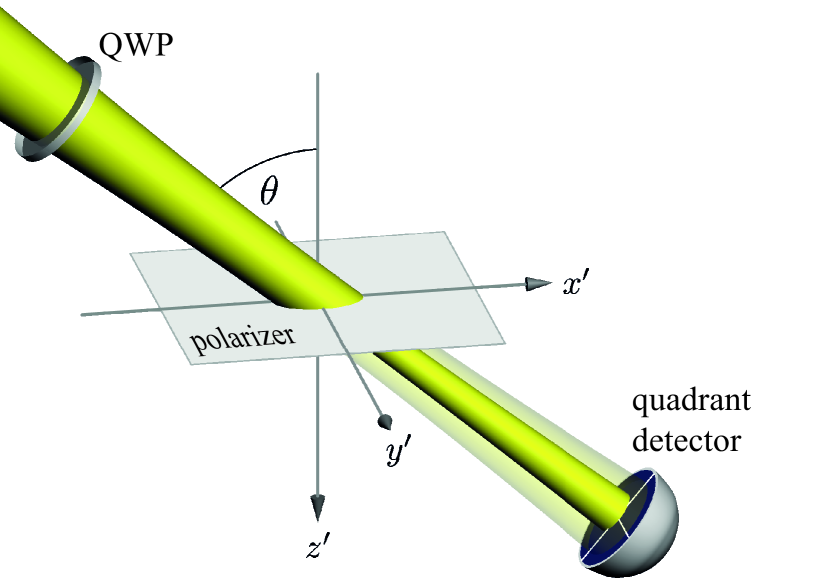
Figure 1: Pictorial representation of the geometric SHEL. After the quarter wave-plate (QWP) the beam is circularly polarized and passes through a polarizer tilted by an angle $\theta$. The center of the intensity distribution of the transmitted beam appears shifted with respect to the axis of the incident beam. Such a shift can be measured by a quadrant detector put behind the polarizer. The reference frame $\{\bm{x}^{\prime},\bm{y}^{\prime},\bm{z}^{\prime}\}$ is aligned with the polarizer surface.

Although the resulting phenomena essentially depend on the type of the interaction with the surface Bekshaev et al. (2011), there are some common characteristics that reveal universality in SOI of light due to the geometry and the dynamical angular momentum aspects of the problem. Amongst the various observable effects resulting from the beam-surface interaction, the so-called geometric Hall effect of light is virtually independent from the properties of the surface Aiello et al. (2009a); Korger et al. (2011); Bekshaev (2009); Bliokh and Nori (2012) and, therefore, represents the ideal candidate for studying above-mentioned universal features. It amounts to a shift of the centroid of the intensity distribution represented by Poynting-vector flow of the beam across the oblique surface of a tilted detector. Direct observation of this effect as originally proposed depends critically on the detector’s response to the light field. However, the question whether the response function of a real detector is indeed proportional to the Poynting vector density is subject to a long-standing debate Berry (2009); Durnin et al. (1981); Braat et al. (2007).

In this work, we implement an alternative scheme Korger et al. (2011), in which the occurrence of the beam shift is independent of the detector response. To this end, we send a circularly polarized beam of light across a tilted polarizing interface to demonstrate a novel kind of geometric Hall effect, in which the centroid of the resulting linearly polarized transmitted beam undergoes a spin-induced transverse shift up to several wavelengths. This is a spatial shift, which is independent of the distance the beam propagated after interaction with the polarizer. Our approach is different from the early proposal Aiello et al. (2009a) in that it is observable with standard optical detectors. Furthermore, it is different from the SHEL occurring in a beam passing through an air-glass interface Hosten and Kwiat (2008) since this geometric SHEL is practically independent of Snell’s law and the Fresnel formulas for the interface.

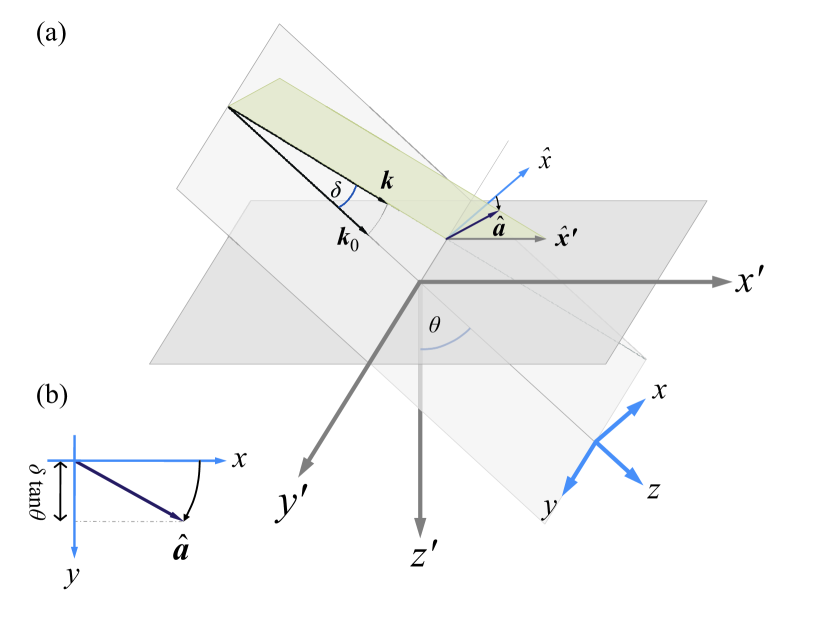
Figure 2: The geometric SHEL at a polarizing interface. (a) The horizontal dark grey plane represents the polarizing interface with the Cartesian reference frame $\{\bm{x}^{\prime},\bm{y}^{\prime}\equiv\bm{y},\bm{z}^{\prime}\}$ attached to it. The axis $\bm{\hat{x}}^{\prime}$ is taken parallel to the absorbing axis of the polarizing interface. $\theta\in[0,\pi/2)$ denotes the angle of incidence. The central wave vector $\bm{k}_{0}$ of the incident beam defines the direction of the axis $\bm{\hat{z}}$ of the frame $\{\bm{x},\bm{y},\bm{z}\}$ attached to the beam. It is instructive to study a wave vector $\bm{k}$ in the $z$-$y$-plane, rotated by an angle $\delta\ll 1$ with respect to $\bm{k}_{0}$. (b) The unit vector $\hat{\bm{a}}\perp\bm{k}$, representing the direction of the absorbed component of the incident field, lies in the common plane of $\bm{k}$ and $\bm{\hat{{x}}}^{\prime}$ (coloured light brown in the figure) and can be obtained, in the first-order approximation, from the rotation by the angle $\delta\tan\theta$ around $\bm{k}$, of the unit vector $\bm{\hat{{x}}}$.

As for conventional SHEL, the physical origin of this geometric version resides in the SOI of light. In fact, we can describe this effect in terms of the geometric phase generated by the spin-orbit interaction as follows: Think of the monochromatic beam as a superposition of many interfering plane waves with the same wavelength and different directions of propagation. When the beam passes through the polarizing interface, the plane wave components with different orientations of their wave vectors acquire different geometric phases determined by distinct local projections yielding to effective “rotations” of the polarization vector around the wave vector. The interference of these modified plane waves produces a redistribution of the intensity spatial profile of the beam resulting in a spin-dependent transverse shift of the intensity centroid.

This effect can be better understood with the help of Figure 2 that illustrates the geometry of the problem. The incident monochromatic beam is made of many plane wave components with wave vectors $\bm{k}$ spreading around the central one $\bm{k}_{0}=k\bm{\hat{{z}}}$, which represents the main direction of propagation of the beam, where $|\bm{k}_{0}|=k=|\bm{k}|$. For a well-collimated beam, the angle $\delta$ between an arbitrary wave vector $\bm{k}$ and the central one $\bm{k}_{0}$ is, by definition, small: $\delta\ll 1$. In the first-order approximation with respect to $\delta$, we consider $\bm{k}=k(\bm{\hat{{z}}}\cos\delta-\bm{\hat{{y}}}\sin\delta)\cong k(\bm{\hat{{z}}}+\kappa_{y}\,\bm{\hat{{y}}})$, where $\kappa_{y}\equiv k_{y}/k=-\sin\delta\cong-\delta$. This wave vector is not the most general one, but, due to the transverse nature of the phenomenon, it is sufficient to restrict the discussion to wave vectors lying in the $yz$ plane. The either left- ($\sigma=+1$) or right-handed ($\sigma=-1$) circular polarization of the incident beam is determined by the unit vector $\bm{\hat{{u}}}_{\sigma}=(\bm{\hat{{x}}}+i\sigma\bm{\hat{{y}}})/\sqrt{2}$ globally defined with respect to the axis $\bm{\hat{z}}$ of the beam frame $\{\bm{\hat{x}},\bm{\hat{y}},\bm{\hat{z}}\}$. However, from Maxwell’s equations it follows that the divergence of the electric field of a light wave in vacuum must vanish. This requires that the polarization vector $\bm{\hat{{e}}}_{\sigma}(\bm{k})$ attached to each plane wave of wave vector $\bm{k}$ must necessarily be transverse, namely $\bm{k}\cdot\bm{\hat{{e}}}_{\sigma}(\bm{k})=0$. This requirement is clearly not satisfied by $\bm{\hat{{u}}}_{\sigma}$ for which one has $\bm{k}\cdot\bm{\hat{{u}}}_{\sigma}/k\cong i\sigma\kappa_{y}/\sqrt{2}\neq 0$. Anyhow, the correct expression for the polarization vector can be easily found by subtracting from $\bm{\hat{{u}}}_{\sigma}$ its longitudinal component: $\bm{\hat{{u}}}_{\sigma}\rightarrow\bm{\hat{{e}}}_{\sigma}(\bm{k})\propto\bm{\hat{{u}}}_{\sigma}-\bm{k}\left(\bm{k}\cdot\bm{\hat{{u}}}_{\sigma}\right)/k^{2}\cong\bm{\hat{{u}}}_{\sigma}-(i\sigma\,\kappa_{y}/\sqrt{2})\bm{\hat{{z}}}$. Now that we have properly modeled the polarization of the incident field, let us see how it changes when the beam crosses the polarizing interface.

A linear polarizer is an optical device that absorbs radiation polarized parallel to a given direction, say $\bm{\hat{x}}^{\prime}$, and transmits radiation polarized perpendicular to that direction. The electric field of each plane wave component of the beam sent through the polarizing interface, changes according to the projection rule $\bm{\hat{e}}_{\sigma}(\bm{k})\rightarrow{\bm{\hat{e}}_{\sigma}(\bm{k})-\bm{\hat{{a}}}(\bm{\hat{{a}}}\cdot\bm{\hat{e}}_{\sigma}(\bm{k}))}=\bm{\hat{{t}}}(\bm{\hat{{t}}}\cdot\bm{\hat{e}}_{\sigma}(\bm{k}))$, where $\bm{a}=\bm{\hat{{x}}}^{\prime}-\bm{k}(\bm{k}\cdot\bm{\hat{x}}^{\prime})/k^{2}$ is the effective absorbing axis with $\bm{\hat{{a}}}=\bm{a}/|\bm{a}|\cong\bm{\hat{{x}}}-\bm{\hat{{y}}}\,\kappa_{y}\tan\theta$, and $\bm{\hat{t}}=\bm{\hat{a}}\times\bm{k}/k$ is the effective transmitting axis. The amplitude of the transmitted plane wave is $\bm{\hat{{t}}}\cdot\bm{\hat{{e}}}_{\sigma}(\bm{k})\propto(1-i\sigma\kappa_{y}\tan\theta)/\sqrt{2}\cong\exp(-i\sigma\kappa_{y}\tan\theta)/\sqrt{2}$, where an irrelevant $\kappa_{y}$-independent overall phase factor has been omitted. Therefore, as a result of the transmission, the amplitude of each plane wave component is reduced by a factor $1/\sqrt{2}$ and multiplied by the geometric phase term $\exp(-i\sigma\kappa_{y}\tan\theta)$. Here, the “$\tan\theta$” behavior of the phase, characteristic of the geometric SHEL Aiello et al. (2009a), is in striking contrast to the typical “$\cot\theta$” angular dependence of the conventional SHEL as, e. g., the Imbert-Fedorov shift Liu and Li (2008). However, the spin-orbit interaction term $\sigma\kappa_{y}$, expressing the coupling between the spin $\sigma$ and the transverse momentum $\kappa_{y}$ of the beam, is characteristic of both phenomena, thus revealing their common physical origin.

According to the Fourier transform shift theorem Goodman (2005), a linear phase shift in the wave vector domain introduces a translation in the space domain. Using this theorem, we can show that the geometric phase term $\exp(-i\sigma\kappa_{y}\tan\theta)$ leads to a beam shift along the $\bm{\hat{y}}$-direction. This can be explicitly demonstrated by writing the incident circularly polarized paraxial beam as $\bm{\Psi}^{\text{in}}(y)=\bm{\hat{{u}}}_{\sigma}\psi_{\sigma}^{\text{in}}(y)$, where only the dependence on the relevant transverse coordinate $y$ has been displayed. With $\widetilde{\psi}_{\sigma}^{\text{in}}(\kappa_{y})$ we denote the Fourier transform of $\psi_{\sigma}^{\text{in}}(y)$. The two functions are connected by the simple relation $\psi_{\sigma}^{\text{in}}(y)=\int\widetilde{\psi}_{\sigma}^{\text{in}}(\kappa_{y})\exp(ik\kappa_{y}y)\text{d}\kappa_{y}$. After transmission across the polarizing interface, the Fourier transform $\widetilde{\psi}_{\sigma}^{\text{in}}(\kappa_{y})$ of $\psi_{\sigma}^{\text{in}}(y)$ changes to $\widetilde{\psi}_{\sigma}^{\text{in}}(\kappa_{y})\linebreak[1]\exp(-i\sigma\kappa_{y}\tan\theta)\linebreak[1]/{\sqrt{2}}$ and the output field can be written as

$$\psi_{\sigma}^{\text{out}}(y) =\frac{1}{\sqrt{2}}\int\widetilde{\psi}_{\sigma}^{\text{in}}(\kappa_{y})\exp[ik\kappa_{y}(y-\sigma\tan\theta/k)]\text{d}\kappa_{y}$$

$$=\frac{1}{\sqrt{2}}\psi_{\sigma}^{\text{in}}(y-\sigma\tan\theta/k)\text{.}$$ (1)

This last expression clearly shows that the scalar amplitude of the output field is equal, apart from the $1/\sqrt{2}$ factor, to the amplitude of the input field transversally shifted by $\sigma\tan\theta/k$. Finally, the position of the centroid of the transmitted beam is given by

$$\langle y\rangle=\frac{\int y\,|\psi_{\sigma}^{\text{out}}(y)|^{2}\text{d}y}{\int|\psi_{\sigma}^{\text{out}}(y)|^{2}\text{d}y}=\frac{\sigma}{k}\tan\theta\text{,}$$ (2)

where $k=\frac{2\pi}{\lambda}$.

Eq. (2) as derived above is valid for an ideal polarizer with a high extinction ratio. In this case, the description of the polarizer as a projection onto the effective transmission axis $\bm{\hat{t}}$ is adequate. At normal incidence ($\theta=0$) such polarizers are readily available. However, working with tilted polarizing interfaces, we have to account for the fact that the efficiency of the polarizer diminishes with larger angles $\theta$. As a result of such loss of efficiency, the “$\tan\theta$”-dependence of the shift is modified as illustrated in Fig. 5. This is explained in detail in the Supplemental Material, where we introduce a phenomenological model for our real-world polarizer Fainman and Shamir (1984); Korger et al. (2013); Haus (1993); Aiello et al. (2009b); Hung-Chia and Jing-Ren (1983); Hsu et al. (2004).

In the experiment, we use a Corning Polarcor polarizer, made of two layers of elongated and oriented silver nano-particles embedded in a $$25\text{\,}\mathrm{mm}$\times$25\text{\,}\mathrm{mm}$\times$0.5\text{\,}\mathrm{mm}$$ glass substrate. Directed absorption from these particles effectively polarizes the transmitted beam. In order to avoid parasitic effects from the glass surfaces ($n_{G}=1.517$), we have submerged the polarizer in a tank with index matching liquid (Cargille laser liquid 5610, $n_{L}=1.521$). Without this liquid, the effective tilting angle inside the glass polarizer would be limited by Snell’s law to $\arcsin(1/n_{G})\approx 41$.

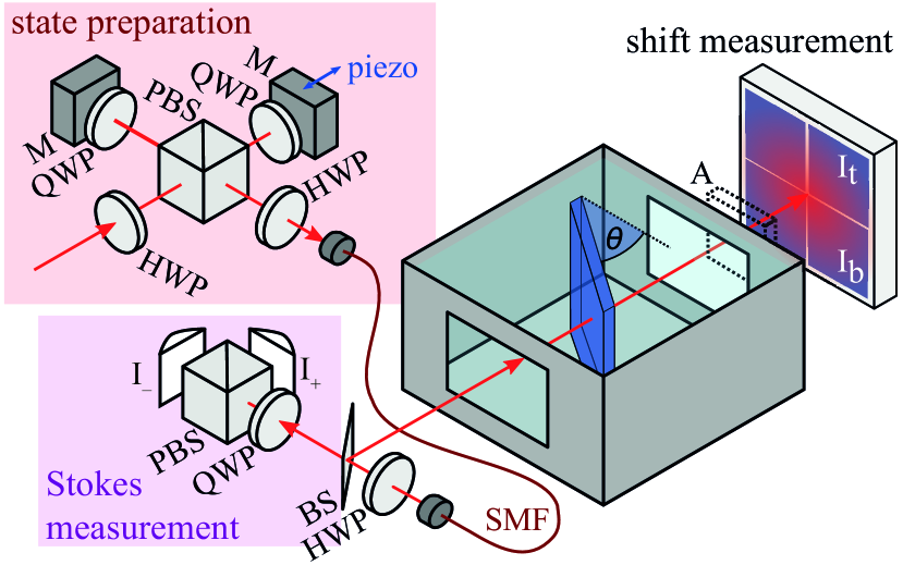
Figure 3: Experimental Setup: Simultaneous measurement of the incident state of polarization and the position of a light beam transmitted across a tilted polarizer. State preparation: The relative phase between horizontally and vertically polarized components is modulated using a polarizing beam splitter (PBS), a piezo mirror (M), quarter and half wave plates (QWP, HWP). The beam is spatially filtered using a single-mode fibre (SMF). Stokes measurement: The transmitted port of a beam splitter (BS) is used to monitor the state of polarization. We use the Stokes parameters $S_{3}$ to distinguish left- and right-hand circular polarization. Shift measurement: The beam is propagated across our sample, a tank containing a glass polarizer and an index-matching liquid, and its position is observed using a quadrant detector. An optional PBS (A) can be employed as an analyzer in front of the detector. The photo currents $I_{+}$, $I_{-}$, $I_{t}$, and $I_{b}$ are amplified and digitally sampled for 1  at 50 .

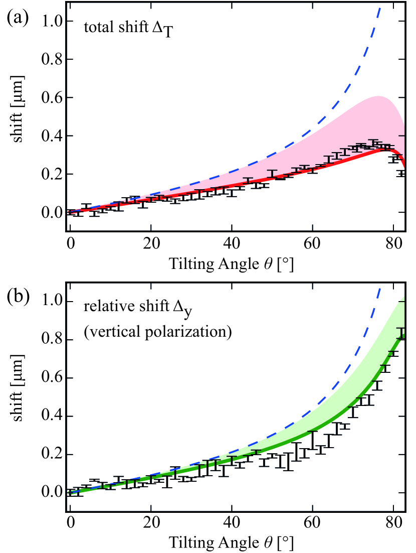
Figure 4: Polarization-dependent beam shifts occurring at a tilted polarizer. Measurement data and theoretical predictions are shown. Both series of shift measurements were repeated five times. We report the mean value and standard deviation of the mean. The dashed blue line shows the theory for a perfect polarizer, while the shaded area indicates the result of our phenomenological polarizer model for a reasonable range of parameters. Details are given in the SM. (a) Overall displacement $\Delta_{T}$ of the intensity barycentre after transmission across the polarizer. (b) Displacement $\Delta_{y}$ of the vertically polarized intensity component solely. The two measurements $\Delta_{T}$ and $\Delta_{y}$ differ due to the imperfect nature of our polarizer as discussed in the SM.

In our setup (Figure 3), a fundamental Gaussian light beam ($\lambda=$795\text{\,}\mathrm{nm}$$) is prepared with the state of polarization alternating between left- and right-hand circular. To avoid spatial jitter, the spatial mode is cleaned using a single mode fibre and no active elements are used after the fibre. We collimate the light beam using an aspheric lens (New Focus 5724-H-B) aligned such that the beam waist is at the position of the detector.

In order to simultaneously measure the beam position $\big{\langle}y{}\big{\rangle}$ and the incident state of polarization, we employ a dielectric mirror (Layertec 103210) as a non-polarizing beam splitter at an angle of incidence of $3$. The reflected and transmitted states of polarization coincide within experimental accuracy. The beam centroid $\big{\langle}y{}\big{\rangle}=f\frac{I_{t}-I_{b}}{I_{t}-I_{b}}$ and Stokes parameter $S_{3}=\frac{I_{+}-I_{-}}{I_{+}+I_{-}}$ are calculated from the digitized photo currents. We can measure the calibration factor $f$ in-situ by translating the quadrant detector using a micrometre stage.

Since the signal is periodic with the modulation frequency $f_{\text{mod}}=29\,$, we can filter technical noise in a post-processing stage. To this end, the discrete Fourier transform is computed and only spectral components with frequencies equal to $f_{\text{mod}}$ and higher harmonics thereof are passed.

We identify $S_{3}=0.99\pm 0.01$ and $S_{3}=-0.99\pm 0.01$ with the circular states of polarization $\sigma=+1$ and $\sigma=-1$ respectively. For both states, we calculate the mean of all corresponding beam positions $\big{\langle}y{}\big{\rangle}\left(\sigma\right)$ and the helicity-dependent displacement $\Delta^{\mathrm{R}}=\big{\langle}y{}\big{\rangle}\left({\sigma=+1}\right)-\big{\langle}y{}\big{\rangle}\left(\sigma=-1\right)$.

An extensive characterization of statistical and systematic errors revealed that the observed position of the light beam depends slightly on the state of polarization even if no sample is present in the beam path. The magnitude of this spurious beam shift is typically much smaller than the phenomenon, we intend to study. In the Supplemental material, we discuss that this amounts to a small offset (60 nm) on the raw data points $\Delta^{\mathrm{R}}(\theta)$, independent from the action of the sample. Thus, the shift measurements $\Delta(\theta)=\Delta^{\mathrm{R}}(\theta)-\Delta^{\mathrm{R}}(0)$ reported here are corrected with respect to the raw data.

We investigate beam shifts in two different configurations. First, we measure the displacement $\Delta_{T}=2\big{\langle}y{}\big{\rangle}_{{|\bm{E}_{T}|^{2}}}$ of the total transmitted energy density distribution $|\bm{E}_{T}|^{2}$ when switching the incident state of polarization from $\sigma=+1$ to $\sigma=-1$ (Figure 4(a)). Then, we employ an additional polarization analyzer in front of the detector and observe the shift $\Delta_{y}=2\big{\langle}y{}\big{\rangle}_{{|E_{{y}}|^{2}}}$ of the energy density $|E_{y}|^{2}=|\bm{E}_{T}\cdot\bm{\hat{y}}|^{2}$ of the vertically polarized field component solely (Figure 4(b)). These variants of the experiment coincide for polarizers with perfect extinction ratios but can differ significantly for real-world polarizers with minor deficiencies.

The beam shift observed in the latter case increases proportionally to the tangent of the tilting angle, exceeding one wavelength. This characteristic “$\tan\theta$”-behaviour (and “real-world-polarizer” modification thereof) is unique to the geometric spin Hall effect of light. In both cases, the measurement agrees well with theoretical predictions using our phenomenological model.

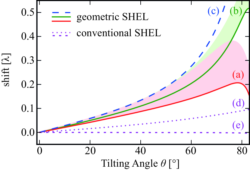
Figure 5: Theory for the conventional spin Hall effect of light compared to the geometric SHEL. A light beam transmitted across an interface between two media can undergo a transverse displacement known as the Imbert-Fedorov effect or conventional SHEL. Here, we plot this displacement for a left-hand circularly polarized beam ($\sigma=+1$) for two different cases and compare this with the geometric SHEL studied in this work. (a) and (b) Geometric SHEL $\frac{1}{2}\Delta_{T}$ and $\frac{1}{2}\Delta_{y}$ for the same configuration as in Figure 4. (c) Geometric SHEL as predicted for an ideal polarizing interface. (d) Conventional SHEL occurring at an air-glass interface ($n_{1}=1$, $n_{2}=1.5$). (e) Conventional SHEL expected for the entrance face of our submerged polarizer ($n_{1}=n_{L}=1.521$, $n_{2}=n_{G}=1.517$).

To the best of our knowledge, this is the first direct measurement of this intriguing phenomenon. The geometric spin Hall effect of light should not be confused with the conventional SHEL or Imbert-Fedorov shift. The latter occurs at a physical interface and, while such interfaces are present in our experimental setup, they can only give rise to beam shifts significantly smaller than the observed effect. In Figure 5, we compare our results to the Imbert-Fedorov shift, which could occur at the polarizer substrate, for a set of realistic parameters Bliokh and Bliokh (2006); Liu and Li (2008). This illustrates that the beam shifts measured in this work constitute a novel spin Hall effect of light, virtually independent from surface effects.

In conclusion, we have demonstrated the geometric spin Hall effect of light experimentally by propagating a circularly polarized laser beam across a suitable polarizing interface. The centre of mass of the transmitted light field was found to be displaced with respect to position of the incident beam as predicted by the theory. While a Gaussian light beam itself is invariant with respect to rotation around its axis of propagation, the geometry induced by the tilted polarizer, breaks this symmetry. The resulting displacement can be interpreted as a spin-to-orbit coupling characteristic for spin Hall effects of light.

Supplemental Material

.1 Phenomenological polarizer model and characterization of our real-world polarizer

In this section, we describe a geometric polarizer model, analogously to the work by Fainman and Shamir Fainman and Shamir (1984), and determine empirical parameters relevant for the actual polarizer used in our experiment. Here, the interaction of an arbitrarily oriented polarizer with a plane wave is discussed while we deal with real light beams in the subsequent section on beam shifts.

A polarizer is an optical device that alters the state of polarization and intensity of a plane wave without effecting its direction of propagation $\bm{\hat{\kappa}}=\bm{k}/k$. The polarizer used within this work can be described by a real-valued unit vector $\bm{\hat{P}}_{a}$ describing its absorbing axis. Projecting $\bm{\hat{P}}_{a}$ onto the transverse plane of the electric field yields an effective absorbing axis

$$\bm{\hat{a}}(\bm{\hat{\kappa}})=\frac{\bm{\hat{P}}_{a}-(\bm{\hat{P}}_{a}\cdot\bm{\hat{\kappa}})\,\bm{\hat{\kappa}}}{\sqrt{1-(\bm{\hat{P}}_{a}\cdot\bm{\hat{\kappa}})^{2}}}\text{.}$$ (S1)

Thus, the electric field transmitted across an idealized polarizer is

$$\bm{\tilde{E}}_{T}=\bm{\tilde{E}}_{I}-\bm{\hat{a}}\left(\bm{\hat{a}}\cdot\bm{\tilde{E}}_{I}\right)=\bm{\hat{t}}\left(\bm{\hat{t}}\cdot\bm{\tilde{E}}_{I}\right)\text{,}$$ (S2)

where $\bm{\tilde{E}}_{I}=\bm{\tilde{E}}_{I}(\bm{k})$ is the amplitude of the plane wave $\exp(i\,\bm{\hat{\kappa}}\cdot\bm{r})$, and

$$\bm{\hat{t}}(\bm{\hat{\kappa}})=\bm{\hat{a}}(\bm{\hat{\kappa}})\times\bm{\hat{\kappa}}=\frac{\bm{\hat{P}}_{a}\times\bm{\hat{\kappa}}}{|\bm{\hat{P}}_{a}\times\bm{\hat{\kappa}}|}$$ (S3)

is the effective transmitting axis.

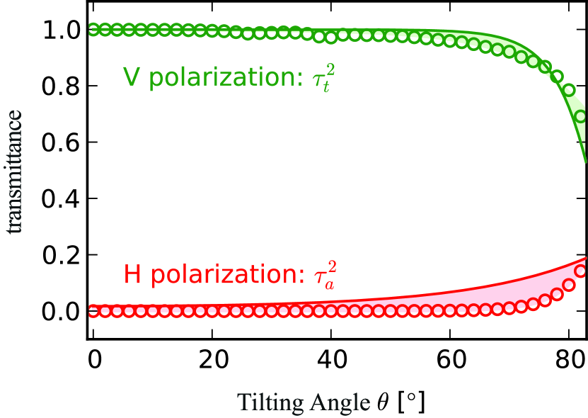
Figure S1: Transmittance of light beams across the polarizer as a function of the tilting angle $\theta$ and the incident state of polarization. The polarizer is aligned such that at normal incidence ($\theta=0$), vertical (V) polarization is transmitted and horizontal (H) polarization is blocked. We observe how the transmittance changes when the polarizer is rotated around the vertical axes and compare the experimental data (circles) to our phenomenological model (S4) for different parameters $\tau_{t}$ and $\tau_{a}$. The shaded regions indicate the range of parameters considered within this work. One limit (S6) is depicted with solid lines and shows the best fit with the observed beam shifts. The other limit is the best fit to the measured transmittances.

However, real-world polarizers have finite extinction ratios and an experimental characterization shows that the effectiveness of our polarizer decreases when tilted (Figure S1). Thus, we have found it convenient to phenomenologically describe the transmitted light field as

$$\bm{\tilde{E}}_{T}=\tau_{t}\,\bm{\hat{t}}\left(\bm{\hat{t}}\cdot\bm{\tilde{E}}_{I}\right)+\tau_{a}\,\bm{\hat{a}}\left(\bm{\hat{a}}\cdot\bm{\tilde{E}}_{I}\right)\text{.}$$ (S4)

Here, we employ two empirical parameters, $\tau_{a}(\theta)$ and $\tau_{t}(\theta)$, depending on the angle $\theta$ between the propagation direction $\bm{\hat{\kappa}}$ and the unit vector perpendicular to the surface of the polarizer. We have found the following set of parameters to be in very good agreement with the observed transmission:

$$\tau_{t}(\theta) =1-0.31\,\exp(-5.6\,\cos\theta)$$ (S5a)

$$\tau_{a}(\theta) =0.93\,\exp(-6.4\,\cos\theta)$$ (S5b)

This simple model is sufficient for our purpose, albeit it does not describe the complex behaviour of the polarizer perfectly. A more detailed study of tilted polarizers can be found in Ref. Korger et al. (2013).

In the following section, we will use this model to calculate beam shifts. We have shown in the main text (Fig. 4), that this prediction matches qualitatively to our observation. Since the magnitude of these beam shifts depend critically on the parameters $\tau_{t}$ and $\tau_{a}$, a slightly different choice significantly increases the quantitative agreement:

$$\tau_{t}(\theta) =1-1.2\,\exp(-12\,\cos\theta)$$ (S6a)

$$\tau_{a}(\theta) =0.51\,\exp(-1.3\,\cos\theta)$$ (S6b)

These parameters can be found by a combined fit of both, the observed transmission and the beam shifts. In figures 4, 5, and S1, the latter choice (S6) is depicted using thick solid lines. Shaded regions indicate a range of realistic parameters including both (S5) and (S6) as limits.

.2 Calculation of beam shifts occurring at an oblique polarizer according to our phenomenological model

In this section, we adapt the theory for the geometric spin Hall effect of light originally calculated for a different type of polarizer Korger et al. (2011) to our phenomenological model. To this end, we express the polarizer’s absorbing axis

$$\bm{\hat{P}}_{a}=\bm{\hat{x}}^{\prime}=\cos\theta\,\bm{\hat{x}}+\sin\theta\,\bm{\hat{z}}$$ (S7)

in the global reference frame $\{\bm{\hat{x}},\bm{\hat{y}},\bm{\hat{z}}\}$, aligned with the direction $\bm{\hat{z}}$ of beam propagation.

The incident beam $\bm{E}_{I}(\bm{r})$ is circularly polarized and well-collimated, i.e. it has a low divergence $\theta_{0}$, with a Gaussian transverse intensity profile. This is expanded in a plane wave basis with amplitudes $\bm{\tilde{E}}_{I}(\bm{\hat{\kappa}})$ such that the $\bm{\hat{\kappa}}$-dependent projection (S4) can be applied.

As a consequence of our polarizer model, the electric field $\bm{E}_{T}(\bm{r})$ after transmission across such a polarizer, is a superposition of two orthogonally polarized field components, $\bm{E}_{x}(\bm{r})$ and $\bm{E}_{y}(\bm{r})$. Thus, the electric field energy density distribution (at the detection plane $z=0$)

$$\begin{split}|\bm{E}_{T}(x,y)|^{2}&=\underbrace{|\bm{E}_{T}\cdot\bm{\hat{x}}|^{2}}_{=|E_{x}|^{2}}+\underbrace{|\bm{E}_{T}\cdot\bm{\hat{y}}|^{2}}_{=|E_{y}|^{2}}+\underbrace{|\bm{E}_{T}\cdot\bm{\hat{z}}|^{2}}_{\approx 0}\end{split}$$ (S8)

can be decomposed analogously.

Geometric SHEL manifests itself as a transverse displacement $\big{\langle}y{}\big{\rangle}$ of the transmitted light beam’s barycentre. The total electric energy density $|\bm{E}_{T}|^{2}$ and both of its non-vanishing components undergo such a shift. Since this spatial displacement is independent from the $z$ coordinate, we restrict the discussion to the detection plane at $z=0$. It is convenient to write the total energy density’s barycentre

$$\big{\langle}y{}\big{\rangle}_{{|\bm{E}_{T}|^{2}}}=w_{x}\,\big{\langle}y{}\big{\rangle}_{{|E_{{x}}|^{2}}}+w_{y}\,\big{\langle}y{}\big{\rangle}_{{|E_{{y}}|^{2}}}$$ (S9)

as a weighted sum of the relative shifts occurring for the horizontally and vertically polarized components respectively. Here,

$$\big{\langle}y{}\big{\rangle}_{{u}}=\frac{\iint\limits y\,u(x,y)\operatorname{d}x\operatorname{d}y}{\iint\limits u(x,y)\operatorname{d}x\operatorname{d}y}$$ (S10)

denotes the centre of mass along the $\bm{\hat{y}}$ direction calculated with respect to a scalar distribution $u(x,y)$. The integration spans the whole detection plane.

The weights

$$\begin{split}w_{x}(\theta)&=\frac{\iint\limits E_{x}^{2}(x,y)\operatorname{d}x\operatorname{d}y}{\iint\limits|\bm{E}|^{2}(x,y)\operatorname{d}x\operatorname{d}y}\\ &=\frac{\tau_{a}^{2}(\theta)}{\tau_{a}^{2}(\theta)+\tau_{t}^{2}(\theta)}+\mathcal{O}(\theta_{0}^{2})\quad\text{ and}\end{split}$$ (S11)

$$w_{y}(\theta) =\frac{\tau_{t}^{2}(\theta)}{\tau_{a}^{2}(\theta)+\tau_{t}^{2}(\theta)}+\mathcal{O}(\theta_{0}^{2})$$ (S12)

introduced in (S9) depend on the empirical parameters $\tau_{t}$ and $\tau_{a}$ (S6). Finally, we can calculate the relative shifts

$$\begin{split}\frac{\big{\langle}y{}\big{\rangle}_{{|E_{{i}}|^{2}}}}{\lambda}&=\frac{\iint\limits_{x,y}y\,|E_{{i}}|^{2}\operatorname{d}x\operatorname{d}y}{\iint\limits_{x,y}\,|E_{{i}}|^{2}\operatorname{d}x\operatorname{d}y}\\ &=\sigma\,\frac{\tan\theta}{2\,\pi}\,f_{i}(\theta)+\mathcal{O}(\theta_{0}^{2})\text{,}\end{split}$$ (S13)

where the factors

$$f_{x}(\theta) =1-\frac{\tau_{t}(\theta)}{\tau_{a}(\theta)}<0\quad\text{ and}$$ (S14a)

$$f_{y}(\theta) =1-\frac{\tau_{a}(\theta)}{\tau_{t}(\theta)}>0$$ (S14b)

depend critically on the performance of the polarizer.

Note that, since the transmission coefficients are real and positive and $1\geq\tau_{t}>\tau_{a}$ (Figure S1), these relative shifts have opposite signs. Consequently, the displacement of the total energy density

$$\frac{\big{\langle}y{}\big{\rangle}_{{|\bm{E}_{T}|^{2}}}}{\lambda}=\sigma\,\frac{\tan\theta}{2\,\pi}\,\underbrace{\left(w_{x}\,f_{x}+w_{y}\,f_{y}\right)}_{<1}$$ (S15)

is smaller than the relative shift $\big{\langle}y{}\big{\rangle}_{{|E_{{y^{\prime}}}|^{2}}}$ of the vertically polarized component solely. For our realistic polarizer model, both shifts are smaller than expected for the ideal case. This matches very well with our experimental observation.

For a perfect polarizer with $\tau_{a}=0$ and $\tau_{t}=1$, equation (S15) reduces to eq. (2) since $w_{x}\,f_{x}=\frac{\tau_{a}^{2}}{\tau_{t}^{2}}\left(1-\frac{\tau_{t}}{\tau_{a}}\right)\rightarrow 0$ for $\tau_{a}\rightarrow 0$. This is exactly the same expression that was originally found for the polarizer model by Fainman and Shamir Korger et al. (2011).

.3 Calculation of the geometric spin Hall effect of light at a polarizing interface

In this part, we derive detailed eq. (2) for a paraxial fundamental Gaussian beam incident at an angle $\theta$ upon the surface of an absorbing polarizer whose absorbing axis is directed along $x^{\prime}$. The Cartesian coordinate systems attached to the polarizing interface and to the beam are still defined as in Fig. 2A in the main text. However, now the axis $x^{\prime}$ is taken parallel to the absorbing axis of the polarizer, in order to reproduce the actual experimental conditions.

Consider the fundamental solution of the scalar paraxial wave equation Goodman (2005) that we indicate with $\psi(\bm{r})$:

$$\psi(\bm{r})=\left(\frac{k}{\pi L}\right)^{1/2}\frac{i}{1+iz/L}\exp\left(-\frac{1}{w_{0}^{2}}\frac{x^{2}+y^{2}}{1+iz/L}\right),$$ (S16)

where the Rayleigh range $L$ of the beam can be expressed in terms of the beam waist $w_{0}$ as $L=kw_{0}^{2}/2$, with $\theta_{0}=2/(kw_{0})\ll 1$ denoting the angular spread of the beam. In the first-order approximation with respect to $\theta_{0}$, the electric vector field of the incident beam can be written as Haus (1993):

$$\bm{\Psi}^{\text{in}}(\bm{r}) =\bm{\hat{u}}_{\sigma}\,\psi(\bm{r})+\bm{\hat{z}}\frac{i}{k}\bm{\hat{u}}_{\sigma}\cdot\bm{\nabla}\psi(\bm{r})$$

$$=\left[\bm{\hat{u}}_{\sigma}-i\bm{\hat{z}}\frac{\theta_{0}\,(x+i\sigma y)}{\sqrt{2}\,w_{0}\,(1+iz/L)}\right]\psi(\bm{r})\text{,}$$ (S17)

where $\hat{\bm{u}}_{\sigma}=(\hat{\bm{x}}+i\sigma\hat{\bm{y}})/\sqrt{2}$ and an overall (irrelevant) multiplicative term has been omitted. In Ref. Aiello et al. (2009b) it was demonstrated that the field transmitted by an arbitrarily oriented polarizer can be written as a perturbative expansion of the form

$$\begin{split}\bm{\Psi}^{\text{out}}(\bm{r})=&\;\widetilde{G}_{00}\bm{\Psi}^{\text{in}}(\bm{r})\\ &-\frac{i}{k}\left[\widetilde{G}_{10}\frac{\partial\bm{\Psi}^{\text{in}}}{\partial x}(\bm{r})+\widetilde{G}_{01}\frac{\partial\bm{\Psi}^{\text{in}}}{\partial y}(\bm{r})\right]\\ &+O(\theta_{0}^{2}),\end{split}$$ (S18)

where the $3\times 3$ matrices $\widetilde{G}_{nm}$ are defined as

$$\widetilde{G}_{nm}=\left.\frac{k^{n+m}}{n!m!}\frac{\partial^{n+m}(\hat{\bm{n}}\hat{\bm{n}})}{\partial k_{x}^{n}\partial k_{y}^{m}}\right|_{k_{x}=0,\;k_{y}=0}.$$ (S19)

For our absorbing polarizer, the dyadic form

$$\bm{\hat{n}}\bm{\hat{n}}=\left(\begin{array}[]{ccc}n_{x}^{2}&n_{x}\,n_{y}&n_{x}\,n_{z}\\ n_{y}\,n_{x}&n_{y}^{2}&n_{y}\,n_{z}\\ n_{z}\,n_{x}&n_{z}\,n_{y}&n_{z}^{2}\end{array}\right)$$ (S20)

is defined in terms of the effective-transmission unit vector $\bm{\hat{{n}}}=\bm{\hat{{a}}}\times\bm{\hat{{\kappa}}}=n_{x}\bm{\hat{x}}+n_{y}\bm{\hat{y}}+n_{z}\bm{\hat{z}}$, where

$$\hat{\bm{a}}=\frac{\hat{\bm{x}}^{\prime}-\hat{\bm{\kappa}}(\hat{\bm{\kappa}}\cdot\hat{\bm{x}}^{\prime})}{\sqrt{1-|\hat{\bm{\kappa}}\cdot\hat{\bm{x}}^{\prime}|^{2}}},$$ (S21)

and $\hat{\bm{\kappa}}=\bm{k}/k$. A straightforward calculation furnishes

$$\widetilde{G}_{00}=\left(\begin{array}[]{ccc}0&0&0\\ 0&1&0\\ 0&0&0\end{array}\right),$$ (S22a)

$$\widetilde{G}_{01}=\left(\begin{array}[]{ccc}0&\tan\theta&0\\ \tan\theta&0&-1\\ 0&-1&0\end{array}\right)\text{,}$$ (S22b)

$$\widetilde{G}_{10}=\left(\begin{array}[]{ccc}0&0&0\\ 0&0&0\\ 0&0&0\end{array}\right)\text{.}$$ (S22c)

Substitution of equations (S22) and (.3) into equation (S18) yields to the following first-order expression for the transmitted field:

$$\begin{split}\bm{\Psi}^{\text{out}}(\bm{r})=\frac{\psi(\bm{r})}{\sqrt{2}}\bigg{[}&-\hat{\bm{x}}\,\theta_{0}\frac{y}{w_{0}}\frac{\sigma\tan\theta}{1+iz/L}\\ &+\hat{\bm{y}}\,i\sigma\left(1+\theta_{0}\frac{y}{w_{0}}\frac{\sigma\tan\theta}{1+iz/L}\right)\\ &+\hat{\bm{z}}\,\theta_{0}\frac{y}{w_{0}}\frac{\sigma}{1+iz/L}\bigg{]}+O(\theta_{0}^{2}).\end{split}$$ (S23)

The electric field energy density, the physical quantity actually measured by a standard optical detector, is proportional to $|\bm{\Psi}^{\text{out}}(\bm{r})|^{2}$ which can be calculated from Eq. (S21) as:

$$|\bm{\Psi}^{\text{out}}(\bm{r})|^{2}=|\psi(\bm{r})|^{2}\left(\frac{1}{2}+\theta_{0}\frac{y}{w_{0}}\frac{\sigma\tan\theta}{1+iz/L}\right)+O(\theta_{0}^{2}).$$ (S24)

Finally, the sought shift is calculated as the first moment of the electric field energy density distribution, namely

$$\langle y\rangle= \;\frac{\displaystyle{\int\!\!\!\!\int y\,|\bm{\Psi}^{\text{out}}(\bm{r})|^{2}\text{d}x\text{d}y}}{\displaystyle{\int\!\!\!\!\int|\bm{\Psi}^{\text{out}}(\bm{r})|^{2}\text{d}x\text{d}y}}$$

$$= \;\frac{\sigma}{k}\tan\theta,$$ (S25)

where the integration is evaluated over all the $xy$ plane at $z=0$. Equation (.3) reproduces the result given by eq. (2) in the main text.

.4 Discussion of spurious beam shifts

In our experiment, we prepare left and right circularly polarized Gaussian light beams and intend to study how a sample effects the position of the transmitted beam in both cases. The spatial modes prepared in each case are almost, yet not exactly identical. Despite being filtered using two metres of single-mode fibre, there can be a tiny offset between the centre of mass of the left versus the right circularly polarized beam prepared in this manner. While this effect is too small to be imaged on a CCD camera, it can be revealed in a precision measurement as employed in this work.

Theoretically, we can account for such spurious beam shifts by substituting the ideal Gaussian profile $\bm{\tilde{E}}_{I}(\bm{\hat{\kappa}})$ with a generic paraxial beam such as a power series or superposition of Hermite-Gaussian laser modes. This changes the result (S13) to

$$\frac{\big{\langle}y{}\big{\rangle}_{{|E_{{i}}|^{2}}}}{\lambda}=\sigma\,\frac{\tan\theta}{2\,\pi}\,f_{i}(\theta)+Y_{i}(\sigma)+\mathcal{O}(\theta_{0}^{2})\text{,}$$ (S26)

where $Y_{i}(\sigma)$ is an offset independent of the tilting angle $\theta$, which can also be understood intuitively: The deviation between two almost identical beam profiles amounts to either a spatial or an angular beam shift. First, since the sample is spatially homogeneous, a spatial displacement of the whole beam, does not change the interaction at all. And second, while the interaction with the sample generally depends on the angle of incidence, a slightly different direction of propagation, here on the order of $10^{-6}~{}\rad$, is practically negligible.

In our experiment, we measure the helicity-dependent beam shift

$$\begin{split}\Delta^{\mathrm{R}}&=\big{\langle}y{}\big{\rangle}\left({\sigma=+1}\right)-\big{\langle}y{}\big{\rangle}\left(\sigma=-1\right)\\ &=\underbrace{2\frac{\tan\theta}{2\,\pi}\,f_{i}(\theta)}_{\Delta(\Theta)}+\underbrace{Y_{i}(\sigma=+1)-Y_{i}(\sigma=-1)}_{\Delta^{\mathrm{R}}(\theta=0)}\text{,}\end{split}$$ (S27)

which contains a spurious offset $\Delta^{\mathrm{R}}(\theta=0)\approx 60~{}\nano$. The data shown in Fig. 4 is corrected for this offset.

Such offset can be roughly quantified in a simple manner. In our experimental conditions, the used single-mode fiber does not support exactly a single mode only, namely the fundamental $\text{TEM}_{00}$ mode, but also first-order modes such as $\text{TEM}_{10}$ and $\text{TEM}_{01}$. Ideally, a conventional single-mode optical fiber possesses a simple circular cylindrical geometry in absence of either intentional or accidental deformations of the fiber structure. Any deviations from the ideal configuration causes proliferation of, and coupling between, normal modes of the fiber. Typically, a small coupling may occur because of several reasons, including intrinsic or induced cross-sectional ellipticity, bending, twist, etc., of the fiber cross section Hung-Chia and Jing-Ren (1983). Now, it is well known that the coupling between fundamental and first-order modes causes a shift of the centroid of the intensity distribution of the guided light inside the fiber Hsu et al. (2004). This can be seen by writing the electric field distribution $E(x,y)$ (with a fixed uniform polarization) of the guided light, as a superposition of the $\text{TEM}_{00}$ and the $\text{TEM}_{01}$ mode

$$E(x,y)\approx\text{TEM}_{00}(x,y)+\eta\,\text{TEM}_{01}(x,y),$$ (S28)

where $0<\eta\leq 1$ is the dimensionless coupling parameter. The spatial intensity distribution of such a field configuration is displaced along the $y$-axis by $\Delta y$, where

$$\Delta y= \;\frac{\displaystyle{\iint y\left|E(x,y)\right|^{2}\,\text{d}x\text{d}y}}{\displaystyle{\iint\left|E(x,y)\right|^{2}\,\text{d}x\text{d}y}}$$

$$= \;w_{0}\,\frac{\eta}{1+\eta^{2}}$$

$$\simeq \;w_{0}\,\eta,$$ (S29)

where the last, approximate equality holds in the case $\eta\ll 1$ and $2w_{0}$ is the diameter of the fundamental $\text{TEM}_{00}(x,y)$ mode of the fiber. In our experimental conditions, we had $w_{0}=2.5\,\mu\text{m}$ and we measured $\Delta y\simeq 60\,\text{nm}$. By inserting these values into Eq. (.4) we obtain $\eta\simeq\Delta y/w_{0}\simeq 0.024$. This number tells us that it is enough to have an amplitude ratio of about $2\%$ between the first-order $\text{TEM}_{01}$ and the fundamental $\text{TEM}_{00}$ mode, to observe a transverse shift of $60\,\text{nm}$.

For the present rough estimation, the use of a single scalar coupling coefficient $\eta$ is appropriate. However, if one would adhere more to the physical reality of the phenomenon, one would rather use a tensor coupling coefficient $\eta_{ij}$ in order to account for the polarization-dependence of the coupling.

References

- Goos and Hänchen (1947) F. Goos and H. Hänchen, Ann. Phys. (Leipzig) 436, 333 (1947).
- Fedorov (1955) F. I. Fedorov, Dokl. Akad. Nauk. SSSR 105, 465 (1955).
- Imbert (1972) C. Imbert, Phys. Rev. D 5, 787 (1972).
- Aiello (2012) A. Aiello, New J. Phys. 14, 013058 (2012).
- Pillon et al. (2004) F. Pillon, H. Gilles, and S. Fahr, Appl. Opt. 43, 1863 (2004).
- Ménard et al. (2009) J.-M. Ménard, A. E. Mattacchione, M. Betz, and H. M. van Driel, Opt. Lett. 34, 2312 (2009).
- Merano et al. (2007) M. Merano, A. Aiello, G. W. ’t Hooft, M. P. van Exter, E. R. Eliel, and J. P. Woerdman, Opt. Express 15, 15928 (2007).
- Schilling (1965) H. Schilling, Ann. Phys. (Leipzig) 471, 122 (1965).
- Onoda et al. (2004) M. Onoda, S. Murakami, and N. Nagaosa, Phys. Rev. Lett. 93, 083901 (2004).
- Hosten and Kwiat (2008) O. Hosten and P. Kwiat, Science 319, 787 (2008).
- Yin et al. (2013) X. Yin, Z. Ye, J. Rho, Y. Wang, and X. Zhang, Science 339, 1405 (2013).
- Dooghin et al. (1992) A. V. Dooghin, N. D. Kundikova, V. S. Liberman, and B. Zel’dovich, Phys. Rev. A 45, 8204 (1992).
- Leary et al. (2009) C. C. Leary, M. G. Raymer, and S. J. van Enk, Phys. Rev. A 80, 061804 (2009).
- Liberman and Zel’dovich (1992) V. S. Liberman and B. Y. Zel’dovich, Phys. Rev. A 46, 5199 (1992).
- Bliokh and Bliokh (2004) K. Y. Bliokh and Y. P. Bliokh, Phys. Lett. A 333, 181 (2004).
- Bliokh and Bliokh (2006) K. Y. Bliokh and Y. P. Bliokh, Phys. Rev. Lett. 96, 073903 (2006).
- Aiello and Woerdman (2008) A. Aiello and J. P. Woerdman, Opt. Lett. 33, 1437 (2008).
- Bliokh et al. (2008a) K. Y. Bliokh, A. Niv, V. Kleiner, and E. Hasman, Nature Photon. 2, 748 (2008a).
- Aiello et al. (2009a) A. Aiello, N. Lindlein, C. Marquardt, and G. Leuchs, Phys. Rev. Lett. 103, 100401 (2009a).
- Baranova et al. (1994) N. B. Baranova, A. Y. Savchenko, and B. Y. Zel’dovich, JETP Lett. 59, 232 (1994).
- Bliokh et al. (2008b) K. Bliokh, Y. Gorodetski, V. Kleiner, and E. Hasman, Phys. Rev. Lett. 101, 030404 (2008b).
- Banzer et al. (2013) P. Banzer, M. Neugebauer, A. Aiello, C. Marquardt, N. Lindlein, T. Bauer, and G. Leuchs, J. Europ. Opt. Soc. Rap. Public. 8, 13032 (2013).
- Bliokh et al. (2012) K. Y. Bliokh, A. Aiello, and M. A. Alonso, in The angular momentum of light, edited by D. L. Andrews and M. Babiker (Cambridge University Press, 2012).
- Bekshaev et al. (2011) A. Bekshaev, K. Y. Bliokh, and M. Soskin, Journal of Optics 13, 053001 (2011).
- Korger et al. (2011) J. Korger, A. Aiello, C. Gabriel, P. Banzer, T. Kolb, C. Marquardt, and G. Leuchs, Appl. Phys. B 102, 427 (2011).
- Bekshaev (2009) A. Y. Bekshaev, J. Opt. A: Pure Appl. Opt. 11, 094003 (2009).
- Bliokh and Nori (2012) K. Y. Bliokh and F. Nori, Phys. Rev. Lett. 108, 120403 (2012).
- Berry (2009) M. V. Berry, J. Opt. A: Pure Appl. Opt. 11, 094001 (2009).
- Durnin et al. (1981) J. Durnin, C. Reece, and L. Mandel, J. Opt. Soc. Am. 71, 115 (1981).
- Braat et al. (2007) J. Braat, S. van Haver, A. Janssen, and P. Dirksen, J. Europ. Opt. Soc. Rap. Public. 2, 07032 (2007).
- Liu and Li (2008) B.-Y. Liu and C.-F. Li, Opt. Commun. 281, 3427 (2008).
- Goodman (2005) J. W. Goodman, Introduction to Fourier optics, 3rd ed. (Roberts & Co, Colorado, USA, 2005).
- Fainman and Shamir (1984) Y. Fainman and J. Shamir, Appl. Opt. 23, 3188 (1984).
- Korger et al. (2013) J. Korger, T. Kolb, P. Banzer, A. Aiello, C. Wittmann, C. Marquardt, and G. Leuchs, arXiv:1308.4309 (2013).
- Haus (1993) H. A. Haus, American Journal of Physics 61, 818 (1993).
- Aiello et al. (2009b) A. Aiello, C. Marquardt, and G. Leuchs, Opt. Lett. 34, 3160 (2009b).
- Hung-Chia and Jing-Ren (1983) H. Hung-Chia and Q. Jing-Ren, in Optical Waveguide Sciences, edited by H. Hung-Chia and A. W. Snyder (Springer Netherlands, 1983) pp. 57–68.
- Hsu et al. (2004) M. T. L. Hsu, V. Delaubert, P. K. Lam, and W. P. Bowen, J. Opt. B Quantum Semiclass. Opt. 6, 495 (2004).