Efficiently Using Second Order Information in Large $\ell_{1}$ Regularization Problems

Abstract

We propose a novel general algorithm LHAC that efficiently uses second-order information to train a class of large-scale $\ell_{1}$-regularized problems. Our method executes cheap iterations while achieving fast local convergence rate by exploiting the special structure of a low-rank matrix, constructed via quasi-Newton approximation of the Hessian of the smooth loss function. A greedy active-set strategy, based on the largest violations in the dual constraints, is employed to maintain a working set that iteratively estimates the complement of the optimal active set. This allows for smaller size of subproblems and eventually identifies the optimal active set. Empirical comparisons confirm that LHAC is highly competitive with several recently proposed state-of-the-art specialized solvers for sparse logistic regression and sparse inverse covariance matrix selection.

1 Introduction

We consider convex sparse unconstrained minimization problem of the following general form

$$\min_{w}~{}F(w)=\lambda\|w\|_{1}+L(w)$$ (1)

where $L:\mathbb{R}^{p}\rightarrow\mathbb{R}$ is convex and twice differentiable and $\lambda>0$ is the regularization parameter that controls the sparsity of $w$. More generally, the regularization term $\lambda\|w\|_{1}$ can be extended to $\|\lambda\circ w\|_{1}=\sum_{i=1}^{p}\lambda_{i}|w_{i}|$ to allow for different regularization weights on different entries, e.g., when there is a certain sparsity pattern desired in the solution $w$. We will focus on the simpler form as in (1) in this work for the sake of simplicity of presentation, as the extension to the general form is straightforward.

Problems of form (1) have been the focus of much research lately in the fields of signal processing and machine learning. This form encompasses a variety of machine learning models, in which feature selection is desirable, such as sparse logistic regression Yuan et al. (2010, 2011); Shalev-Shwartz and Tewari (2009), sparse inverse covariance selection Hsieh et al. (2011); Olsen et al. (2012); Scheinberg and Rish (2009), Lasso Tibshirani (1996), etc. These settings often present common difficulties to optimization algorithms due to their large scale. During the past decade most optimization effort aimed at these problems focused on development of efficient first-order methods, such as accelerated proximal gradients methods Nesterov (2007); Beck and Teboulle (2009); Wright et al. (2009), block coordinate descent methods Yuan et al. (2011); Friedman et al. (2010, 2008); Scheinberg and Rish (2009) and alternating directions methods Scheinberg et al. (2010). These methods enjoy low per-iteration complexity, but typically have low local convergence rates. Their performance is often hampered by small step sizes. This, of course, has been known about first-oder methods for a long time, however, due to the very large size of these problems, second order methods are often not a practical alternative. In particular, constructing and storing a Hessian matrix, let alone inverting it, is prohibitively expensive for values of $p$ larger than $10000$, which often makes the use of the Hessian in large-scale problems impractical, regardless of the benefits of fast local convergence rate.

Nevertheless, recently several new methods were proposed for sparse optimization which make careful use of second order information Hsieh et al. (2011); Yuan et al. (2011); Olsen et al. (2012); Byrd et al. (2012). These methods explore the following special properties of the sparse problems: at the optimality many of the elements of $w$ are expected to equal $0$, hence methods which explore active set-like approaches can benefit from small sizes of subproblems. Whenever the subproblems are not small, these new methods exploit the idea that the subproblems do not need to be solved accurately. In particular we take a note of the following methods.

Yuan et al. (2011) proposes a specialized GLMNET Friedman et al. (2010) implementation for sparse logistic regression, where coordinate descent method is applied to the lasso subproblem constructed using the Hessian of $L(w)$ – the smooth component of the objective $F(w)$. Two major improvements are discussed to enhance GLMNET for larger problem – exploitation of the special structure of the Hessian to reduce the complexity of each coordinate step so that it is linear on the number of training instances, and a two-level shrinking scheme proposed to focus the minimization on smaller subproblems. Hsieh et al. (2011) later use the similar ideas in their specialized algorithm called QUIC for sparse inverse covariance selection. Benefiting from both its active-set strategy, which eventually converges to the optimal nonzero subspace, and its efficient use of the Hessian, QUIC behaves as Newton-like algorithms and is able to claim quadratic local convergence. Another related line of work begins with paper by Wright (2012), which proposes and analyzes an algorithm that is characterized by a two-phase minimization step for obtaining the improving direction, with one phase where a gradient descent step is taken towards minimizing the subproblem, and an enhanced phase where a Newton-like step is carried out in the nonzero subspace resulted from the first phase. Similar ideas are also explored in Olsen et al. (2012), in which a class of orthant-based Newton method is proposes such that Newton-like algorithm is applied in an orthant face which lies in a reduced subspace and is identified by first taking a steepest descent step. A backtracking line search, however, has to be put in place afterwards to project the step back onto the orthant whenever the step overshoots.

The above mentioned methods share similar attributes. In particular, all of them incorporate actual Hessian either by confining the subproblem minimization to a smooth subspace Wright (2012); Olsen et al. (2012), or by using it along with coordinate descent methods Yuan et al. (2011); Hsieh et al. (2011). Active-set strategy is another key element shared by these approaches, which facilitates the use of the Hessian, often requiring only the reduced Hessian rather than the full one, and more importantly, help identify the optimal nonzero subspace and eventually achieve (with the Hessian) fast local convergence. Unfortunately, however, most of those active-set methods are only able to shrink the size of the subspace significantly when the current iterate is close enough to the optimality. Some algorithms are aware of this, e.g., Wright (2012) gives up the Hessian and returns to first-order steps if the size of the subspace exceeds 500, QUIC uses a small number $\epsilon$ (set to a constant) to control the subspace size, etc. Hence, the efficient use of second order information in large problems is still a challenge. Of the aforementioned methods, the ones by Yuan et al. (2011) and Hsieh et al. (2011) produce the most satisfying results. But we note that both are specialized algorithms that heavily depends on the special structure present in the Hessians of the corresponding models. Hence their use will be limited.

In this work we make use of similar ideas as in Yuan et al. (2011) and Hsieh et al. (2011), but further improve upon these ideas to obtain efficient general schemes. In particular, we use a different working set selection strategy than those used in Hsieh et al. (2011). We choose to select a working set by observing the largest violations in the dual constraints. Similar technique has been successfully used in optimization for many decades, for instance in Linear Programming Bixby et al. (1992) and in SVM Scheinberg (2006). As in QUIC and GLMNET we optimize the Lasso subproblems using coordinate descent, but we estimate the Hessian using limited memory BFGS method Nocedal and Wright (2006) because the low rank form of the Hessian estimates reduce the per iteration complexity of each coordinate descent step to a constant.

Our goal here, as mentioned above, is to achieve second-order type convergence rate while maintaining a comparable per iteration complexity with that of most first-order methods. Following the approach as in Yuan et al. (2011) and Hsieh et al. (2011), we apply coordinate descent methods iteratively to the lasso subproblems constructed at the current point. The acceleration of subproblem minimization, therefore, depends on controlling either the number of coordinate descent steps or the complexity of each individual step. The contributions of our work are thus twofolds. First of all, we adaptively maintain a working set of coordinates with the largest optimality violations, such that the steps we take along those coordinates always provide the best objective function value improvement. The greedy nature of this approach helps reduce the violation of optimality conditions rather aggressively in practice while effectively avoiding zero updates, and more importantly, extends/shrinks (depending on the initial point) the working set incrementally until it converges to the complement of the optimal active set. Secondly, we explore the use of the Hessian and Hessian approximations in the coordinate descent framework. We show that each coordinate descent step can be greatly accelerated by the use of a special form of limited-memory BFGS method Nocedal and Wright (2006). For example, in the case of sparse logistic regression, given the Hessian of logistic loss $L(w)$ as $B=CX^{T}DX$ where $D\in\mathbb{R}^{N\times N}$ is a diagonal matrix and $X\in\mathbb{R}^{N\times p}$ is the data matrix, the best implementation so far can only reduce the complexity of each coordinate descent step to $O(N)$ flops Yuan et al. (2011), while with the help of LBFGS which approximates the Hessian by a low rank matrix $B=\gamma I-Q\hat{Q}$ where $Q\in\mathbb{R}^{p\times 2m}$ and $\hat{Q}\in\mathbb{R}^{2m\times p}$, we are able to bring that complexity down to a constant time $O(m)$, depending on the limited-memory parameter $m$ which is often chosen between 5 and 20. The key observation here is that the Hessian approximation obtained by LBFGS is low rank unlike the true Hessian, and that can be exploited to expedite the computation of $(Bd)_{i}$, the main expense of every coordinate descent step, by letting $(Bd)_{i}=\gamma d_{i}-q_{i}^{T}\hat{d}$, where $q_{i}$ is the $i$-th row vector of the matrix $Q$ and $\hat{d}$ is cached and updated using one column of $\hat{Q}$ for each step.

The paper is organized as follows. In Section 2 we explain how the subproblems are generated using LBFGS updates and working set selection. In Section 3 we explain how coordinate descent is applied to solve the subproblems with low rank Hessians. In Section 4 we present computations results on two instances of sparse logistic regression and five instances of sparse inverse covariance selection. The results demonstrate significant advantage of our approach compared to the other methods which inspired this work.

2 Outer iterations

Based on a generalization of the sequential quadratic programming method for nonlinear optimization Nocedal and Wright (2006); Tseng and Yun (2009), our approach iteratively constructs a piecewise quadratic model to be used in the step computation. At iteration $k$ the model is obtained by expanding the smooth component $L(w)$ around the current iterate $w_{k}$ and keeping the $\ell_{1}$ regularization term, as follows:

$$d_{k}=\arg\min_{d,B_{k}\succ 0}\{\nabla L^{T}_{k}d+d^{T}B_{k}d+\lambda\|w_{k}+d\|_{1}\}$$ (2)

where $B_{k}$ can be any positive definite matrix Tseng and Yun (2009). In particular, we note that both Hsieh et al. (2011) and Yuan et al. (2011) choose $B_{k}$ to be the Hessian of $L(w)$, in which case the objective function of (2) will be simply composed of the second-order Taylor expansion of $L(w)$ and the $\ell_{1}$ term $\lambda\|w_{k}+d\|_{1}$.

An active-set method maintains a set of indices ${\cal A}$ that iteratively estimates the optimal active set ${\cal A}^{*}$ which contains indices of zero entries in the optimal solution $w^{*}$ of (1)

$${\cal A}^{*}=\{i\in{\cal P}~{}|~{}(w^{*})_{i}=0\}$$ (3)

where ${\cal P}=\{1,2,...,p\}$. We use ${\cal A}_{k}$ to denote the set ${\cal A}$ at $k$-th iteration. For those coordinates $i\in{\cal A}_{k}$, we fix its corresponding entry in the current iteration $(w_{k})_{i}$ such that it does not change from current iteration to the next $(w_{k})_{i}=(w_{k+1})_{i}$. That is, equivalently, to say that the descent step along that coordinate stays zero $(d_{k})_{i}=0$. Adding the active-set strategy to our descent step computation (2), we thus obtain

$$d_{k}=\arg\min_{d} \{\nabla L^{T}_{k}d+d^{T}B_{k}d+\lambda\|w_{k}+d\|_{1}$$

$$\mbox{s.t.}~{}B_{k}\succ 0,d_{i}=0,\forall i\in{\cal A}_{k}\}$$ (4)

Next we are going to discuss the particular choice we make in selecting the positive definite matrix $B_{k}$ and ${\cal A}_{k}$, or its complement ${\cal I}_{k}=\{i\in{\cal P}~{}|~{}i\notin{\cal A}_{k}\}$, which we refer to in this paper as the working set.

2.1 Low-Rank Hessian Approximation $B_{k}$

We make use of Theorem 1 from Nocedal and Wright (2006), which gives a specific form of the low-rank Hessian estimates, which we denote by $B_{k}$. $B_{k}$ is essentially a low-rank approximation of the Hessian of $L(w)$ through the well-known limited-memory BFGS method, which allows the capture of the curvature information to help achieve a faster local convergence.

Theorem 1.

Let $B_{0}$ be symmetric and positive definite, and assume that the $k$ vector pairs $\{s_{i},t_{i}\}_{i=0}^{k-1}$ satisfy $s_{i}^{T}t_{i}>0,s_{i}=w_{i+1}-w_{i}$ and $t_{i}=\nabla L_{i+1}-\nabla L_{i}$. Let $B_{k}$ be obtained by applying $k$ BFGS updates with these vector pairs to $B_{0}$, using the formula:

$$B_{k}=B_{k-1}-\frac{B_{k-1}s_{k-1}s_{k-1}^{T}B_{k-1}}{s_{k-1}^{T}B_{k-1}s_{k-1}}+\frac{y_{k-1}y_{k-1}^{T}}{y_{k-1}^{T}s_{k-1}}$$ (5)

We then have that

$$B_{k}=B_{0}-\begin{bmatrix}B_{0}S_{k}&T_{k}\end{bmatrix}\begin{bmatrix}S_{k}^{T}B_{0}S_{k}&L_{k}\\ L_{k}^{T}&-D_{k}\end{bmatrix}^{-1}\begin{bmatrix}S_{k}^{T}B_{0}\\ T_{k}^{T}\end{bmatrix},$$ (6)

where $S_{k}$ and $T_{k}$ are the $p\times k$ matrices defined by

$$S_{k}=[s_{0},...,s_{k-1}],\qquad T_{k}=[t_{0},...,t_{k-1}],$$ (7)

while $L_{k}$ and $D_{k}$ are the $k\times k$ matrices

$$(L_{k})_{i,j} =\begin{cases}s_{i-1}^{T}t_{j-1}\quad&\mbox{if }i>j\\ 0\quad&\mbox{otherwise,}\end{cases}$$ (8)

$$D_{k} =\operatorname{diag}[s^{T}_{0}t_{0},...,s_{k-1}^{T}t_{k-1}].$$ (9)

For large-scale problems, BFGS method is often used in the limited-memory setting, known as the L-BFGS method Nocedal and Wright (2006). Note that the matrices $S_{k}$ and $T_{k}$ are augmented by one column every iteration according to (7), and the update (6) will soon become inefficient if all the previous pairs $\{s_{i},t_{i}\}$ are used.

In the limited-memory setting, we maintain the set $\{s_{i},t_{i}\}$ with the $m$ most recent correction pairs by removing the oldest pair and adding a newly generated pair. Hence when the number of iteration $k$ exceeds $m$, the representation of the matrices $S_{k},T_{k},L_{k},D_{k}$ needs to be slightly modified to reflect the changing nature of $\{s_{i},t_{i}\}$, and $S_{k},T_{k}$ are maintained as the $p\times m$ matrices. Also, $L_{k}$ and $D_{k}$ are now the $m\times m$ matrices.

In the L-BFGS algorithm, the basic matrix $B_{0}$ may vary from iteration to iteration. A popular choice in practice is to set the basic matrix at $k$-th iteration to $B^{(k)}_{0}=\gamma_{k}I$, where

$$\gamma_{k}=\frac{t^{T}_{k-1}t_{k-1}}{t^{T}_{k-1}s_{k-1}}$$ (10)

which is proved effective in ensuring that the search direction is well-scaled so that less time is spent on line search. With this particular choice of $B_{0}^{(k)}$, we define $Q$ and $R$ to be

$$Q =\begin{bmatrix}\gamma_{k}S_{k}&T_{k}\end{bmatrix}$$ (11)

$$R =\begin{bmatrix}\gamma_{k}S_{k}^{T}S_{k}&L_{k}\\ L_{k}^{T}&-D_{k}\end{bmatrix}^{-1}$$ (12)

and the formula to update $B_{k}$ becomes

$$B_{k} =\gamma_{k}I-QRQ^{T}$$ (13)

$$=\gamma_{k}I-Q\hat{Q}\quad\mbox{with }\hat{Q}=RQ^{T}$$ (14)

where $\gamma_{k}$ is given by (10). Hence, the work to compute $B_{k}$ only requires the matrix $Q$ which is a collection of previous iterates and gradient differences, and $R^{-1}$ that is a $2m$ by $2m$ nonsingular (as long as $s_{i}^{T}t_{i}>0~{}\forall i$) matrix whose inverse is thus easy to compute given $m$ is a small constant.

2.2 Greedy Active-set Selection $\mathcal{A}_{k}({\cal I}_{k})$

An obvious choice of ${\cal I}_{k}$ would be ${\cal I}_{k}=\{1,...,p\}$, taking into account all the coordinates in subproblem minimization. But as we said earlier, this can be inefficient because there will potentially be many non-progressive steps where $z$ in (24) ends up being zero. For example, if $d=0$, $(B_{k}d)_{j}$ turns into zero and (24) becomes

$$z=\begin{cases}\frac{(\nabla L_{k})_{j}+\lambda}{-(B_{k})_{jj}}&\text{ if }(\nabla L_{k})_{j}+\lambda\leq(B_{k})_{jj}(w_{k})_{j},\\ \frac{(\nabla L_{k})_{j}-\lambda}{-(B_{k})_{jj}}&\text{ if }(\nabla L_{k})_{j}-\lambda\geq(B_{k})_{jj}(w_{k})_{j},\\ -(w_{k})_{j}&\text{ otherwise. }\end{cases}$$ (15)

which is equal to zero if the $j$th entry of the subgradient $\partial F$, defined below, is zero

$$(\partial F(w_{k}))_{j}=\begin{cases}(\nabla L(w_{k}))_{j}+\lambda\quad&(w_{k})_{j}>0,\\ (\nabla L(w_{k}))_{j}-\lambda\quad&(w_{k})_{j}<0,\\ \max\{|\nabla L(w_{k}))_{j}|-\lambda,0\}\quad&(w_{k})_{j}=0\end{cases}$$ (16)

Hence, the possibly worst choice of ${\cal I}_{k}$ would be letting ${\cal I}_{k}=\{i\in{\cal P}~{}|~{}(\partial F(w_{k}))_{i}=0\}$, which will result in nothing but all zeros in coordinate descent update.

Let us now consider two potentially good choice of ${\cal I}_{k}$

$${\cal I}^{(1)}_{k}=\{i\in{\cal P}~{}|~{}(\partial F(w_{k}))_{i}\neq 0\}$$ (17)

used by Yuan et al. (2011) and Hsieh et al. (2011) and

$${\cal I}^{(2)}_{k}=\{i\in{\cal P}~{}|~{}(w_{k})_{i}\neq 0\}$$ (18)

considered by Wright (2012) and Olsen et al. (2012). Note that ${\cal I}^{(1)}_{k}\supseteq{\cal I}^{(2)}_{k}$, because in practice $(\partial F(w_{k}))_{i}$ can only be exactly zero if $(w_{k})_{i}=0$ according to (16), so we have that if $(w_{k})_{i}\neq 0$ then $(\partial F(w_{k}))_{i}\neq 0$. Also note that the two sets will both converge to the optimal active set ${\cal I}^{(1)}_{k}={\cal I}^{(2)}_{k}={\cal I}^{*}$ when the correct non-zeros have been identified in $w_{k}$ and $w_{k}$ is close enough to the optimal $w^{*}$, because in which case the violations in the dual constraints of those zero entries in $w_{k}$ will be zero such that ${\cal A}^{(1)}_{k}=\{i\in{\cal P}~{}|~{}(\partial F(w_{k}))_{i}=0\}={\cal A}^{(2)}_{k}=\{i\in{\cal P}~{}|~{}(w_{k})_{i}=0\}$. The above two observations can also be understood by representing ${\cal I}^{(1)}_{k}$ as the union of two sets ${\cal I}^{(1a)}_{k}$ and ${\cal I}^{(1b)}_{k}$, defined by

$${\cal I}^{(1a)}_{k} =\{i\in{\cal P}~{}|~{}(\partial F(w_{k}))_{i}\neq 0\mbox{ and }(w_{k})_{i}\neq 0\}$$ (19)

$${\cal I}^{(1b)}_{k} =\{i\in{\cal P}~{}|~{}(\partial F(w_{k}))_{i}\neq 0\mbox{ and }(w_{k})_{i}=0\}$$ (20)

and we have that ${\cal I}^{(2)}_{k}={\cal I}^{(1a)}_{k}$ in general, and that ${\cal I}^{(2)}_{k}={\cal I}^{(1)}_{k}$ only when ${\cal I}^{(1b)}_{k}=\emptyset$.

Now let us introduce our rule to select the working set ${\cal I}_{k}$. Particularly, Let us use $\hat{i}:={\cal I}^{(1)}_{k}(i)$ to denote the coordinate $\hat{i}\in{\cal I}^{(1)}_{k}$ that has the $i$th largest violations $|(\partial F_{k})_{\hat{i}}|$ in the dual constraints. We then choose the working set for $k$-th iteration by

$${\cal I}_{k}={\cal I}^{(2)}_{k}\cup\bigcup_{i=1}^{s_{k}}\hat{i}$$ (21)

where $s_{k}$ is a small integer chosen as a fraction of $|{\cal I}^{(1)}_{k}|$. Note that our ${\cal I}_{k}$ is largely based on ${\cal I}^{(2)}_{k}$, whose size, as discussed above, is smaller than ${\cal I}^{(1)}_{k}$ as used by Yuan et al. (2011) and Hsieh et al. (2011). This, of course, enables us to solve a smaller subproblem (2). However, we also note that choosing ${\cal I}_{k}={\cal I}^{(2)}_{k}$ in our case is a bad idea because it does not allow zero elements of $w$ to become nonzero, so the method may fail to converge. To ensure convergence, we have to let every coordinate enter or leave our working set ${\cal I}_{k}$, which is one purpose of the union of the set $\bigcup_{i=1}^{s_{k}}\hat{i}$.

2.3 Line Search and Convergence Analysis

After the step $d_{k}$ is computed, a line search procedure needs to be employed in order for the convergence analysis to follow from the framework by Tseng and Yun (2009). In this work, we adapt the Armijo rule, choosing the step size $\alpha_{k}$ to be the largest element from $\{\beta^{0},\beta^{1},\beta^{2},...\}$ satisfying

$$F(w_{k}+\alpha_{k}d_{k})\leq F(w_{k})+\alpha_{k}\sigma\Delta_{k}$$ (22)

where $0<\beta<1,0<\sigma<1$, and $\Delta_{k}:=\nabla L_{k}^{T}d_{k}+\lambda||w_{k}+d_{k}||_{1}-\lambda||w_{k}||_{1}$. The convergence analysis from Tseng and Yun (2009) also requires the positive definiteness of the matrix $B_{k}$. Since we obtain $B_{k}$ using LBFGS update, it is guaranteed to be positive definite as long as the product $s^{T}_{i}t_{i}>0$. We note that when $L(w)$ in (1) is strongly convex, then $s^{T}_{i}t_{i}>0$ holds at any two points, otherwise if $L(w)$ might be non-convex, then damped BFGS updating needs to be employed Nocedal and Wright (2006).

Algorithm 2.1 LHAC: LOW RANK HESSIAN APPROXIMATION IN ACTIVE-SET COORDINATE DESCENT

1:  Choose an initial iterate $w_{0}$, the LBFGS parameter $m$, the working set parameter $s$

2:  Set $S,T,D,L$ to empty matrix

3:  Set $w_{1}\leftarrow w_{0},\gamma_{1}\leftarrow 1,Q\leftarrow 0,\hat{Q}\leftarrow 0$

4:  Set the iteration counter $k\leftarrow 1$

5:  Compute the gradients $\nabla L_{k}$ and $\partial F_{k}$

6:  while  optimality test returns false  do

7:     Set $d_{k}\leftarrow 0$ and $\hat{d}\leftarrow 0$

8:     Compute the working set ${\cal I}_{k}={\cal I}^{(2)}_{k}\cup\bigcup_{i=1}^{s}\hat{i}$

9:     for  each coordinate $j\in\mathcal{I}_{k}$  do

10:        Compute $(B_{k})_{jj}=\gamma_{k}-q_{j}^{T}\hat{Q}_{j}$

11:     end for

12:     for  each coordinate $j\in\mathcal{I}_{k}$  do

13:        Compute $(B_{k}d)_{j}=\gamma_{k}d_{j}-q_{j}^{T}\hat{d}$

14:        Compute $z$ according to (24)

15:        Update $d_{k}\leftarrow d_{k}+ze_{j}$, $\hat{d}\leftarrow\hat{d}+z\hat{Q}_{j}$

16:     end for

17:     Compute the step size $\alpha_{k}$ according to (22)

18:     Set $w_{k+1}\leftarrow w_{k}+\alpha_{k}d_{k}$

19:     Compute the gradients $\nabla L_{k+1}$ and $\partial F_{k+1}$

20:     Set $t_{k}\leftarrow\nabla L_{k+1}-\nabla L_{k}$ and $s_{k}\leftarrow w_{k+1}-w_{k}$

21:     Update $S,T,D,L$ according to Theorem 1

22:     Compute $Q,\hat{Q}$ according to Theorem 1

23:  end while

3 The inner problem

At $k$-th iteration given the current iterate $w_{k}$, we apply coordinate descent method to the piecewise quadratic subproblem (2) to obtain the direction $d_{k}$. Suppose $j$th coordinate in $d$ is updated, hence $d^{\prime}=d+ze_{j}$ ($e_{j}$ is the $j$-th vector of the identity). Then $z$ is obtained by solving the following one-dimensional problem

$$\min_{z} \frac{1}{2}(B_{k})_{jj}z^{2}+((\nabla L_{k})_{j}+(B_{k}d)_{j})z$$

$$+\lambda|(w_{k})_{j}+(d)_{j}+z|$$ (23)

which is well known to have the following closed-form solution that can be obtained by one soft-thresholding step Donoho (1995); Hsieh et al. (2011):

$$z=-c+{\cal S}(c-b/a,\lambda/a)$$ (24)

with $a,b,c$ chosen to be $a=(B_{k})_{jj},b=(\nabla L_{k})_{j}+(B_{k}d)_{j}$ and $c=(w_{k})_{j}+(d)_{j}$.

As mentioned above, the special low-rank update of $B_{k}$ provides us an opportunity to accelerate the coordinate descent process. To see how, let us recall that $B_{k}=\gamma_{k}I-Q\hat{Q}$, where $Q\in\mathbb{R}^{p\times 2m}$, $\hat{Q}\in\mathbb{R}^{2m\times p}$ and $m$ chosen as a small constant. Clearly we do not need to explicitly store or compute $B_{k}$. Instead, since $B_{k}$ is only used through $(B_{k})_{ii}$ and $(B_{k}d)_{i}$ when applying soft-thresholding steps to updating each coordinate $i$, we can only store the diagonal elements of $B_{k}$ and compute $(B_{k}d)_{i}$ on the fly whenever it is needed. Specifically,

$$(B_{k})_{ii}=\gamma_{k}-q_{i}^{T}\hat{q}_{i}$$ (25)

where $q_{i}$ is the $i$th row of the matrix $Q$ and $\hat{q}_{i}$ is the $i$th column vector of the matrix $\hat{Q}$. To compute $(B_{k}d)_{i}$, we maintain a $2m$ dimensional vector $\hat{d}:=\hat{Q}d$, then

$$(B_{k}d)_{i}=\gamma_{k}d_{i}-q_{i}^{T}\hat{d}$$ (26)

which takes $O(2m)$ flops, instead of $O(p)$ if we multiply $d$ by the $i$th row of $B_{k}$. Notice though, that after taking the soft-thresholding step $\hat{d}$ has to be updated each time by $\hat{d}\leftarrow\hat{d}+z_{i}\hat{q}_{i}$. This update requires little effort given that $\hat{q}_{i}$ is a vector with $2m$ dimensions where $m$ is often chosen to be between $3$ and $20$. However, we need to use extra memory for caching $\hat{Q}$ and $\hat{d}$ which takes $O(2mp+2m)$ space. With the other $O(2p+2mp)$ space for storing the diagonal of $B_{k}$, $Q$ and $d$, altogether we need $O(4mp+2p+2m)$ space, which can be written as $O(4mp)$ when $p\gg m$.

4 Experiments

4.1 Sparse Logistic Regression

The objective function of sparse logistic regression is given by

$$F(w)=\lambda||w||_{1}+\frac{1}{N}\sum_{n=1}^{N}\log(1+\exp(-y_{n}\cdot w^{T}x_{n}))$$

where $L(w)=\frac{1}{N}\sum_{n=1}^{N}\log(1+\exp(-y_{n}\cdot w^{T}x_{n}))$ is the average logistic loss function and $\{(x_{n},y_{n})\}^{N}_{n=1}\in(\mathbb{R}^{p}\times\{-1,1\})$ is the training set. The number of instances in the training set and the number of features are denoted by $N$ and $p$ respectively. Note that the evaluation of $F$ requires $O(pN)$ flops and to compute the Hessian requires $O(Np^{2})$ flops. Hence, we choose such training sets for our experiment that $N$ and $p$ are large enough to test the scalability of the algorithms and yet small enough to be able to run on a workstation.

We test the algorithms on both sparse and dense data sets. The statistics of those data sets used in the experiments are summarized in Table 1. In particular, one data set, RCV1 Lewis et al. (2004), is a text categorization test collection made available from Reuters Corpus Volume I (RCV1), an archive of over 800,000 manually categorized newswire stories. Each RCV1 document used in our experiment has been tokenized, stopworded, stemmed and represented by 47,236 features in a final form as weighted vectors. Another data set is GISETTE, originally a handwriting digit recognition problem from NIPS 2003 feature selection challenge. Its feature set of size 5000 has been constructed in order to discriminate between two confusable handwritten digits: the four and the nine.

We compare LHAC with the first order method FISTA Beck and Teboulle (2009), and GLMNET Friedman et al. (2010); Yuan et al. (2011) which uses Hessian information. GLMNET in particular, originally proposed by Friedman et al. (2010) and later improved specifically for sparse logistic regression by Yuan et al. (2011) has been shown by Yuan et al. (2010) and Yuan et al. (2011) to be the state-of-the-art for sparse logistic regression (their experiments include algorithm such as OWL-QN Andrew and Gao (2007), TRON Lin and Moré (1999), SCD Shalev-Shwartz and Tewari (2009), BBR Genkin et al. (2007), etc.), so we compare LHAC with GLMNET. We implemented all three algorithms, for fair comparison, in MATLAB, and all the experiments were executed on AMD Opteron 2.0 GHz machines with 32G RAM and Linux OS.

We have generated eight training sets, with different number of training instances, from the two data sets RCV1 and GISETTE, four for each one. For RCV1, the training size increases from 500 to 2500; for GISETTE, it ranges from 500 to 5000. In all the experiments, we terminate the algorithm when the current objective subgradient is detected to be less than the precision $\epsilon$ times the initial subgradient. For each training set, we solve the problem twice using each algorithm, one with a large epsilon, e.g., $\epsilon=10^{-2}$, to test an algorithm’s ability to quickly obtain a useful solution, the other one with a small epsilon, e.g., $\epsilon=10^{-5}$, to see whether an algorithm can achieve an accurate solution. We report the runtime of each algorithm for all 16 experiments in Table 1. We also illustrate the results in Figure 1.

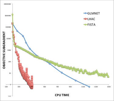
(a) GISETTE dense. (#Instances = 2000).

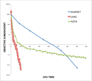
(b) RCV1 sparse. (#Instances = 2500).

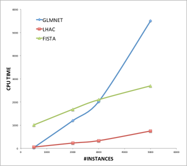
(c) GISETTE dense. #Instances from 500 to 5000.

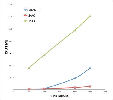
(d) RCV1 sparse. #Instances from 500 to 2500.

Figure 1: Convergence plots in 1(a) and 1(b) (the y-axes on log scale). Scalability plots in 1(c) and 1(d).

As can be seen from the results, the advantage of LHAC really lies in the fact that it absorbs the benefits from both the first order and the second order methods, such that it iterates fast, with low per iteration cost, and that it converges fast like other quasi-Newton methods, by taking advantage of the objective curvature information. For example, let us look at how FISTA compares with GLMNET in Table 1, which provides a good case to study the well-known trade-offs between first order and second order methods. Particularly, it can be seen that in most cases when $\epsilon$ is set to $10^{-2}$, FISTA takes up much less time to terminate than GLMNET. However, FISTA falls short when high precision is demanded, e.g., $\epsilon$ set to $10^{-5}$, in which case GLMNET almost always terminates faster than FISTA. Notably, LHAC is able to perform well in both cases. In fact, it is overwhelmingly faster than the other two in all but one experiment (the runtime difference between LHAC and GLMNET is close when the training size is sufficiently small), which brings us to another interesting aspect about LHAC. That is, the larger the size of the training set is, the larger the margin becomes between LHAC and GLMNET. We illustrate this observation in Figure 1(c) and 1(d), where the runtime of each algorithm ($\epsilon=10^{-5}$) is plotted against the training size. Note that the complexity of LHAC scales almost linearly with the problem size (with a much flatter rate than FISTA), while that of GLMNET increases nonlinearly. Figure 1(a) and 1(b) plot the change of objective subgradient against elapsed cputime in one experiment. Again, it can be observed that LHAC iterates as efficient as FISTA in the beginning, and while FISTA gradually slows down near the optimality, it continues to work as GLMNET until reaching the optimality tolerance $10^{-5}$.

Table 1: CPU time comparisons on real world classification data sets. Data set $rcv1$ has $47,326$ features and $0.17\%$ non-zeros; Data set $gisette$ has $5,000$ features and $99\%$ non-zeros. $rcv1_{500}$ denotes that the training set is $rcv1$ and $500$ training samples are used. $\epsilon$ indicates the optimization tolerance on the objective subgradient. The results show that LHAC is significantly faster than other methods.

Data set	$\epsilon$	cputime(in seconds)
		fista	glmnet	lhac
$rcv1_{500}$	$10^{-2}$	4.54	6.39	2.68
	$10^{-5}$	358.72	12.04	8.09
$rcv1_{1000}$	$10^{-2}$	14.28	6.18	3.53
	$10^{-5}$	572.41	18.13	14.13
$rcv1_{2000}$	$10^{-2}$	15.28	97.87	6.13
	$10^{-5}$	980.72	188.48	33.05
$rcv1_{2500}$	$10^{-2}$	17.71	170.13	9.95
	$10^{-5}$	1212.92	351.60	52.00
$gisette_{500}$	$10^{-2}$	52.91	10.93	3.23
	$10^{-5}$	1009.66	35.95	54.90
$gisette_{2000}$	$10^{-2}$	85.41	269.26	35.02
	$10^{-5}$	1686.69	1195.48	229.67
$gisette_{3000}$	$10^{-2}$	101.52	507.65	40.17
	$10^{-5}$	2241.95	2021.40	332.83
$gisette_{5000}$	$10^{-2}$	102.78	1758.98	112.11
	$10^{-5}$	2661.95	5935.72	752.87

4.2 Sparse Inverse Covariance Matrix Estimation

In this section we compare our algorithm LHAC with QUIC by Hsieh et al. (2011), a specialized solver that has been shown by Olsen et al. (2012) and Hsieh et al. (2011) to be the state of the art for sparse covariance selection problem defined below

$$\min_{X\succ 0}\quad f(X)=-\log\det X+\operatorname{tr}(SX)+\lambda||X||_{1}$$ (27)

where the optimization variables are in a matrix form $X\in\mathbb{R}^{p\times p}$ that is required to be positive definite.

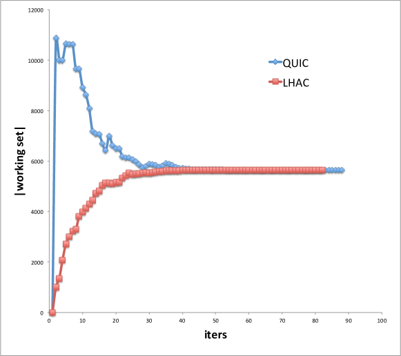
Figure 2: Comparing two strategies - the strategy used by QUIC and the one used by LHAC - of choosing the working set on ER data set. Note that the working set maintained by LHAC approaches the optimal size from below while that of QUIC from above.

For this experiment, we are interested in comparing the total complexity of the two algorithms. CPU time, as often used, will not be a reasonable complexity measure in this case, because QUIC is implemented in C++ and LHAC - in MATLAB. Instead, we decide to count the number of flops required by each algorithm to solve problem (27). Here we note that the work required by both algorithm consists mainly two parts – one for solving the subproblems and the other for computing Cholesky factorizations of $X$ during line search, and that the time either algorithm spends on the first part – solving the subproblems – generally takes around $95\sim 99\%$ of the total elapsed time, as observed in the experiments. Hence we focus our comparisons on the first part of the work – the one required by applying coordinate descent to solving subproblems, and we note that although LHAC generally requires more work in line search than QUIC (due to more outer iterations), it adds little to the total work for reasons stated above.

Table 2: Total complexity comparisons. $p$ stands for dimension. $\epsilon$ indicates the optimization tolerance on the objective subgradient.

Data set	$p$	$\epsilon$	Complexity($\times 10^{6}$)
			quic	lhac
Lymph	587	$10^{-2}$	47	13
		$10^{-6}$	105	45
ER	692	$10^{-2}$	218	78
		$10^{-6}$	353	217
Arabidopsis	834	$10^{-2}$	559	329
		$10^{-6}$	1001	804
Leukemia	1255	$10^{-2}$	2101	574
		$10^{-6}$	3028	1326
Hereditary	1869	$10^{-2}$	16558	8333
		$10^{-6}$	18519	16770

Now let us describe how we compute the total complexity. Let us use $\kappa_{o}$ to denote the number of outer iteration and $\kappa_{i}$ to denote the number of inner coordinate sweep. Let $T_{CD}$ stand for the number of flops one coordinate descent step takes. Then we define the total complexity by

$$Complexity=\kappa_{o}\kappa_{i}pT_{CD}$$ (28)

In theory, the two algorithms have similar $\kappa_{i}$ because they both apply coordinate descent to a lasso subproblem, but different $\kappa_{o}$ and $T_{CD}$. Particularly, $\kappa_{o}$ of QUIC is smaller than that of LHAC whereas $T_{CD}$ of LHAC is smaller than that of QUIC. The reason is that QUIC uses the actual Hessian matrix of the smooth part $\operatorname{tr}(SX)-\log\det X$ rather than the low-rank Hessian approximation as in LHAC, which results in a different convergence rate ($\kappa_{o}$) and also a different complexity ($T_{CD}$) in computing the coordinate descent step (24). As we discussed earlier, the special structure of the low-rank matrix enables LHAC to accelerate that step to $O(m)$ flops with $m$ a constant number (chosen as 10 for this experiment). Whereas in the case of QUIC, one coordinate step takes problem-dependent complexity $O(p)$ where $p$ is the dimension of $X$, but it achieves quadratic convergence when close to the optimality. The above observations make it interesting to see in practice how the $Complexity$, defined in (28), will compare for the two algorithms since it is not obvious which one is better through theoretical analysis alone.

The results are presented in Table 2, and in Figure 2 where we compare our active-set strategy with the one used by QUIC. The way we compute the $Complexity$ is by counting the number of flops in the coordinate descent step in each algorithm. For QUIC, we use their C++ implementation Hsieh et al. (2011) and add a counter directly in their code; for LHAC, we use our own MATLAB implementation. We report the results on real world data from gene expression networks preprocessed by Li and Toh (2010). We set the regularization parameter $\lambda=0.5$ for all the experiments as suggested in Li and Toh (2010). Similarly to the sparse logistic regression experiments, we solve each problem twice with different precision $\epsilon=10^{-2}$ and $\epsilon=10^{-6}$. Note that in all experiments QUIC consistently requires more flops to solve the problem than LHAC does. In one case where low precision is used it takes QUIC nearly three times more flops; even in the case QUIC is best at, where high precision is demanded, it can take QUIC 1.5 times more flops to achieve the same precision as LHAC did.

5 Conclusions

We have presented a general algorithm LHAC for efficiently using second-order information in training large-scale $\ell_{1}$-regularized convex models. We tested the algorithm on two instances of sparse logistic regression and five instances of sparse inverse covariance selection, and found that the algorithm is faster (sometimes overwhelmingly) than other specialized solvers on both models. The efficiency gains are due to two factors: the exploitation of the special structure present in the low-rank Hessian approximation matrix, and the greedy active-set strategy, which correctly identifies the non-zero features of the optimal solution.

References

- Andrew and Gao [2007] G. Andrew and J. Gao. Scalable training of l1-regularized log-linear models. ICML, pages 33–40, 2007.
- Beck and Teboulle [2009] A. Beck and M. Teboulle. A Fast Iterative Shrinkage-Thresholding Algorithm for Linear Inverse Problems. SIAM Journal on Imaging Sciences, 2(1):183–202, 2009.
- Bixby et al. [1992] R. E. Bixby, J. W. Gregory, I. J. Lustig, R. E. Marsten, and D. F. Shanno. Very large-scale linear programming: A case study in combining interior point and simplex methods. Operations Research, 40(5):pp. 885–897, 1992.
- Byrd et al. [2012] R. Byrd, G. Chin, J. Nocedal, and F. Oztoprak. A family of second-order methods for convex l1-regularized optimization. tech. rep., 2012.
- Donoho [1995] D. Donoho. De-noising by soft-thresholding. Information Theory, IEEE Transactions on, 41(3):613 –627, may 1995.
- Friedman et al. [2008] J. Friedman, T. Hastie, and R. Tibshirani. Sparse inverse covariance estimation with the graphical lasso. Biostatistics Oxford England, 9(3):432–41, 2008.
- Friedman et al. [2010] J. Friedman, T. Hastie, and R. Tibshirani. Regularization paths for generalized linear models via coordinate descent. Journal of Statistical Software, 33:1–22, 2010.
- Genkin et al. [2007] A. Genkin, D. D. Lewis, and D. Madigan. Large-scale bayesian logistic regression for text categorization. Technometrics, 49(3):291–304, 2007.
- Hsieh et al. [2011] C.-J. Hsieh, M. Sustik, I. Dhilon, and P. Ravikumar. Sparse inverse covariance matrix estimation using quadratic approximation. NIPS, 2011.
- Lewis et al. [2004] D. D. Lewis, Y. Yang, T. Rose, and F. Li. Rcv1: A new benchmark collection for text categorization research. JMLR, 5:361–397, 2004.
- Li and Toh [2010] L. Li and K.-C. Toh. An inexact interior point method for L1-regularized sparse covariance selection. Mathematical Programming, 2:291–315, 2010.
- Lin and Moré [1999] C.-J. Lin and J. Moré. Newtonʼs method for large bound-constrained optimization problems. SIAM Journal on Optimization, 9(4):1100, 1999.
- Nesterov [2007] Y. Nesterov. Gradient methods for minimizing composite objective function. CORE report, 2007.
- Nocedal and Wright [2006] J. Nocedal and S. J. Wright. Numerical Optimization. Springer Series in Operations Research. Springer, New York, NY, USA, 2nd edition, 2006.
- Olsen et al. [2012] P. A. Olsen, F. Oztoprak, J. Nocedal, and S. J. Rennie. Newton-Like Methods for Sparse Inverse Covariance Estimation, 2012.
- Scheinberg [2006] K. Scheinberg. An efficient implementation of an active set method for SVMs. JMLR, 7:2237–2257, 2006.
- Scheinberg and Rish [2009] K. Scheinberg and I. Rish. SINCO - a greedy coordinate ascent method for sparse inverse covariance selection problem. tech. rep., 2009.
- Scheinberg et al. [2010] K. Scheinberg, S. Ma, and D. Goldfarb. Sparse inverse covariance selection via alternating linearization methods. NIPS, 2010.
- Shalev-Shwartz and Tewari [2009] S. Shalev-Shwartz and A. Tewari. Stochastic methods for l1 regularized loss minimization. ICML, pages 929–936, 2009.
- Tibshirani [1996] R. Tibshirani. Regression shrinkage and selection via the lasso. Journal of the Royal Statistical Society Series B Methodological, 58(1):267–288, 1996.
- Tseng and Yun [2009] P. Tseng and S. Yun. A coordinate gradient descent method for nonsmooth separable minimization. Mathematical Programming, 117(1-2):387–423, Aug. 2009.
- Wright [2012] S. Wright. Accelerated block-coordinate relaxation for regularized optimization. SIAM Journal on Optimization, 22(1):159–186, 2012.
- Wright et al. [2009] S. J. Wright, R. D. Nowak, and M. A. T. Figueiredo. Sparse reconstruction by separable approximation. Trans. Sig. Proc., 57(7):2479–2493, July 2009.
- Yuan et al. [2010] G.-X. Yuan, K.-W. Chang, C.-J. Hsieh, and C.-J. Lin. A comparison of optimization methods and software for large-scale l1-regularized linear classification. JMLR, 11:3183–3234, 2010.
- Yuan et al. [2011] G.-X. Yuan, C.-H. Ho, and C.-J. Lin. An improved GLMNET for l1-regularized logistic regression and support vector machines. National Taiwan University, 2011.