Abstract

We address the problem of finding the maximizer of a nonlinear smooth function, that can only be evaluated point-wise, subject to constraints on the number of permitted function evaluations. This problem is also known as fixed-budget best arm identification in the multi-armed bandit literature. We introduce a Bayesian approach for this problem and show that it empirically outperforms both the existing frequentist counterpart and other Bayesian optimization methods. The Bayesian approach places emphasis on detailed modelling, including the modelling of correlations among the arms. As a result, it can perform well in situations where the number of arms is much larger than the number of allowed function evaluation, whereas the frequentist counterpart is inapplicable. This feature enables us to develop and deploy practical applications, such as automatic machine learning toolboxes. The paper presents comprehensive comparisons of the proposed approach, Thompson sampling, classical Bayesian optimization techniques, more recent Bayesian bandit approaches, and state-of-the-art best arm identification methods. This is the first comparison of many of these methods in the literature and allows us to examine the relative merits of their different features.

1 Introduction

We address the problem of finding the maximizer of a nonlinear smooth function $f:{\cal A}\mapsto\mathbb{R}$ which can only be evaluated point-wise. The function need not be convex, its derivatives may not be known, and the function evaluations will generally be corrupted by some form of noise. Importantly, we are interested in functions that are typically expensive to evaluate. Moreover, we will also assume a finite budget of $T$ function evaluations. This fixed-budget global optimization problem can be treated within the framework of sequential design. In this context, by allowing function queries $a_{t}\in\mathcal{A}$ to depend on previous points and their corresponding function evaluations, the algorithm must adaptively construct a sequence of queries (or actions) $a_{1:T}$ and afterwards return the element of highest expected value.

A typical example of this problem is that of automatic product testing (Kohavi et al., 2009; Scott, 2010), where common “products” correspond to configuration options for ads, websites, mobile applications, and online games. In this scenario, a company offers different product variations to a small subset of customers, with the goal of finding the most successful product for the entire customer base. The crucial problem is how best to query the smaller subset of users in order to find the best product with high probability. A second example, analyzed later in this paper, is that of automating machine learning. Here, the goal is to automatically select the best technique (boosting, random forests, support vector machines, neural networks, etc.) and its associated hyper-parameters for solving a machine learning task with a given dataset. For big datasets, cross-validation is very expensive and hence it is often important to find the best technique within a fixed budget of cross-validation tests (function evaluations).

In order to properly attack this problem there are three design aspects that must be considered. By taking advantage of correlation among different actions it is possible to learn more about a function than just its value at a specific query. This is particularly important when the number of actions greatly exceeds the finite query budget. In this same vein, it is important to take into account that a recommendation must be made at time $T$ in order to properly allocate actions and explore the space of possible optima. Finally, the fact that we are interested only in the value of the recommendation made at time $T$ should be handled explicitly. In other words, we are only interested in finding the best action and are concerned with the rewards obtained during learning only insofar as they inform us about this optimum.

In this work, we introduce a Bayesian approach that meets the above design goals and show that it empirically outperforms the existing frequentist counterpart (Gabillon et al., 2012). The Bayesian approach places emphasis on detailed modelling, including the modelling of correlations among the arms. As a result, it can perform well in situations where the number of arms is much larger than the number of allowed function evaluation, whereas the frequentist counterpart is inapplicable. The paper presents comprehensive comparisons of the proposed approach, Thompson sampling, classical Bayesian optimization techniques, more recent Bayesian bandit approaches, and state-of-the-art best arm identification methods. This is the first comparison of many of these methods in the literature and allows us to examine the relative merits of their different features. The paper also shows that one can easily obtain the same theoretical guarantees for the Bayesian approach that were previously derived in the frequentist setting (Gabillon et al., 2012).

2 Related work

Bayesian optimization has enjoyed success in a broad range of optimization tasks; see the work of Brochu et al. (2010b) for a broad overview. Recently, this approach has received a great deal of attention as a black-box technique for the optimization of hyperparameters (Snoek et al., 2012; Hutter et al., 2011; Wang et al., 2013b). This type of optimization combines prior knowledge about the objective function with previous observations to estimate the posterior distribution over $f$. The posterior distribution, in turn, is used to construct an acquisition function that determines what the next query point $a_{t}$ should be. Examples of acquisition functions include probability of improvement (PI), expected improvement (EI), Bayesian upper confidence bounds (UCB), and mixtures of these (Močkus, 1982; Jones, 2001; Srinivas et al., 2010; Hoffman et al., 2011). One of the key strengths underlying the use of Bayesian optimization is the ability to capture complicated correlation structures via the posterior distribution.

Many approaches to bandits and Bayesian optimization focus on online learning (e.g., minimizing cumulative regret) as opposed to optimization (Srinivas et al., 2010; Hoffman et al., 2011). In the realm of optimizing deterministic functions, a few works have proven exponential rates of convergence for simple regret (de Freitas et al., 2012; Munos, 2011). A stochastic variant of the work of Munos has been recently proposed by Valko et al. (2013); this approach takes a tree-based structure for expanding areas of the optimization problem in question, but it requires one to evaluate each cell many times before expanding, and so may prove expensive in terms of the number of function evaluations.

The problem of optimization under budget constraints has received relatively little attention in the Bayesian optimization literature, though some approaches without strong theoretical guarantees have been proposed recently (Azimi et al., 2011; Hennig and Schuler, 2012; Snoek et al., 2011; Villemonteix et al., 2009). In contrast, optimization under budget constraints has been studied in significant depth in the setting of multi-armed bandits (Bubeck et al., 2009; Audibert et al., 2010; Gabillon et al., 2011, 2012). Here, a decision maker must repeatedly choose query points, often discrete and known as “arms”, in order to observe their associated rewards (Cesa-Bianchi and Lugosi, 2006). However, unlike most methods in Bayesian optimization the underlying value of each action is generally assumed to be independent from all other actions. That is, the correlation structure of the arms is often ignored.

3 Problem formulation

In order to attack the problem of Bayesian optimization from a bandit perspective we will consider a discrete collection of arms $\mathcal{A}=\{1,\dots,K\}$ such that the immediate reward of pulling arm $k\in\mathcal{A}$ is characterized by a distribution $\nu_{k}$ with mean $\mu_{k}$. From the Bayesian optimization perspective we can think of this as a collection of points $\{a_{1},\dots,a_{K}\}$ where $\mu_{k}=f(a_{k})$. Note that while we will assume the distributions $\nu_{k}$ are independent of past actions this does not mean that the means of each arm cannot share some underlying structure—only that the act of pulling arm $k$ does not affect the future rewards of pulling this or any other arm. This distinction will be relevant later in this section.

The problem of identifying the best arm in this bandit problem can now be introduced as a sequential decision problem. At each round $t$ the decision maker will select or “pull” an arm $a_{t}\in\mathcal{A}$ and observe an independent sample $y_{t}$ drawn from the corresponding distribution $\nu_{a_{t}}$. At the beginning of each round $t$, the decision maker must decide which arm to select based only on previous interactions, which we will denote with the tuple $(a_{1:t-1},y_{1:t-1})$. For any arm $k$ we can also introduce the expected immediate regret of selecting that arm as

$$R_{k}=\mu^{*}-\mu_{k},$$ (1)

where $\mu^{*}$ denotes the expected value of the best arm. Note that while we are interested in finding the arm with the minimum regret, the exact value of this quantity is unknown to the learner.

In standard bandit problems the goal is generally to minimize the cumulative sum of immediate regrets incurred by the arm selection process. Instead, in this work we consider the pure exploration setting (Bubeck et al., 2009; Audibert et al., 2010), which divides the sampling process into two phases: exploration and evaluation. The exploration phase consists of $T$ rounds wherein a decision maker interacts with the bandit process by sampling arms. After these rounds, the decision maker must make a single arm recommendation $\Omega_{T}\in\mathcal{A}$. The performance of the decision maker is then judged only on the performance of this recommendation. The expected performance of this single recommendation is known as the simple regret, and we can write this quantity as $R_{\Omega_{T}}$. Given a tolerance $\epsilon>0$ we can also define the probability of error as the probability that $R_{\Omega_{T}}>\epsilon$. In this work, we will consider both the empirical probability that our regret exceeds some $\epsilon$ as well as the actual reward obtained.

4 Bayesian bandits

We will now consider a bandit problem wherein the distribution of rewards for each arm is assumed to depend on unknown parameters $\theta\in\Theta$ that are shared between all arms. We will write the reward distribution for arm $k$ as $\nu_{k}(\cdot|\theta)$. When considering the bandit problem from a Bayesian perspective, we will assume a prior density $\theta\sim\pi_{0}(\cdot)$ from which the parameters are drawn. Next, after $t-1$ rounds we can write the posterior density of these parameters as

$$\pi_{t}(\theta)\propto\pi_{0}(\theta)\prod_{n<t}\nu_{a_{n}}(y_{n}|\theta).$$ (2)

Here we can see the effect of choosing arm $a_{n}$ at each time $n$: we obtain information about $\theta$ only indirectly by way of the likelihood of these parameters given reward observations $y_{n}$. Note that this also generalizes the uncorrelated arms setting. If the rewards for each arm $k$ depend only on a parameter (or set of parameters) $\theta_{k}$, then at time $t$ the posterior for that parameter would only depend on those times in the past that we had pulled arm $k$.

We are, however, only partially interested in the posterior distribution of the parameters $\theta$. Instead, we are primarily concerned with the expected reward for each arm under these parameters, which can be written as $\mu_{k}=\mathbb{E}[Y|\theta]=\int y\,\nu_{k}(y|\theta)\,dy$. The true value of $\theta$ is unknown, but we have access to the posterior distribution $\pi_{t}(\theta)$. This distribution induces a marginal distribution over $\mu_{k}$, which we will write as $\rho_{kt}(\mu_{k})$. The distribution $\rho_{kt}(\mu_{k})$ can then be used to define upper and lower confidence bounds that hold with high probability and, hence, engineer acquisition functions that trade-off exploration and exploitation. We will derive an analytical expression for this distribution next.

We will assume that each arm $k$ is associated with a feature vector $x_{k}\in\mathbb{R}^{d}$ and where the rewards for pulling arm $k$ are normally distributed according to

$$\nu_{k}(y|\theta)=\mathcal{N}(y;x_{k}^{T}\theta,\sigma^{2})$$ (3)

with variance $\sigma^{2}$ and unknown $\theta\in\mathbb{R}^{d}$. The rewards for each arm are independent conditioned on $\theta$, but marginally dependent when this parameter is unknown. In particular the level of their dependence is given by the structure of the vectors $x_{k}$. By placing a prior $\theta\sim\mathcal{N}(0,\eta^{2}I)$ over the entire parameter vector we can compute a posterior distribution over this unknown quantity. One can also easily place an inverse-Gamma prior on $\sigma$ and compute the posterior analytically, but we will not describe this in order to keep the presentation simple.

The above linear observation model might seem restrictive. However, because we are only considering $K$ discrete actions (arms), it includes the Gaussian process (GP) setting. More precisely, let the matrix $G\in\mathbb{R}^{K\times K}$ be the covariance of a GP prior. Our experiments will detail two ways of constructing this covariance in practice. We can apply the following transformation to construct the design matrix $X=[x_{1}\dots x_{K}]^{T}$:

$$X=VD^{\frac{1}{2}},\ \text{where}\ G=VDV^{T}.$$

The rows of $X$ correspond to the vectors $x_{k}$ necessary for the construction of the observation model in Equation (3). By restricting ourselves to discrete actions spaces, we can also implement strategies such a Thompson sampling with GPs. The restriction to discrete action spaces poses some scaling challenges in high-dimensions, but it enables us to deploy a broad set of algorithms to attack low-dimensional problems. For this pragmatic reason, many existing popular Bayesian optimization software tools consider discrete actions only.

We will now let $X_{t}=[x_{a_{1}}\dots x_{a_{t-1}}]^{T}$ denote the design matrix and $Y_{t}=[y_{1}\dots y_{t-1}]^{T}$ the vector of observations at the beginning of round $t$. We can then write the posterior at time $t$ as $\pi_{t}(\theta)=\mathcal{N}(\theta;\hat{\theta}_{t},\hat{\Sigma}_{t})$, where

$$\hat{\Sigma}_{t}^{-1} =\sigma^{-2}X_{t}^{T}X_{t}+\eta^{-2}I,\text{ and}\quad$$ (4)

$$\hat{\theta}_{t} =\sigma^{-2}\hat{\Sigma}_{t}X_{t}^{T}Y_{t}.$$ (5)

From this formulation we can see that the expected reward associated with arm $k$ is marginally normal $\rho_{kt}(\mu_{k})=\mathcal{N}(\mu_{k};\hat{\mu}_{kt},\hat{\sigma}^{2}_{kt})$ with mean $\hat{\mu}_{kt}=x_{k}^{T}\hat{\theta}_{t}$ and variance $\hat{\sigma}_{kt}^{2}=x_{k}^{T}\hat{\Sigma}_{t}x_{k}$. Note also that the predictive distribution over rewards associated with the $k$th arm is normal as well, with mean $\hat{\mu}_{kt}$ and variance $\hat{\sigma}_{kt}^{2}+\sigma^{2}$. The previous derivations are textbook material; see for example Chapter 7 of (Murphy, 2012).

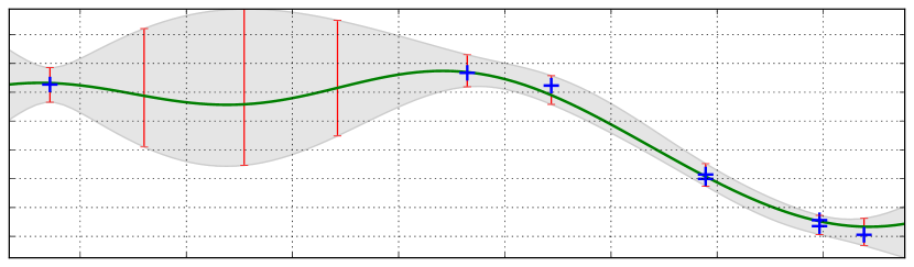
Figure 1: Example GP setting with discrete arms. The full GP is plotted with observations and confidence intervals at each of $K=10$ arms (mean and confidence intervals of $\rho_{kt}(\mu_{k})$). Shown in green is a single sample from the GP.

Figure 1 depicts an example of the mean and confidence intervals of $\rho_{kt}(\mu_{k})$, as well as a single random sample. Here the features $x_{k}$ were constructed by first forming the covariance matrix with an exponential kernel $k(x,x^{\prime})=\text{e}^{-(x-x^{\prime})^{2}}$ over the 1-dimensional discrete domain. As with standard Bayesian optimization with GPs, the statistics of $\rho_{kt}(\mu_{k})$ enable us to construct many different acquisition functions that trade-off exploration and exploitation. Thompson sampling in this setting also becomes straightforward, as we simply have to pick the maximum of the random sample from $\rho_{kt}(\mu_{k})$, at one of the discrete arms, as the next point to query.

5 Bayesian gap-based exploration

In this section we will introduce a gap-based solution to the Bayesian optimization problem, which we call BayesGap. This approach builds on the work of Gabillon et al. (2011, 2012), which we will refer to as UGap, and offers a principled way to incorporate correlation between different arms (whereas the earlier approach assumes all arms are independent).

At the beginning of round $t$ we will assume that the decision maker is equipped with high-probability upper and lower bounds $U_{k}(t)$ and $L_{k}(t)$ on the unknown mean $\mu_{k}$ for each arm. While this approach can encompass more general bounds, for the Gaussian-arms setting that we consider in this work we can define these quantities in terms of the mean and standard deviation, i.e. $\hat{\mu}_{kt}\pm\beta\hat{\sigma}_{kt}$. These bounds also give rise to a confidence diameter $s_{k}(t)=U_{k}(t)-L_{k}(t)=2\beta\hat{\sigma}_{kt}$.

Given bounds on the mean reward for each arm, we can then introduce the gap quantity

$$B_{k}(t)=\max_{i\neq k}U_{i}(t)-L_{k}(t),$$ (6)

which involves a comparison between the lower bound of arm $k$ and the highest upper bound among all alternative arms. Ultimately this quantity provides an upper bound on the simple regret (see Lemma B1 in the supplementary material) and will be used to define the exploration strategy. However, rather than directly finding the arm minimizing this gap, we will consider the two arms

$$J(t) =\operatorname*{arg\,min}_{k\in\mathcal{A}}B_{k}(t)\text{ and}$$

$$j(t) =\operatorname*{arg\,max}_{k\neq J(t)}U_{k}(t).$$

We will then define the exploration strategy as

$$a_{t} =\operatorname*{arg\,max}_{k\in\{j(t),J(t)\}}s_{k}(t).$$ (7)

Intuitively this strategy will select either the arm minimizing our bound on the simple regret (i.e. $J(t)$) or the best “runner up” arm. Between these two, the arm with the highest uncertainty will be selected, i.e. the one expected to give us the most information. Next, we will define the recommendation strategy as

$$\Omega_{T} =J\big{(}\operatorname*{arg\,min}_{t\leq T}B_{J(t)}(t)\big{)},$$ (8)

i.e. the proposal arm $J(t)$ which minimizes the regret bound, over all times $t\leq T$. The reason behind this particular choice is subtle, but is necessary for the proof of the method’s simple regret bound. In Algorithm 1 we show the pseudo-code for BayesGap.

Algorithm 1 BayesGap

1:  for $t=1,\dots,T$ do

2:     set $J(t)=\operatorname*{arg\,min}_{k\in\mathcal{A}}B_{k}(t)$

3:     set $j(t)=\operatorname*{arg\,min}_{k\neq J(t)}U_{k}(t)$

4:     select arm $a_{t}=\operatorname*{arg\,max}_{k\in\{j(t),J(t)\}}s_{k}(t)$

5:     observe $y_{t}\sim\nu_{a_{t}}(\cdot)$

6:     update posterior $\hat{\mu}_{kt}$ and $\hat{\sigma}_{kt}$

7:     update bound on $H_{\epsilon}$ and re-compute $\beta$

8:     update posterior bounds $U_{k}(t)$ and $L_{k}(t)$

9:  end for

10:  return  $\Omega_{T}=J\big{(}\operatorname*{arg\,min}_{t\leq T}B_{J(t)}(t)\big{)}$

We now turn to the problem of which value of $\beta$ to use. First, consider the quantity $\Delta_{k}=|\max_{i\neq k}\mu_{i}-\mu_{k}|$. For the best arm this coincides with a measure of the distance to the second-best arm, whereas for all other arms it is a measure of their sub-optimality. Given this quantity let $H_{k\epsilon}=\max(\tfrac{1}{2}(\Delta_{k}+\epsilon),\epsilon)$ be an arm-dependent hardness quantity; essentially our goal is to reduce the uncertainty in each arm to below this level, at which point with high probability we will identify the best arm. Now, given $H_{\epsilon}=\sum_{k}H_{k\epsilon}^{-2}$ we define our exploration constant as

$$\beta^{2}=\big{(}(T-K)/\sigma^{2}+\kappa/\eta^{2}\big{)}\big{/}(4H_{\epsilon})$$ (9)

where $\kappa=\sum_{k}\|x_{k}\|^{-2}$. We have chosen $\beta$ such that with high probability we recover an $\epsilon$-best arm, as detailed in the following theorem. This theorem relies on bounding the uncertainty for each arm by a function of the number of times that arm is pulled. Roughly speaking, if this bounding function is monotonically decreasing and if the bounds $U_{k}$ and $L_{k}$ hold with high probability we can then apply Theorem 2 to bound the simple regret of BayesGap.

Theorem 1.

Consider a $K$-armed Gaussian bandit problem, horizon $T$, and upper and lower bounds defined as above. For $\epsilon>0$ and $\beta$ defined as in Equation (9), the algorithm attains simple regret satisfying $\mathrm{Pr}(R_{\Omega_{T}}\leq\epsilon)\geq 1-KTe^{-\beta^{2}/2}$.

Proof.

Using the definition of the posterior variance for arm $k$, we can write the confidence diameter as

$$s_{k}(t) =2\beta\sqrt{x_{k}^{T}\hat{\Sigma}_{t}x_{k}}$$

$$=2\beta\sqrt{\sigma^{2}x_{k}^{T}\big{(}\textstyle\sum_{i}N_{i}(t-1)\,x_{i}x_{i}^{T}+\tfrac{\sigma^{2}}{\eta^{2}}I\big{)}^{-1}x_{k}}$$

$$\leq 2\beta\sqrt{\sigma^{2}x_{k}^{T}\big{(}N_{k}(t-1)\,x_{k}x_{k}^{T}+\tfrac{\sigma^{2}}{\eta^{2}}I\big{)}^{-1}x_{k}}.$$

In the second equality we decomposed the Gram matrix $X_{t}^{T}X_{t}$ in terms of a sum of outer products over the fixed vectors $x_{i}$. In the final inequality we noted that by removing samples we can only increase the variance term, i.e. here we have essentially replaced $N_{i}(t-1)$ with $0$ for $i\neq k$. We will let the result of this final inequality define an arm-dependent bound $g_{k}$. Letting $A=\tfrac{1}{N}\tfrac{\sigma^{2}}{\eta^{2}}$ we can simplify this quantity using the Sherman-Morrison formula as

$$g_{k}(N) =2\beta\sqrt{(\sigma^{2}/N)x_{k}^{T}\big{(}x_{k}x_{k}^{T}+AI\big{)}^{-1}x_{k}}$$

$$=2\beta\sqrt{\frac{\sigma^{2}}{N}\frac{\|x_{k}\|^{2}}{A}\Big{(}1-\frac{\|x_{k}\|^{2}/A}{1+\|x_{k}\|^{2}/A}\Big{)}}$$

$$=2\beta\sqrt{\frac{\sigma^{2}\|x_{k}\|^{2}}{\tfrac{\sigma^{2}}{\eta^{2}}+N\|x_{k}\|^{2}}},$$

which is monotonically decreasing in $N$. The inverse of this function can be solved for as

$$g^{-1}_{k}(s)=\frac{4(\beta\sigma)^{2}}{s^{2}}-\frac{\sigma^{2}}{\eta^{2}}\frac{1}{\|x_{k}\|^{2}}.$$

By setting $\sum_{k}g_{k}^{-1}(H_{k\epsilon})=T-K$ and solving for $\beta$ we then obtain the definition of this term given in the statement of the proposition. Finally, by reference to Lemma B4 (supplementary material) we can see that for each $k$ and $t$, the upper and lower bounds must hold with probability $1-e^{-\beta/2}$. These last two statements satisfy the assumptions of Theorem 2 (supplementary material), thus concluding our proof. ∎

Here we should note that while we are using Bayesian methodology to drive the exploration of the bandit, we are analyzing this using frequentist regret bounds. This is a common practice when analyzing the regret of Bayesian bandit methods (Srinivas et al., 2010; Kaufmann et al., 2012a). We should also point out that implicitly Theorem 2 assumes that each arm is pulled at least once regardless of its bound. However, in our setting we can avoid this in practice due to the correlation between arms.

One key thing to note is that the proof and derivation of $\beta$ given above explicitly require the hardness quantity $H_{\epsilon}$, which is unknown in most practical applications. Instead of requiring this quantity, our approach will be to adaptively estimate it. Intuitively, the quantity $\beta$ controls how much exploration BayesGap does (note that $\beta$ directly controls the width of the uncertainty $s_{k}(t)$). Further, $\beta$ is inversely proportional to $H_{\epsilon}$. As a result, in order to initially encourage more exploration we will lower bound the hardness quantity. In particular, we can do this by upper bounding each $\Delta_{k}$ by using conservative, posterior dependent upper and lower bounds on $\mu_{k}$. In this work we use three posterior standard deviations away from the posterior mean, i.e. $\hat{\mu}_{k}(t)\pm 3\hat{\sigma}_{kt}$. (We emphasize that these are not the same as $L_{k}(t)$ and $U_{k}(t)$.) Then the upper bound on $\Delta_{k}$ is simply

$$\hat{\Delta}_{k}=\max_{j\neq k}(\hat{\mu}_{j}+3\hat{\sigma}_{j})-(\hat{\mu}_{k}-3\hat{\sigma}_{k}).$$

From this point we can recompute $H_{\epsilon}$ and in turn recompute $\beta$ (step 7 in the pseudocode). For all experiments we will use this adaptive method.

Comparison with UGap. The method in this section provides a Bayesian version of the UGap algorithm which modifies the bounds used in this earlier algorithm’s arm selection step. By modifying step 6 of the BayesGap pseudo-code to use either Hoeffding or Bernstein bounds we can re-obtain the UGap algorithm. Note, however, that in doing so UGap assumes independent arms with bounded rewards.

We can now roughly compare UGap’s probability of error, i.e. $O(KT\exp(-\frac{T-K}{H_{\epsilon}}))$, with that of BayesGap, $O(KT\exp(-\frac{T-K+\kappa\sigma^{2}/\eta^{2}}{H_{\epsilon}\sigma^{2}}))$. We can see that with minor differences, these bounds are of the same order. First, we can ignore the additional $\sigma^{2}$ term as this quantity is primarily due to the distinction between bounded and Gaussian-distributed rewards. The $\eta^{2}$ term corresponds to the concentration of the prior, and we can see that the more concentrated the prior is (smaller $\eta$) the faster this rate is. Note, however, that the proof of BayesGap’s simple regret relies on the true rewards for each arm being within the support of the prior, so one cannot increase the algorithm’s performance by arbitrarily adjusting the prior. Finally, the $\kappa$ term is related to the linear relationship between different arms. Additional theoretical results on improving these bounds remains for future work.

6 Experiments

In the following subsections, we benchmark the proposed algorithm against a wide variety of methods on two real-data applications. In Section 6.1, we revisit the traffic sensor network problem of Srinivas et al. (2010). In Section 6.2, we consider the problem of automatic model selection and algorithm configuration.

6.1 Application to a traffic sensor network

In this experiment, we are given data taken from traffic speed sensors deployed along highway I-880 South in California. Traffic speeds were collected at $K=357$ sensor locations for all working days between 6AM and 11AM for an entire month. Our task is to identify the single location with the highest expected speed, i.e. the least congested. This data was also used in the work of Srinivas et al. (2010).

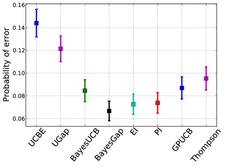
Figure 2: Probability of error on the optimization domain of traffic speed sensors. For this real data set, BayesGap provides considerable improvements over the Bayesian cumulative regret alternatives and the frequentist simple regret counterparts.

Naturally, the readings from different sensors are correlated, however, this correlation is not necessarily only due to geographical location. Therefore specifying a similarity kernel over the space of traffic sensor locations alone would be overly restrictive. Following the approach of Srinivas et al. (2010), we construct the design matrix treating two-thirds of the available data as historical and use the remaining third to evaluate the policies. In more detail, The GP kernel matrix $G\in\mathbb{R}^{K\times K}$ is set to be empirical covariance matrix of measurements for each of the $K$ sensor locations. As explained in Section 4, the corresponding design matrix is $X=VD^{\frac{1}{2}}$, where $G=VDV^{T}$.

Following Srinivas et al. (2010), we estimate the noise level $\sigma$ of the observation model using this data. We consider the average empirical variance of each individual sensor (i.e. the signal variance corresponding to the diagonal of $G$) and set the noise variance $\sigma^{2}$ to 5% of this value; this corresponds to $\sigma^{2}=4.78$. We choose a broad prior with regularization coefficient $\eta=20$.

In order to evaluate different bandit and Bayesian optimization algorithms, we use each of the remaining 840 sensor signals (the aforementioned third of the data) as the true mean vector $\mu$ for independent runs of the experiment. Note that using the model in this way enables us to evaluate the ground truth for each run (given by $\mu$, but not observed by the algorithm), and estimate the actual probability that the policies return the best arm.

In this experiment, as well as in the next one, we estimate the hardness parameter $H_{\epsilon}$ using the adaptive procedure outlined at the end of Section 5.

We benchmark the proposed algorithm (BayesGap) against the following methods:

(1) UCBE: Introduced by Audibert et al. (2010); this is a variant of the classical UCB policy of Auer et al. (2002) that replaces the $\log(t)$ exploration term of UCB with a constant of order $\log(T)$ for known horizon $T$.

(2) UGap: A gap-based exploration approach introduced by Gabillon et al. (2012).

(3) BayesUCB and GPUCB: Bayesian extensions of UCB which derive their confidence bounds from the posterior. Introduced by Kaufmann et al. (2012a) and Srinivas et al. (2010) respectively.

(4) Thompson sampling: A randomized, Bayesian index strategy wherein the $k$th arm is selected with probability given by a single-sample Monte Carlo approximation to the posterior probability that the arm is the maximizer (Chapelle and Li, 2012; Kaufmann et al., 2012b; Agrawal and Goyal, 2013).

(5) Probability of Improvement (PI): A classic Bayesian optimization method which selects points based on their probability of improving upon the current incumbent.

(6) Expected Improvement (EI): A Bayesian optimization, related to PI, which selects points based on the expected value of their improvement.

Note that techniques (1) and (2) above attack the problem of best arm identification and use bounds which encourage more aggressive exploration. However, they do not take correlation into account. On the other hand, techniques such ad (3) are designed for cumulative regret, but model the correlation among the arms. It might seem at first that we are comparing apples and oranges. However, the purpose of comparing these methods, even if their objectives are different, is to understand empirically what aspects of these algorithms matter the most in practical applications.

The results, shown in Figure 2, are the probabilities of error for each strategy, using a time horizon of $T=400$. (Here we used $\epsilon=0$, but varying this quantity had little effect on the performance of each algorithm.) By looking at the results, we quickly learn that techniques that model correlation perform better than the techniques designed for best arm identification, even when they are being evaluated in a best arm identification task. The important conclusion is that one must always invest effort in modelling the correlation among the arms.

The results also show that BayesGap does better than alternatives in this domain. This is not surprising because BayesGap is the only competitor that addresses budgets, best arm identification and correlation simultaneously.

6.2 Automatic machine learning

There exist many machine learning toolboxes, such as Weka and scikit-learn. However, for a great many data practitioners interested in finding the best technique for a predictive task, it is often hard to understand what each technique in the toolbox does. Moreover, each technique can have many free hyper-parameters that are not intuitive to most users.

Bayesian optimization techniques have already been proposed to automate machine learning approaches, such as MCMC inference (Mahendran et al., 2012; Hamze et al., 2013; Wang et al., 2013a), deep learning (Bergstra et al., 2011), preference learning (Brochu et al., 2007, 2010a), reinforcement learning and control (Martinez-Cantin et al., 2007; Lizotte et al., 2012), and more (Snoek et al., 2012). In fact, methods to automate entire toolboxes (Weka) have appeared very recently (Thornton et al., 2013), and go back to old proposals for classifier selection (Maron and Moore, 1994).

Here, we will demonstrate BayesGap by automating regression with scikit-learn. Our focus will be on minimizing the cost of cross-validation in the domain of big data. In this setting, training and testing each model can take a prohibitive long time. If we are working under a finite budget, say if we only have three days before a conference deadline or the deployment of a product, we cannot afford to try all models in all cross-validation tests. However, it is possible to use techniques such as BayesGap and Thompson sampling to find the best model with high probability. In our setting, the action of “pulling an arm” will involve selecting a model, splitting the dataset randomly into training and test sets, training the model, and recording the test-set performance.

In this bandit domain, our arms will consist of five scikit-learn techniques and associated parameters selected on a discrete grid. We consider the following methods for regression: Lasso (8 models) with regularization parameters alpha = (0.0001, 0.0005, 0.001, 0.005, 0.01, 0.05, 0.1, 0.5), Random Forests (64 models) where we vary the number of trees, n_estimators=(1,10,100,1000), the minimum number of training examples in a node to split min_samples_split=(1,3,5,7) and the minimum number of training examples in a leaf min_samples_leaf=(2,6,10,14), linSVM (16 models) where we vary the penalty parameter C= (0.001, 0.01, 0.1, 1) and the tolerance parameter epsilon=(0.0001, 0.001, 0.01, 0.1), rbfSVM (64 models) where we use the same grid as above for C and epsilon, and we add a third parameter which is the length scale $\gamma$ of the RBF kernel used by the SVM $\text{{gamma}}=(0.025,0.05,0.1,0.2)$, and K-nearest neighbors (8 models) where we vary number of neighbors $\text{{n\_neighbors}}=(1,3,5,7,9,11,13,15).$ The total number of models is 160. Within a class of regressors, we model correlation using a squared exponential kernel with unit length scale, i.e., $k(x,x^{\prime})=\text{e}^{-(x-x^{\prime})^{2}}$. Using this kernel, we compute a kernel matrix $G$ and construct the design matrix as before.

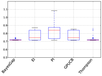
Figure 3: Boxplot of RMSE over 100 runs with a fixed budget of $T=10$. EI, PI, and GPUCB get stuck in local minima. Note: lower is better.

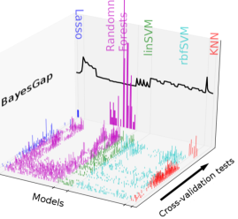
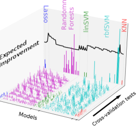
Figure 4: Allocations and recommendations of BayesGap (top) and EI (bottom) over 100 runs at a budget of $T=40$ training and validation tests, and for 160 models (i.e., more arms than possible observations). Histograms along the floor of the plot show the arms pulled at each round while the histogram on the far wall shows the final arm recommendation over 100 different runs. The solid black line on the far wall shows the estimated “ground truth” RMSE for each model. Note that EI quite often gets stuck in a locally optimal rbfSVM.

When an arm is pulled we select training and test sets that are each 10% of the size of the original, and ignore the remaining 80% for this particular arm pull. We then train the selected model on the training set, and test on the test set. This specific form of cross-validation is similar to that of repeated learning-testing (Arlot and Celisse, 2010; Burman, 1989).

We use the wine dataset from the UCI Machine Learning Repository, where the task is to predict the quality score (between 0 and 10) of a wine given 11 attributes of its chemistry. We repeat the experiment 100 times. We report, for each method, an estimate of the RMSE for the recommended models on each run. Unlike in the previous section, we do not have the ground truth generalization error, and in this scenario it is difficult to estimate the actual “probability of error”. Instead we report the RMSE, but remark that this is only a proxy for the error rate that we are interested in.

The performance of the final recommendations for each strategy and a fixed budget of $T=10$ tests is shown in Figure 3. The results for other budgets are almost identical. It must be emphasized that the number of allowed function evaluations (10 tests) is much smaller than the number of arms (160 models). Hence, frequentist approaches that require pulling all arms, e.g. UGap, are inapplicable in this domain.

The results indicate that Thompson and BayesGap are the best choices for this domain. Figure 4 shows the individual arms pulled and recommended by BayesGap (above) and EI (bottom), over each of the 100 runs, as well as an estimate of the ground truth RMSE for each individual model. EI and PI often get trapped in local minima. Due to the randomization inherent to Thompson sampling, it explores more, but in a more uniform manner (possibly explaining its poor results in the previous experiment).

7 Conclusion

We proposed a Bayesian optimization method for best arm identification with a fixed budget. The method involves modelling of the correlation structure of the arms via Gaussian process kernels. As a result of combining all these elements, the proposed method outperformed techniques that do not model correlation or that are designed for different objectives (typically cumulative regret). This strategy opens up room for greater automation in practical domains with budget constraints, such as the automatic machine learning application described in this paper.

Although we focused on a Bayesian treatment of the UGap algorithm, the same approach could conceivably be applied to other techniques such as UCBE. As demonstrated by Srinivas et al. (2010) and in this paper, it is possible to easily show that the Bayesian bandits obtain similar bounds as the frequentist methods. However, in our case, we conjecture that much stronger bounds should be possible if we consider all the information brought in by the priors and measurement models.

Appendix A Theorem 2

The proof of this section and the lemmas of the next section follow from the proofs of Gabillon et al. (2012). The modifications we have made to this proof correspond to the introduction of the function $g_{k}$ which bounds the uncertainty $s_{k}$ in order to make it simpler to introduce other models. We also introduce a sufficient condition on this bound, i.e. that it is monotonically decreasing in $N$ in order to bound the arm pulls with respect to $g_{k}^{-1}$. Ultimately, this form of the theorem reduces the problem of of proving a regret bound to that of checking a few properties of the uncertainty model.

Theorem 2.

Consider a bandit problem with horizon $T$ and $K$ arms. Let $U_{k}(t)$ and $L_{k}(t)$ be upper and lower bounds that hold for all times $t\leq T$ and all arms $k\leq K$ with probability $1-\delta$. Finally, let $g_{k}$ be a monotonically decreasing function such that $s_{k}(t)\leq g_{k}(N_{k}(t-1))$ and $\sum_{k}g_{k}^{-1}(H_{k\epsilon})\leq T-K$. We can then bound the simple regret as

$$\mathrm{Pr}(R_{\Omega_{T}}\leq\epsilon)\geq 1-KT\delta.$$ (10)

Proof.

We will first define the event $\mathcal{E}$ such that on this event every mean is bounded by its associated bounds for all times $t$. More precisely we can write this as

$$\mathcal{E}=\{\forall k\leq K,\forall t\leq T,L_{k}(t)\leq\mu_{k}\leq U_{k}(t)\}.$$

By definition, these bounds are given such that the probability of deviating from a single bound is $\delta$. Using a union bound we can then bound the probability of remaining within all bounds as $\mathrm{Pr}(\mathcal{E})\geq 1-KT\delta$.

We will next condition on the event $\mathcal{E}$ and assume regret of the form $R_{\Omega_{T}}>\epsilon$ in order to reach a contradiction. Upon reaching said contradiction we can then see that the simple regret must be bounded by $\epsilon$ with probability given by the probability of event $\mathcal{E}$, as stated above. As a result we need only show that a contradiction occurs.

We will now define $\tau=\operatorname*{arg\,min}_{t\leq T}B_{J(t)}(t)$ as the time at which the recommended arm attains the minimum bound, i.e. $\Omega_{T}=J(\tau)$ as defined in (8). Let $t_{k}\leq T$ be the last time at which arm $k$ is pulled. Note that each arm must be pulled at least once due to the initialization phase. We can then show the following sequence of inequalities:

$$\min(0,s_{k}(t_{k})-\Delta_{k})+s_{k}(t_{k}) \geq B_{J(t_{k})}(t_{k})$$ (a)

$$\geq B_{\Omega_{T}}(\tau)$$ (b)

$$\geq R_{\Omega_{T}}$$ (c)

$$>\epsilon.$$ (d)

Of these inequalities, (a) holds by Lemma B3, (c) holds by Lemma B1, and (d) holds by our assumption on the simple regret. The inequality (b) holds due to the definition $\Omega_{T}$ and time $\tau$. Note, that we can also write the preceding inequality as two cases

$$s_{k}(t_{k})>2s_{k}(t_{k})-\Delta_{k}>\epsilon, \quad\text{if }\Delta_{k}>s_{k}(t_{k});$$

$$2s_{k}(t_{k})-\Delta_{k}\geq s_{k}(t_{k})>\epsilon, \quad\text{if }\Delta_{k}\leq s_{k}(t_{k})$$

This leads to the following bound on the confidence diameter,

$$s_{k}(t_{k})>\max(\tfrac{1}{2}(\Delta_{k}+\epsilon),\epsilon)=H_{k\epsilon}$$

which can be obtained by a simple manipulation of the above equations. More precisely we can notice that in each case, $s_{k}(t_{k})$ upper bounds both $\epsilon$ and $\tfrac{1}{2}(\Delta_{k}+\epsilon)$, and thus it obviously bounds their maximum.

Now, for any arm $k$ we can consider the final number of arm pulls, which we can write as

$$N_{k}(T)=N_{k}(t_{k}-1)+1 \leq g^{-1}(s_{k}(t_{k}))+1$$

$$<g^{-1}(H_{k\epsilon})+1.$$

This holds due to the definition of $g$ as a monotonic decreasing function, and the fact that we pull each arm at least once during the initialization stage. Finally, by summing both sides with respect to $k$ we can see that $\sum_{k}g^{-1}(H_{k\epsilon})+K>T$, which contradicts our definition of $g$ in the Theorem statement. ∎

Appendix B Lemmas

In order to simplify notation in this section, we will first introduce $B(t)=\min_{k}B_{k}(t)$ as the minimizer over all gap indices for any time $t$. We will also note that this term can be rewritten as

$$B(t)=B_{J(t)}(t)=U_{j(t)}(t)-L_{J(t)}(t),$$

which holds due to the definitions of $j(t)$ and $J(t)$.

Lemma B1.

For any sub-optimal arm $k\neq k^{*}$, any time $t\in\{1,\dots,T\}$, and on event $\mathcal{E}$, the immediate regret of pulling that arm is upper bounded by the index quantity, i.e. $B_{k}(t)\geq R_{k}$.

Proof.

We can start from the definition of the bound and expand this term as

$$B_{k}(t) =\max_{i\neq k}U_{i}(t)-L_{k}(t)$$

$$\geq\max_{i\neq k}\mu_{i}-\mu_{k}=\mu^{*}-\mu_{k}=R_{k}.$$

The first inequality holds due to the assumption of event $\mathcal{E}$, whereas the following equality holds since we are only considering sub-optimal arms, for which the best alternative arm is obviously the optimal arm. ∎

Lemma B2.

For any time $t$ let $k=a_{t}$ be the arm pulled, for which the following statements hold:

$$\textrm{if }k=j(t),\textrm{ then }L_{j(t)}(t)\leq L_{J(t)}(t),$$

$$\textrm{if }k=J(t),\textrm{ then }U_{j(t)}(t)\leq U_{J(t)}(t).$$

Proof.

We can divide this proof into two cases based on which of the two arms is selected.

Case 1: let $k=j(t)$ be the arm selected. We will then assume that $L_{j(t)}(t)>L_{J(t)}(t)$ and show that this is a contradiction. By definition of the arm selection rule we know that $s_{j(t)}(t)\geq s_{J(t)}(t)$, from which we can easily deduce that $U_{j(t)}(t)>U_{J(t)}(t)$ by way of our first assumption. As a result we can see that

$$B_{j(t)}(t) =\max_{j\neq j(t)}U_{j}(t)-L_{j(t)}(t)$$

$$<\max_{j\neq J(t)}U_{j}(t)-L_{J(t)}(t)=B_{J(t)}(t).$$

This inequality holds due to the fact that arm $j(t)$ must necessarily have the highest upper bound over all arms. However, this contradicts the definition of $J(t)$ and as a result it must hold that $L_{j(t)}(t)\leq L_{J(t)}(t)$.

Case 2: let $k=J(t)$ be the arm selected. The proof follows the same format as that used for $k=j(t)$. ∎

Corollary B2.

If arm $k=a_{t}$ is pulled at time $t$, then the minimum index is bounded above by the uncertainty of arm $k$, or more precisely

$$B(t)\leq s_{k}(t).$$

Proof.

We know that $k$ must be restricted to the set $\{j(t),J(t)\}$ by definition. We can then consider the case that $k=j(t)$, and by Lemma B2 we know that this imposes an order on the lower bounds of each possible arm, allowing us to write

$$B(t)\leq U_{j(t)}(t)-L_{j(t)}(t)=s_{j(t)}(t)$$

from which our corollary holds. We can then easily see that a similar argument holds for $k=J(t)$ by ordering the upper bounds, again via Lemma B2. ∎

Lemma B3.

On event $\mathcal{E}$, for any time $t\in\{1,\dots,T\}$, and for arm $k=a_{t}$ the following bound holds on the minimal gap,

$$B(t)\leq\min(0,s_{k}(t)-\Delta_{k})+s_{k}(t).$$

Proof.

In order to prove this lemma we will consider a number of cases based on which of $k\in\{j(t),J(t)\}$ is selected and whether or not one or neither of these arms corresponds to the optimal arm $k^{*}$. Ultimately, this results in six cases, the first three of which we will present are based on selecting arm $k=j(t)$.

Case 1: consider $k^{*}=k=j(t)$. We can then see that the following sequence of inequalities holds,

$$\mu_{(2)}\stackrel{{\scriptstyle(a)}}{{\geq}}\mu_{J(t)}(t)\stackrel{{\scriptstyle(b)}}{{\geq}}L_{J(t)}(t)\stackrel{{\scriptstyle(c)}}{{\geq}}L_{j(t)}(t)\stackrel{{\scriptstyle(d)}}{{\geq}}\mu_{k}-s_{k}(t).$$

Here (b) and (d) follow directly from event $\mathcal{E}$ and (c) follows from Lemma B2. Inequality (a) follows trivially from our assumption that $k=k^{*}$, as a result $J(t)$ can only be as good as the 2nd-best arm. Using the definition of $\Delta_{k}$ and the fact that $k=k^{*}$, the above inequality yields

$$s_{k}(t)-(\mu_{k}-\mu_{(2)})=s_{k}(t)-\Delta_{k}\geq 0$$

Therefore the $\min$ in the result of Lemma B3 vanishes and the result follows from Corollary B2.

Case 2: consider $k=j(t)$ and $k^{*}=J(t)$. We can then write

$$B(t) =U_{j(t)}(t)-L_{J(t)}(t)$$

$$\leq\mu_{j(t)}(t)+s_{j(t)}(t)-\mu_{J(t)}(t)+s_{J(t)}(t)$$

$$\leq\mu_{k}-\mu^{*}+2s_{k}(t)$$

where the first inequality holds from event $$\mathcal{E}$$, and the second holds because by definition the selected arm must have higher uncertainty. We can then simplify this as

$$=2s_{k}(t)-\Delta_{k}$$

$$\leq\min(0,s_{k}(t)-\Delta_{k})+s_{k}(t),$$

where the last step evokes Corollary B2.

Case 3: consider $k=j(t)\neq k^{*}$ and $J(t)\neq k^{*}$. We can then write the following sequence of inequalities,

$$\mu_{j(t)}(t)+s_{j(t)}(t)\stackrel{{\scriptstyle(a)}}{{\geq}}U_{j(t)}(t)\stackrel{{\scriptstyle(b)}}{{\geq}}U_{k^{*}}(t)\stackrel{{\scriptstyle(c)}}{{\geq}}\mu^{*}.$$

Here (a) and (c) hold due to event $\mathcal{E}$ and (b) holds since by definition $j(t)$ has the highest upper bound other than $J(t)$, which in turn is not the optimal arm by assumption in this case. By simplifying this expression we obtain $s_{k}(t)-\Delta_{k}\geq 0$, and hence the result follows from Corollary B2 as in Case 1.

Cases 4–6: consider $k=J(t)$. The proofs for these three cases follow the same general form as the above cases and is omitted. Cases 1 through 6 cover all possible scenarios and prove Lemma B3. ∎

Lemma B4.

Consider a normally distributed random variable $X\sim\mathcal{N}(\mu,\sigma^{2})$ and $\beta\geq 0$. The probability that $X$ is within a radius of $\beta\sigma$ from its mean can then be written as

$$\mathrm{Pr}\big{(}|X-\mu|\leq\beta\sigma\big{)}\geq 1-e^{-\beta^{2}/2}.$$

Proof.

Consider $Z\sim\mathcal{N}(0,1)$. The probability that $Z$ exceeds some positive bound $c>0$ can be written

$$\mathrm{Pr}(Z>c) =\frac{e^{-c^{2}/2}}{\sqrt{2\pi}}\int_{c}^{\infty}e^{(c^{2}-z^{2})/2}\,dz$$

$$=\frac{e^{-c^{2}/2}}{\sqrt{2\pi}}\int_{c}^{\infty}e^{-(z-c)^{2}/2-c(z-c)}\,dz$$

$$\leq\frac{e^{-c^{2}/2}}{\sqrt{2\pi}}\int_{c}^{\infty}e^{-(z-c)^{2}/2}\,dz=\tfrac{1}{2}e^{-c^{2}/2}.$$

The inequality holds due to the fact that $e^{-c(z-c)}\leq 1$ for $z\geq c$. Using a union bound we can then bound both sides as $\mathrm{Pr}(|Z|>c)\leq e^{-c^{2}/2}$. Finally, by setting $Z=(X-\mu)/\sigma$ and $c=\beta$ we obtain the bound stated above. ∎

References

- Agrawal and Goyal [2013] S. Agrawal and N. Goyal. Thompson sampling for contextual bandits with linear payoffs. In ICML, 2013.
- Arlot and Celisse [2010] S. Arlot and A. Celisse. A survey of cross-validation procedures for model selection. Statistics Surveys, 4:40–79, 2010.
- Audibert et al. [2010] J.-Y. Audibert, S. Bubeck, and R. Munos. Best arm identification in multi-armed bandits. In Conference on Learning Theory, 2010.
- Auer et al. [2002] P. Auer, N. Cesa-Bianchi, and P. Fischer. Finite-time analysis of the multiarmed bandit problem. Machine Learning, 47(2):235–256, 2002.
- Azimi et al. [2011] J. Azimi, A. Fern, and X. Fern. Budgeted optimization with concurrent stochastic-duration experiments. In NIPS, pages 1098–1106, 2011.
- Bergstra et al. [2011] J. Bergstra, R. Bardenet, Y. Bengio, and B. Kégl. Algorithms for hyper-parameter optimization. In NIPS, pages 2546–2554, 2011.
- Brochu et al. [2007] E. Brochu, N. de Freitas, and A. Ghosh. Active preference learning with discrete choice data. In NIPS, pages 409–416, 2007.
- Brochu et al. [2010a] E. Brochu, T. Brochu, and N. de Freitas. A Bayesian interactive optimization approach to procedural animation design. In ACM SIGGRAPH/Eurographics Symposium on Computer Animation, pages 103–112, 2010a.
- Brochu et al. [2010b] E. Brochu, V. Cora, and N. de Freitas. A tutorial on Bayesian optimization of expensive cost functions. Technical Report arXiv:1012.2599, arXiv, 2010b.
- Bubeck et al. [2009] S. Bubeck, R. Munos, and G. Stoltz. Pure exploration in multi-armed bandits problems. In International Conference on Algorithmic Learning Theory, 2009.
- Burman [1989] P. Burman. A comparative study of ordinary cross-validation, v-fold cross-validation and the repeated learning-testing methods. Biometrika, 76(3):pp. 503–514, 1989.
- Cesa-Bianchi and Lugosi [2006] N. Cesa-Bianchi and G. Lugosi. Prediction, Learning, and Games. Cambridge University Press, New York, 2006.
- Chapelle and Li [2012] O. Chapelle and L. Li. An empirical evaluation of Thompson sampling. In NIPS, 2012.
- de Freitas et al. [2012] N. de Freitas, A. Smola, and M. Zoghi. Exponential Regret Bounds for Gaussian Process Bandits with Deterministic Observations. In ICML, 2012.
- Gabillon et al. [2011] V. Gabillon, M. Ghavamzadeh, A. Lazaric, and S. Bubeck. Multi-bandit best arm identification. In NIPS, 2011.
- Gabillon et al. [2012] V. Gabillon, M. Ghavamzadeh, and A. Lazaric. Best arm identification: A unified approach to fixed budget and fixed confidence. In NIPS, 2012.
- Hamze et al. [2013] F. Hamze, Z. Wang, and N. de Freitas. Self-avoiding random dynamics on integer complex systems. ACM Transactions on Modelling and Computer Simulation, 23(1):9:1–9:25, 2013.
- Hennig and Schuler [2012] P. Hennig and C. Schuler. Entropy search for information-efficient global optimization. JMLR, 13:1809–1837, 2012.
- Hoffman et al. [2011] M. W. Hoffman, E. Brochu, and N. de Freitas. Portfolio allocation for Bayesian optimization. In UAI, pages 327–336, 2011.
- Hutter et al. [2011] F. Hutter, H. H. Hoos, and K. Leyton-Brown. Sequential model-based optimization for general algorithm configuration. In Proceedings of LION-5, page 507 523, 2011.
- Jones [2001] D. Jones. A taxonomy of global optimization methods based on response surfaces. J. of Global Optimization, 21(4):345–383, 2001.
- Kaufmann et al. [2012a] E. Kaufmann, O. Cappé, and A. Garivier. On Bayesian upper confidence bounds for bandit problems. In AIStats, 2012a.
- Kaufmann et al. [2012b] E. Kaufmann, N. Korda, and R. Munos. Thompson sampling: an asymptotically optimal finite-time analysis. In International Conference on Algorithmic Learning Theory, 2012b.
- Kohavi et al. [2009] R. Kohavi, R. Longbotham, D. Sommerfield, and R. Henne. Controlled experiments on the web: survey and practical guide. Data Mining and Knowledge Discovery, 18:140–181, 2009.
- Lizotte et al. [2012] D. J. Lizotte, R. Greiner, and D. Schuurmans. An experimental methodology for response surface optimization methods. Journal of Global Optimization, 53(4):699–736, 2012.
- Mahendran et al. [2012] N. Mahendran, Z. Wang, F. Hamze, and N. de Freitas. Adaptive MCMC with Bayesian optimization. Journal of Machine Learning Research - Proceedings Track, 22:751–760, 2012.
- Maron and Moore [1994] O. Maron and A. W. Moore. Hoeffding races: Accelerating model selection search for classification and function approximation. In NIPS, pages 59–66, 1994.
- Martinez-Cantin et al. [2007] R. Martinez-Cantin, N. de Freitas, A. Doucet, and J. A. Castellanos. Active policy learning for robot planning and exploration under uncertainty. 2007.
- Močkus [1982] J. Močkus. The Bayesian approach to global optimization. In Systems Modeling and Optimization, volume 38, pages 473–481. Springer, 1982.
- Munos [2011] R. Munos. Optimistic optimization of a deterministic function without the knowledge of its smoothness. In NIPS, pages 783–791, 2011.
- Murphy [2012] K. P. Murphy. Machine learning: A probabilistic perspective. Cambridge, MA, 2012.
- Scott [2010] S. Scott. A modern Bayesian look at the multi-armed bandit. Applied Stochastic Models in Business and Industry, 26(6), 2010.
- Snoek et al. [2011] J. Snoek, H. Larochelle, and R. P. Adams. Opportunity cost in Bayesian optimization. In Neural Information Processing Systems Workshop on Bayesian Optimization, 2011.
- Snoek et al. [2012] J. Snoek, H. Larochelle, and R. Adams. Practical Bayesian optimization of machine learning algorithms. In NIPS, pages 2960–2968, 2012.
- Srinivas et al. [2010] N. Srinivas, A. Krause, S. M. Kakade, and M. Seeger. Gaussian process optimization in the bandit setting: No regret and experimental design. In ICML, pages 1015–1022, 2010.
- Thornton et al. [2013] C. Thornton, F. Hutter, H. H. Hoos, and K. Leyton-Brown. Auto-WEKA: Combined selection and hyperparameter optimization of classification algorithms. In KDD, pages 847–855, 2013.
- Valko et al. [2013] M. Valko, A. Carpentier, and R. Munos. Stochastic simultaneous optimistic optimization. In ICML, 2013.
- Villemonteix et al. [2009] J. Villemonteix, E. Vazquez, and E. Walter. An informational approach to the global optimization of expensive-to-evaluate functions. Journal of Global Optimization, 44(4):509–534, 2009.
- Wang et al. [2013a] Z. Wang, S. Mohamed, and N. de Freitas. Adaptive Hamiltonian and Riemann manifold Monte Carlo samplers. In ICML, 2013a.
- Wang et al. [2013b] Z. Wang, M. Zoghi, D. Matheson, F. Hutter, and N. de Freitas. Bayesian optimization in high dimensions via random embeddings. In IJCAI, 2013b.