The spectra of jet bases in FR I radio galaxies: implications for particle acceleration

Abstract

We present accurate, spatially resolved imaging of radio spectra at the bases of jets in eleven low-luminosity (Fanaroff-Riley I) radio galaxies, derived from Very Large Array (VLA) observations. We pay careful attention to calibration and to the effects of random and systematic errors, and we base the flux-density scale on recent measurements of VLA primary amplitude calibrators by Perley & Butler (2013). We show images and profiles of spectral index over the frequency range 1.4 – 8.5 GHz, together with values integrated over fiducial regions defined by our relativistic models of the jets. We find that the spectral index $\alpha$, defined in the sense $I(\nu)\propto\nu^{-\alpha}$, decreases with distance from the nucleus in all of the jets. The mean spectral indices are $0.66\pm 0.01$ where the jets first brighten abruptly and $0.59\pm 0.01$ after they recollimate. The mean change in spectral index between these locations, which is independent of calibration and flux-density scale errors and is therefore more accurately and robustly measured, is $-0.067\pm 0.006$. Our jet models associate the decrease in spectral index with a bulk deceleration of the flow from $\approx 0.8c$ to $\la 0.5c$. We suggest that the decrease is the result of a change in the characteristics of ongoing particle acceleration. One possible acceleration mechanism is the first-order Fermi process in mildly relativistic shocks: in the Bohm limit, the index of the electron energy spectrum, $p=2\alpha+1$, is slightly larger than 2 and decreases with velocity upstream of the shock. This possibility is consistent with our measurements, but requires shocks throughout the jet volume rather than at a few discrete locations. A second possibility is that two acceleration mechanisms operate in these jets: one (with $p=2.32$) dominant close to the galactic nucleus and associated with high flow speeds, another (with $p=2.18$) taking over at larger distances and slower flow speeds.

1 Introduction

Jets from active galactic nuclei (AGN), microquasars and gamma-ray bursts can accelerate electrons over enormous ranges of energy, generating electromagnetic radiation over the entire observable spectrum (e.g. Abdo et al. 2011). They may even produce the protons and heavier nuclei which make up the highest-energy cosmic rays (Abreu et al., 2010). The mechanisms by which jets accelerate particles to relativistic energies are poorly understood, however. The form of the electron energy spectrum inferred from observations of their synchrotron emission carries information about acceleration and loss processes. The optically-thin synchrotron spectrum observed at radio frequencies typically has an approximately power-law form $I(\nu)\propto\nu^{-\alpha}$, with spectral index $\alpha\approx 0.5-0.75$. This corresponds to a particle energy spectrum $n(E)dE=n_{0}E^{-p}dE$ with $p=2\alpha+1\approx 2$ – 2.5. At low energies where loss processes are unimportant, the slope of this spectrum should be characteristic of the acceleration mechanism. For example, first-order Fermi acceleration in strong, non-relativistic shocks (Bell, 1978; Blandford & Ostriker, 1978) has $p=2$ ($\alpha=0.5$), whereas the asymptotic value of $p$ for ultrarelativistic shocks is 2.23 (Kirk et al., 2000; Lemoine & Pelletier, 2003). Mildly relativistic shocks can produce a variety of spectral slopes (Summerlin & Baring, 2012). Other mechanisms which have been suggested for electron acceleration in jets include shear (Stawarz & Ostrowski, 2002; Rieger & Duffy, 2004, 2006), second-order Fermi acceleration by turbulence (e.g. Petrosian 2012) and magnetic reconnection (e.g. Birk & Lesch 2000). The dominant acceleration mechanism may change both locally and globally with position in the jets, for example if the flow decelerates from supersonic to subsonic, entrains clumps of denser material, develops significant shear or becomes turbulent. Accurate, spatially-resolved measurements of the synchrotron spectra from AGN jets can, in principle, differentiate between acceleration mechanisms and show us which processes dominate in different regions of the jets.

The kiloparsec-scale bases of jets in Fanaroff-Riley Class I radio galaxies (FR I; Fanaroff & Riley 1974) are known to emit at all frequencies from the radio to the soft X-ray regimes. The integrated spectra of the jet bases can usually be fit by broken power laws with $\alpha\approx 0.5-0.7$ at low frequencies, steepening to $\alpha\approx 0.7-1.4$ in the X-ray band (Evans et al., 2005; Hardcastle, Birkinshaw & Worrall, 2001, 2005; Lanz et al., 2011; Perlman & Wilson, 2005; Perlman et al., 2010; Worrall et al., 2010; Harwood & Hardcastle, 2012). Imaging of linear polarization (e.g. Perlman et al. 1999, 2010) confirms that the emission mechanism at optical frequencies is indeed synchrotron radiation, as is well established for the radio band. The X-ray spectrum is also in accord with this interpretation. The corresponding energy distribution (also a broken power law) is often referred to as a “single electron population” in the sense that it is continuous between the presumed, but usually unobservable, lower and upper limits. Observations of the closest radio galaxies, Cen A and M 87 (Hardcastle et al., 2007; Worrall et al., 2008; Perlman & Wilson, 2005), show that there are both small-scale inhomogeneities and large-scale gradients in the broad-band spectra.

An important implication of the detection of extended X-ray emission from AGN jets is that ongoing, distributed particle acceleration is necessary to counterbalance synchrotron cooling. The inferred synchrotron lifetimes of the radiating electrons are typically hundreds of years, corresponding to light-travel distances similar to, or smaller than, the jet radii. The acceleration mechanism(s) must therefore act over much of the length of a jet, although not necessarily over its entire volume (Perlman & Wilson, 2005). Acceleration cannot be restricted to one or two discrete locations such as jet-crossing shocks.

Precise synchrotron spectral indices at radio frequencies were determined for the jets in two FR I sources by Young et al. (2005). Combining these results with others from the literature, they found $\langle\alpha\rangle=0.55$, apparently inconsistent with the value of $\alpha=0.5$ ($p=2.0$) predicted for first-order Fermi acceleration at strong, non-relativistic shocks.

We are studying the kinematics and dynamics of jets in FR I radio galaxies by fitting deep, high-resolution VLA observations with model brightness distributions for symmetrical, decelerating relativistic flows (Laing & Bridle, 2002a; Canvin & Laing, 2004; Canvin et al., 2005; Laing et al., 2006a; Laing & Bridle, 2012). In the course of this work, we have acquired well calibrated and uniformly imaged data at multiple frequencies for the jets in ten FR I radio galaxies. These observations, supplemented with additional data from the VLA Archive, are ideal for the study of jet base spectra over the frequency range 1.4 – 8.5 GHz at high spatial resolution and we have published spectral-index images for many of the sources elsewhere (Laing et al., 2006a, b, 2008b, 2011). Data of similar quality, reduced in a similar way, are also available for the FR I radio galaxy 3C 449 whose jets are too close to the plane of the sky to model using our methods, but which was studied for different reasons by Guidetti et al. (2010).

Our initial work on the jet spectra in 3C 31, NGC 315 and 3C 296 (summarized in Laing et al. 2008a) confirmed Young et al. (2005)’s result that the jet base spectral indices can be significantly higher than 0.5 and consistently found a value of $\alpha\approx 0.62$ near the flaring points where the jets brighten abruptly. In a detailed study of the spectrum of the brighter jet in the giant radio galaxy NGC 315 (Laing et al., 2006b), we found that the jet spectral index decreases with distance from the AGN, contrary to the expectations of simple synchrotron-loss models, and that there is significant transverse spectral structure, with a higher spectral index (steeper spectrum) on the jet axis than at its edges.

Table 1: Source names, redshifts and linear scales. (1) name as used in this paper; (2) alternative names; (3) redshift; (4) linear scale in kpc arcsec^-1; (5) reference for redshift.

Source	Alternate	$z$	scale	Ref
NGC 193	UGC 408, PKS 0036+03	0.0147	0.300	4
NGC 315		0.0165	0.335	6
3C 31	NGC 383	0.0170	0.346	5
0206+35	UGC 1651, 4C 35.03	0.0377	0.748	2
0326+39		0.0243	0.490	3
0755+37	NGC 2484	0.0428	0.845	4
3C 270	NGC 4261	0.0075	0.154	6
M 84	3C 272.1, NGC 4374	0.0035	0.073	6
3C 296	NGC 5532	0.0247	0.498	3
1553+24		0.0426	0.841	1
3C 449		0.0171	0.347	1

References: 1 de Vaucouleurs et al. (1991); 2 Falco et al. (1999); 3 Miller et al. (2002); 4 Ogando et al. (2008); 5 Smith et al. (2000); 6 Trager et al. (2000).

In the present paper, our aims are:

1. to present a coherent analysis of the jet base spectra for the whole sample, with careful attention to the flux-density scale (Perley & Butler, 2013), calibration errors, noise measurement and correction for contaminating emission from surrounding structures;

2. to establish whether the flattening of the spectrum with increasing distance from the AGN that we found in earlier work is typical of FR I jets;

3. to measure the spectral indices at physically meaningful locations defined by the geometry, velocity and proper emissivity of the jets, to determine the dispersion between sources and to search for relations between spectrum and flow parameters;

4. to compare these measured values of spectral index with the predictions of particle-acceleration models.

Section 2 presents the sample, gives references to observations and basic data reduction (including a discussion of the flux-density scale) and describes the additional image processing we have performed to derive the final spectral-index images. Section 3 outlines our jet-modelling method and defines the standard regions for which we tabulate integrated spectral indices. In Section 4 we present the total-intensity and spectral-index images, show profiles along the jet axes and tabulate integrated values at fiducial locations. We discuss the results in Section 5 and summarize our conclusions in Section 6. Appendix A outlines the data reduction for archival observations of two sources which have not been presented elsewhere and Appendix B gives notes on individual sources, primarily to document instrumental issues and to reference earlier work on spectral imaging.

2 Observations and data reduction

2.1 The sources

Our modelling technique requires us to be able to image the jets on both sides of the nucleus with good transverse resolution at high signal-to-noise ratio, and for their intensity ratio close to the nucleus to be $\ga$5:1 (Section 3). This led to the selection of ten sources. We have added 3C 449, which satisfies the first criterion, but not the second. The sources are listed in Table 1, together with their redshifts and the corresponding linear scales for a concordance cosmology with $\Omega_{\rm M}=0.3$, $\Omega_{\Lambda}=0.7$ and H₀ = 70 km s^-1 Mpc^-1.

Table 2: Parameters of the VLA images used to derive spectral indices. (1) source name; (2) resolution (FWHM), in arcsec; (3) rotation of image with respect to the sky, in deg; (4) centre frequency, in MHz; (5) VLA configurations used to make the image (H denotes a hybrid configuration); (6) correction factor applied to published observations to bring them onto the flux-density scale of Perley & Butler (2013); (7) off-source noise level, in $\mu$Jy beam^-1; (8) noise level close to the core, in $\mu$Jy beam^-1; (9) reference for image; (10) method used to derive spectral-index images and averaged values (2 for two-frequency; PL for a power-law fit). Cols 11 – 13 give the parameters for lobe subtraction, in arcsec. (11) minimum width of reference region; (12) maximum width; (13) smoothing kernel. Cols 11 - 13 are blank if no lobe subtraction was done.

Source	FWHM	PA	Freq	Conf	Corr	$\sigma_{\rm off}$	$\sigma_{\rm core}$	Reference	Fit	Min	Max	Smooth
	arcsec	deg	(MHz)			$\mu$Jy b-1				arcsec
NGC 193	1.6	175.2	4860.1	ABCD	0.991	7.5	15	Laing et al. (2011)	2	12	18	1.5
			1365.0	ABC	1.029	36	72
NGC 315	5.5	$-41.5$	4985.1	ABCD	0.955	15	41	Laing et al. (2006b)	PL
			1665.0	BC	1.019	37	120
			1485.0	BC	1.023	37	37
			1413.0	ABC	1.026	38	46
			1365.0	BC	1.026	41	41
3C 31	1.5	$-70.3$	8440.0	ABCD	0.956	11	18	Laing et al. (2008b)	PL
			4985.0	BCD	0.964	12	22
			1636.0	ABCD	1.013	72	150
			1485.0	ABCD	1.018	73	150
			1435.0	ABCD	1.020	78	110
			1365.0	ABCD	1.023	76	130
0206+35	1.2	$-41.0$	4860.1	BC	0.988	12	120	Laing et al. (2011)	2	9	10	1.0
			1425.0	AB	1.026	19	210
0326+39	1.5	3.0	8460.1	ABCD	0.967	6.9	14	Canvin & Laing (2004)	PL
			4885.1	HCD	0.980	22	51	Appendix A
			1425.0	ABCD	1.025	44	99
0755+37	1.3	158.5	4860.1	BCD	0.980	7.8	13	Laing et al. (2011)	2	30	45	3.0
			1425.0	ABC	1.022	20	36
3C 270	1.65	3.5	4860.1	ABCD	0.982	21	37	Laing, Guidetti &	2	14.4	18	2.0
			1388.5	ABC	1.022	21	50	Bridle, in preparation
M 84	1.65	$-88.0$	4860.1	ABC	0.980	15	39	Laing et al. (2011)	2	6	9	1.5
			1413.0	AB	1.022	140	150
3C 296	1.5	$-125.9$	8460.1	ABCD	0.971	9.5	9.5	Laing et al. (2006a)	2	17.7	19.2	1.5
			1406.75	ABCD	1.021	27	48
1553+24	1.5	$-46.0$	8460.1	ABC	0.974	8.5	13	Canvin & Laing (2004)	PL
			4860.1	BCD	0.980	22	30	Appendix A
			1385.1	ABC	1.023	35	42
3C 449	1.25	80.4	8385.1	ABCD	0.987	14	24	Guidetti et al. (2010)	PL
			4985.1	ABCD	0.982	18	28	Feretti et al. (1999)
			4685.1	ABCD	0.983	17	27
			1485.0	ABCD	1.021	35	45
			1465.0	ABCD	1.021	48	58
			1445.0	ABCD	1.021	21	31
			1365.0	ABCD	1.023	37	47

2.2 VLA images

2.2.1 Observations and references

The observations were made using various combinations of frequencies and array configurations in the 1.3 – 1.7 GHz, 4.5 – 5.0 GHz and 8.3 – 8.5 GHz bands of the VLA. We have published comprehensive descriptions of the observations and data reduction for almost all of the images used in this paper. The only exceptions are the lower-frequency images for two sources, 0326+39 and 1553+24. These have not been published elsewhere and the reduction of VLA archive observations is described in Appendix A. All of the images used in the present paper are listed in Table 2, with references to descriptions of the observations and reductions. We summarize some general points below.

2.2.2 Calibration and imaging

The data were calibrated, imaged and self-calibrated using standard techniques in the aips package. 3C 286 was used as the primary amplitude calibrator if it was observable at sufficiently high elevation during an observation, otherwise 3C 48 was used. We discuss the flux-density scale in Section 2.2.3, below. Our observations were designed more for accurate imaging and polarimetry than for flux-density measurement, and we did not determine gain-elevation or opacity corrections independently. The transfer of the flux-density scale was always done with secondary and primary calibrators observed at similar elevations, however, so we do not expect large errors from these effects over our frequency range.

All images were made using data from multiple configurations of the VLA. We did not attempt to match the spatial-frequency coverage of the datasets in detail, but rather to ensure that the relevant range of spatial scales was covered fully. All of the visibility datasets for the individual frequencies were imaged with scaled maximum baselines, Gaussian tapers and data weighting to give the same resolution and were deconvolved and restored with the same Gaussian beam. We used three different deconvolution algorithms (see the references in Table 2), depending on the complexity of the source structure: conventional (single-resolution) clean; multi-resolution clean (Greisen et al., 2009) and maximum entropy (Cornwell & Evans, 1985, used as described by Leahy & Perley 1991). Data were usually taken in two frequency channels simultaneously. At frequencies above 4.5 GHz, the two channels were imaged together if they were contiguous. The channels in the 1.3 – 1.7 GHz band (typically more widely spaced in frequency) were imaged separately. In a few of these cases where the centre frequencies of two channels were less than 100 MHz apart, the images were averaged after deconvolution.

The registration of the images was assured during the imaging process by shifting the visibility data so that the unresolved central component (or “core”) was always aligned on the centre of a given pixel (this was in any case required for accurate deconvolution).

2.2.3 Flux-density scale

The accuracy and repeatability of the relative flux-density scale across our frequency range are clearly important for this study. We initially used the values of flux density and visibility models for 3C 286 and 3C 48 provided with the aips software distribution. Perley & Butler (2013) recently carried out a comprehensive investigation of the VLA flux-density scale. They showed that the flux density of 3C 286 was stable over the period of our observations, but that of 3C 48 varied significantly. They derived improved flux densities for both calibrators on the absolute scale established by WMAP (Weiland et al., 2011), extrapolated to lower frequencies using a thermophysical model of Mars. They also incorporated flux-density measurements from Baars et al. (1977) at frequencies $\leq$3 GHz. We rescaled all of the images used in the present paper, multiplying by the ratio of the flux density of the primary calibrator given by Perley & Butler (2013) to that assumed in the initial data reduction. Specifically, we used the polynomial expressions in Tables 10 and 11 of Perley & Butler (2013) for our observing frequencies, interpolating linearly to the relevant epoch for 3C 48. Data taken over periods of a few months to several years were combined to derive the final images, so the variability of 3C 48 between individual observations was a potential concern. For the relevant combinations, its maximum variability amplitude was $<$1%, however, so we ignored this complication.

The average effect of the recalibration determined by Perley & Butler (2013) is to increase the measured flux densities at 1.3 – 1.7 GHz by $\approx$2% and to decrease those at 4.5 – 5.0 GHz and 8.3 – 8.5 GHz by similar amounts. The resulting change in spectral index is between +0.03 and +0.04. Sources are differently affected by the variability of 3C 48 and (very slightly) by inconsistencies in the flux densities assumed for initial calibration. The individual correction factors are listed in Table 2.

2.3 Lobe subtraction

Seven of the sources in our sample have lobes surrounding their jets on scales of interest to this work (NGC 193, 0206+35, 0326+39, 0755+37, 3C 270, M 84 and 3C 296). In six of these, the surface brightness of the lobes is significant at arcsecond resolution (the exception is 0326+39). In order to isolate and measure the spectrum of the jet emission, we need to remove the contribution of the lobe, which typically has a steeper spectrum than the jets. To do this, we used the method described by Laing & Bridle (2012), assuming that the lobe intensity varies smoothly and slowly across the jet. We first located the edges of the flatter-spectrum jet emission on images of spectral index and/or by using spectral tomography (Katz-Stone & Rudnick, 1997). We then defined two background regions parallel to the jet axis and just outside the maximum extent of the jet emission, smoothed the background brightness distributions parallel to the jet axis with a boxcar function and interpolated linearly between them under the jet. The locations of the background regions and the widths of the smoothing kernels are given in Table 2.

2.4 Error model

Errors in measured brightness can be divided into three types: random errors which vary across individual images; calibration errors which multiply all pixels within a single image by the same factor but are uncorrelated between images and scale errors which affect all observations at given frequency in the same way.

We took the random component to have additive and multiplicative sub-components. For the additive part, we assumed that errors in total intensity have a Gaussian distribution with zero mean and rms $\sigma_{I}$ in the image plane and that they are independent on scales larger than the Gaussian restoring beam, which has an area of $\pi f^{2}(2\ln 2)^{-1}$, where $f$ is the FWHM. When computing spectral-index images and determining blanking levels, we took $\sigma_{I}$ to be the off-source noise level $\sigma_{\rm off}$ averaged over several areas well clear of any emission as given in Table 2. All of the sources in this study have bright, unresolved cores, so the effect of residual calibration errors is to increase the noise level at the jet bases. When computing spectral indices from flux densities integrated over different regions of the jets we therefore followed the following recipe.

1. We used no data from points closer than $2f$ to the core.

2. We only included pixels in the summation if the random error on the spectral index at that point determined using the off-source noise levels $\sigma_{\rm off}$ was $\leq$0.03 (this automatically ensured that we integrated over the same points at all frequencies).

3. For points farther than $4f$ from the core, we took $\sigma_{I}=\sigma_{\rm off}$.

4. We adopted a different noise level $\sigma_{\rm core}$ for pixels located between $2f$ and $4f$ from the core. $\sigma_{\rm core}$, which is also given in Table 2, was estimated from rectangular regions displaced perpendicular to the jet axis on either side of the core.

We also included a random error contribution which scales with surface brightness, as might be expected for some types of calibration or deconvolution artefacts. Such effects are potentially quite heterogeneous, ranging from offsets in the zero level due to missing short-spacing coverage which affect an entire image, through coherent ripples with various wavelengths to spotty structures caused by the failures of the clean algorithm. For our images, they become comparable with the additive component only after averaging over many beamwidths. On the basis of a comparison of images at the same or neighbouring frequencies, we therefore crudely modelled this type of error as a 1% rms multiplicative effect applied to integrated flux densities only (i.e. assumed to be coherent over the integration region). We also carefully reviewed all of the total intensity and spectral-index images and identified only one source, M 84, where coherent calibration/deconvolution errors on scales larger than the integration regions must be significant. 0206+35 shows artefacts at a lower level, consistent with our error prescription. Both cases are discussed in Appendix B.

We next considered multiplicative calibration offsets. Errors in the gain calibration process may be partially correlated between datasets for the same source, given that observations at different frequencies were often interleaved. Nevertheless, all of the images were made from at least two and often many more individual datasets, and we believe that errors in the transfer of the flux-density scale from primary calibrator to target are essentially independent. Additional errors may be introduced during combination of data from different times and/or array configurations. Although we always forced the mean modulus of the complex gain correction to be unity during self-calibration, the simultaneous adjustment of the relative amplitude scale of the two datasets and the flux density of the compact core, which may vary with time (Laing & Bridle, 2002a; Laing et al., 2006a), was not always fully constrained at the higher frequencies, and additional errors were introduced. Our best estimate, derived from internal consistency checks and in particular from a comparison of independent measurements with the same array configuration(s) at similar or identical frequencies, is that the appropriate rms calibration error for an individual image is 3% at all of our frequencies, or more formally that the measured brightness is $kI$, where $\log k$ has a Gaussian distribution with rms 0.0128. We discuss the effects of inaccuracies in this estimate at appropriate points below. We treat this type of error as uncorrelated between sources.

Finally, errors in the flux densities of the primary amplitude calibrators introduce systematic scale errors for all observations at a given frequency. The absolute accuracy of the new VLA flux-density scale is thought to be better than 2.5% rms at 1.3 – 1.7 GHz and 1% rms at our higher frequencies (Perley & Butler, 2013). We are concerned with the relative accuracy over our frequency range, which must be somewhat better than this.

2.5 Spectral-index fitting

If images were available at only two frequencies $\nu_{1}$ and $\nu_{2}$, we calculated the spectral indices directly as $\alpha^{\nu_{2}}_{\nu_{1}}=\ln[I(\nu_{1})/I(\nu_{2})]/\ln(\nu_{2}/\nu_{1})$ and determined the random error $\sigma_{\rm r}$ from the rms errors in $I$ (following the prescription in Section 2.4) by standard error propagation. The rms calibration error $\sigma_{\rm c}$ then just depends on the ratio $\nu_{2}/\nu_{1}$, since we assume the same fractional error at all frequencies:

$$\sigma_{\rm c}=\frac{0.03\times 2^{1/2}}{\ln(\nu_{2}/\nu_{1})}$$

Deviations from power-law spectra are of physical interest as indicators of synchrotron losses and potentially as diagnostics of the acceleration mechanism. For four sources (3C 31, 0326+39, 1553+24 and 3C 449), we have data in all of the 1.3 – 1.7, 4.5 – 5.0 and 8.3 – 8.5 GHz bands and could potentially have addressed this issue. For each source, we chose one frequency per band ($\nu_{\rm low}$, $\nu_{\rm mid}$, $\nu_{\rm high}$) and plotted $\alpha^{\nu_{\rm high}}_{\nu_{\rm mid}}$ against $\alpha^{\nu_{\rm mid}}_{\nu_{\rm low}}$ (colour-colour plots; Katz-Stone et al. 1993) for the binned profiles from Section 4.2 (see below). For all four sources, we found that the points were tightly clustered around single locations in the colour-colour diagram, consistent with the effect of a calibration error. From our error model (Section 2.4), we predict an rms for the spectral-index difference $\alpha^{\nu_{\rm high}}_{\nu_{\rm mid}}-\alpha^{\nu_{\rm mid}}_{\nu_{\rm low}}$ of 0.10; we found an rms of 0.12 and a mean of +0.05 for the four sources, with one (3C 31) showing spectral flattening with increasing frequency. We conclude that any apparent spectral curvature observed over our relatively narrow frequency range is entirely consistent with the effects of calibration errors. Fig. 13 of Laing et al. 2008b shows integrated spectra which reinforce this point.

Given our lack of evidence for real spectral curvature, we chose to fit single power laws to spectra with three or more frequencies and determined the spectral indices by least-squares fitting, using weights derived from the random and systematic errors, summed in quadrature. We then took $\sigma_{\rm c}$ to be the error in the limit of zero random noise and $\sigma_{\rm r}=(\sigma^{2}_{\rm fit}-\sigma^{2}_{\rm c})^{1/2}$, where $\sigma_{\rm fit}$ is the error estimate from the fit.

For consistency, all of the displayed spectral-index images (whether determined from two frequencies or more) are blanked wherever $\sigma_{\rm r}>0.03$, assuming constant noise levels $\sigma_{I}=\sigma_{\rm off}$ across the maps to calculate $\sigma_{\rm r}$ (i.e. without multiplicative random or systematic errors). This criterion is also part of that used to select the points included in the integrated flux densities (Section 2.4, above).

3 Jet models

Table 3: Fiducial distances derived from jet models, projected on the plane of the sky, and details of jet detections at higher frequencies. (1) name; (2) recollimation distance $z_{0}$; (3) start of high-emissivity region (flaring point), $z_{\rm e1}$; (4) end of high-emissivity region $z_{\rm e0}$; (5) start of deceleration, $z_{\rm v1}$; (6) end of deceleration $z_{\rm v0}$; (7) maximum length of detected X-ray or optical emission $z_{\rm OX}$ for the main jet; (8) notes and references for high-frequency detections. All distances are in arcsec. Only the recollimation distance and the position of the flaring point are given for 3C 449: these are the two parameters that can be determined directly from the brightness distribution without a model.

Name	Distances / arcsec						Note
	$z_{0}$	$z_{\rm e1}$	$z_{\rm e0}$	$z_{\rm v1}$	$z_{\rm v0}$	$z_{\rm OX}$
NGC 193	22.2	3.3	7.0	0.0	13.9	5	1
NGC 315	79.5	5.8	17.7	15.1	36.8	30	2
3C 31	8.5	2.8	8.5	5.4	9.5	8	3
0206+35	4.5	0.7	1.8	1.5	3.5	2	4
0326+39	18.2	1.8	5.1	3.0	12.4
0755+37	9.4	1.0	9.0	2.5	18.7	4	5
3C 270	34.0	9.0	25.3	13.0	28.7	32	6
M 84	17.0	2.8	6.8	2.7	13.2	4	7
3C 296	27.5	3.0	13.0	8.9	9.8	10	8
1553+24	6.5	0.5	1.7	3.7	4.2	1	9
3C 449	11.0	4.5

References. Unless noted explicitly, these describe X-ray observations.
1 Kharb et al. (2012)
2 Worrall et al. (2007)
3 Hardcastle et al. (2002); optical and mid-IR emission have also been detected from the main jet (Lanz et al., 2011; Croston et al., 2003)
4 Worrall, Birkinshaw & Hardcastle (2001)
5 Worrall et al. (2001); the inner 2.6 arcsec of the main jet has been detected at optical wavelengths (Parma et al., 2003)
6 Worrall et al. (2010); the inner 20 arcsec of the counter-jet was detected in the same observation.
7 Harris et al. (2002)
8 Hardcastle et al. (2005); optical emission from the main jet is also reported in this reference.
9 Parma et al. (2003); this is a detection of optical emission.

Our models assume that the jets are symmetrical, axisymmetric and relativistic (Laing & Bridle, 2002a; Canvin & Laing, 2004; Canvin et al., 2005; Laing et al., 2006a; Laing & Bridle, 2012). Relativistic aberration not only causes the approaching (main) jet to appear brighter than the receding counter-jet, but also leads to differences in observed linear polarization, as the angles to the line of sight in the rest frame of the emission are different on the two sides. Simultaneous fitting of Stokes $I$, $Q$ and $U$ then allows us to break the degeneracy between velocity and inclination. The basic steps in our method are:

1. construct a parameterized model of geometry, velocity, emissivity and field-ordering in the rest frame;

2. calculate the observed-frame emission in $I$, $Q$ and $U$;

3. integrate along the line of sight and convolve with the observing beam;

4. evaluate $\chi^{2}$ between model and observed images and

5. optimize the model parameters.

In order to make physically meaningful comparisons between spectral indices in different jets, we defined integration regions based on three aspects of our model fits: geometry, proper emissivity and velocity. In Fig. 1, we illustrate these regions using the observed main-jet brightness distribution and model fits for NGC 315 (Laing & Bridle, in preparation). The relevant aspects of our model fits are as follows.

Geometry

We divide a jet into two regions based on the geometry of its outer isophotes: a flaring region, where the flow first expands with increasing opening angle and then recollimates and a conical outer region (Figs 1a and b). We define $z_{0}$ to be the distance between the AGN and the boundary between the regions, measured along the axis and projected on the plane of the sky.

Proper emissivity

We model the quantity $n_{0}B^{1+\alpha}$, where $n_{0}$ is the normalizing constant in the electron energy distribution and $B$ is the rms total magnetic field, both measured in the rest frame. $n_{0}$ and $B$ cannot be separated using observations of synchrotron emission without additional assumptions, for example flux-freezing (Laing & Bridle, 2004) or equipartition between particle and field energy. We refer to $n_{0}B^{1+\alpha}$, loosely, as “the emissivity”; in fact it is multiplied by a constant and by factors dependent on field geometry (which we ignore in the present discussion) to give the true emissivities in $I$, $Q$ and $U$ (Laing, 2002). The emissivity profile along the jet axis is divided into 3 or 4 sections, in each of which the emissivity has a power-law dependence on distance from the nucleus. All of the jets have a well-defined flaring point marked by an abrupt increase in brightness. We model this as a step in emissivity and a change in power-law slope. The flaring point marks the start of the high-emissivity region, which is characterized by bright, knotty, non-axisymmetric substructure and which is usually obvious by eye in the brightness distribution of the main jet. The end of this region is again marked by a step in emissivity and/or a change (usually flattening) of slope. These features are illustrated for NGC 315 in Figs 1(c) and (d). The positions of the start and end of the high-emissivity region from the AGN, measured from the nucleus along the projection of the jet axis on the sky, are $z_{\rm e1}$ and $z_{\rm e0}$, respectively.

Velocity

The on-axis velocity is modelled as initially constant, decreasing linearly with distance in the deceleration region and then varying, again linearly but much more slowly, at large distances (we allow either acceleration or deceleration in the fits). Deceleration usually begins within the high-emissivity region and ends before recollimation. The start and end of the deceleration region, again measured from the AGN along the projected jet axis, are $z_{\rm v1}$ and $z_{\rm v0}$, respectively.

A full tabulation of fitted model parameters will be given by Laing & Bridle (in preparation). In the present paper, we use only the fiducial distances and (in Section 5.2), the velocity profiles. We list the angular distances $z_{0}$, $z_{\rm e1}$, $z_{\rm e0}$, $z_{\rm v1}$ and $z_{\rm v0}$ in Table 3. These quantities define our integration regions. Other aspects of our models, such as the shapes of the streamlines and boundary surfaces between regions, the transverse variations of velocity and emissivity and the distribution of magnetic-field component ratios are less relevant to the present discussion.

We defined four integrated spectral indices, as follows.

High-emissivity, $\alpha_{\rm he}$

We integrated over the part of the high-emissivity region that is farther than $2f$ from the core (Figs 1c and d), stopping the integration at the end of the deceleration region if the high-emissivity region extends beyond it.

Deceleration, $\alpha_{\rm decel}$

We summed over the deceleration region, stopping at recollimation if this occurs before the end of deceleration.

Coasting, $\alpha_{\rm coast}$

We integrated from the end of the deceleration region for $4f$ or until recollimation, whichever is closer.

Recollimation, $\alpha_{\rm recoll}$

The integration started at recollimation and extended for $4f$ into the outer region.

The high-emissivity and deceleration regions usually overlap, but the definitions were designed to ensure that the coasting and recollimation regions are disjoint with each other and with the remaining two regions. The resolution of our observations is too low to measure reliably the spectral index of emission any closer to the AGN except in the main jet of 3C 270 (Appendix B).

We integrated the flux densities over all pixels satisfying the criteria of Section 2.4, requiring in addition that the total number of unblanked pixels in the region, $N\geq 2N_{\rm beam}$, where $N_{\rm beam}=\pi(f/\Delta x)^{2}(2\ln 2)^{-1}$ is the beam area in pixels of size $\Delta x$. We then calculated spectral indices and errors as in Section 2.5.

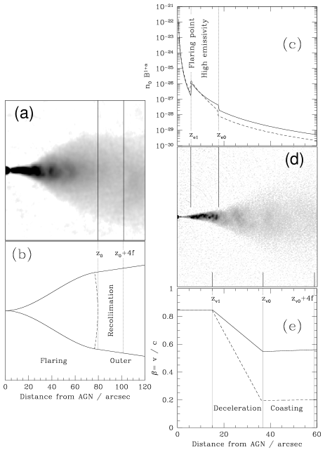
Figure 1: Jet models and fiducial regions for spectral indices. (a) The main jet of NGC 315 at 2.35-arcsec FWHM resolution, indicating the area over which $\alpha_{\rm recoll}$ was evaluated. (b) Sketch showing the flaring and outer regions of the jets in NGC 315 to the same scale as panel (a), but with no bend in the jet. (c) Longitudinal profiles of rest-frame emissivity derived from our model of NGC 315 and plotted against distance from the AGN projected on the plane of the sky. The high-emissivity region is marked. (d) Grey-scale of the main jet at a resolution of 0.4 arcsec FWHM, showing the high-emissivity, deceleration and coasting regions. (e) Longitudinal profiles of velocity derived from our model of NGC 315, with the deceleration and coasting regions marked. In panels (c) and (e), the full and dashed lines apply to the axis and edge of the jet, respectively.

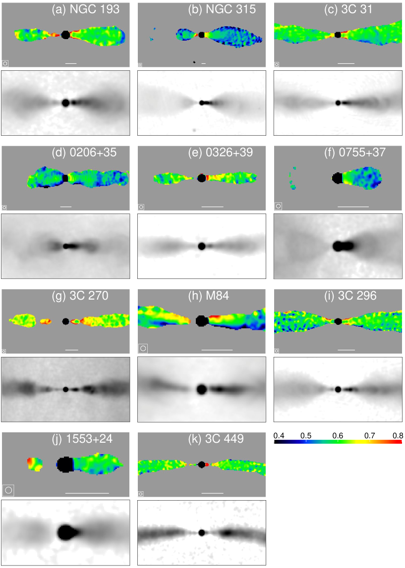
Figure 2: False-colour images of spectral index, $\alpha$ (upper panels) and grey-scales of total intensity (lower panels) at the same resolution. $\alpha$ is in the range 0.4 – 0.8 (as indicated by the labelled wedge) and is plotted wherever $\sigma_{\rm r}<0.03$. The images have been rotated by the angles given in Table 2, so that the approaching jets are always on the right. On the spectral-index plots, the horizontal lines represent distances of 10 arcsec and the restoring beams are shown in the bottom-left-hand corners. Lobe emission has not been subtracted from the $I$ images.

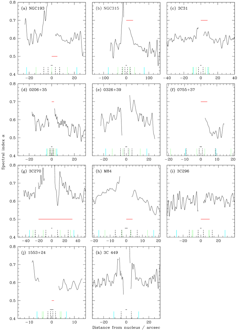
Figure 3: Profiles of spectral index, $\alpha$, along the jets. The brighter (approaching) jet is always on the right. The profiles are derived from the images shown in Fig. 2, along horizontal lines passing through the nuclei (a different position angle was used for the counter-jet of M 84, which is misaligned with the main jet). Profiles are only plotted where $\sigma_{\rm r}\leq 0.03$ and the distance from the core exceeds 2 $\times$ FWHM. The beamwidths (FWHM) are indicated by the horizontal lines centred on distance 0 and $\alpha=0.45$. The vertical dashed black lines represent the extent of the high-emissivity region and the dotted vertical green lines the start and end of rapid deceleration. The vertical full cyan lines show where the jets recollimate. The horizontal red lines plotted at $\alpha=0.5$ or $\alpha=0.7$ show the maximum extent of any detected soft X-ray or optical emission from the jets (Table 3).

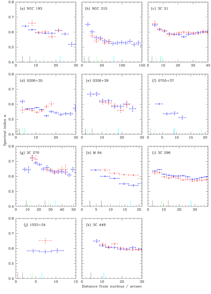
Figure 4: Profiles of integrated spectral index, $\alpha$, along the jets. The spectral indices were calculated from total intensities integrated over points with $\sigma_{\rm r}\leq 0.03$ in boxes of length 2FWHM along the jet axis (horizontal in Fig. 2, starting at 2FWHM from the core. Data are only plotted if there are more than two independent beam areas above the blanking level in the box. Blue full and red dashed symbols represent main and counter-jets, respectively. The fiducial distances are indicated as in Fig. 3.

4 Spectral-index images and profiles

4.1 Images

In Fig. 2 we show false-colour images of spectral index over the range $0.4\leq\alpha\leq 0.8$ for all of the sources, together with grey-scales of total intensity at the same resolution. The images have been rotated by the angles given in Table 2 so as to have the main jets on the right.

Except for the unresolved cores, which are partially optically thick with $\alpha\la 0.3$, the emission typically has $0.7\ga\alpha\ga 0.5$. Significantly higher or lower spectral indices are only found close to the edges of the jets (where small errors in deconvolution, lobe subtraction or image registration can cause large changes in $\alpha$) or in regions of low signal-to-noise ratio. The mean spectral indices of the jets vary over a range of $\approx$0.1, with NGC 315 showing the flattest spectrum and 3C 270 the steepest. The spectral indices of main and counter-jets are usually very similar, with M 84 and 1553+24 the only conspicuous exceptions.

A slight, but significant tendency for the spectral index to decrease away from the AGN is apparent from the images in Fig. 2. The effect is subtle ($\Delta\alpha\la 0.1$) but consistent.

Table 4: Integrated spectral indices for high-emissivity, deceleration, coasting and recollimation regions. (1) source name; (2) rms calibration error for spectral indices $\sigma_{\rm c}$. The remaining columns give the mean spectral indices, $\langle\alpha\rangle$ and their estimated random errors for the four fiducial regions in each jet. Values are not given if one or more of the regions: has too little data of adequate signal-to-noise (NGC 315; 3C 31, 0755+37), is too close to the core (0206+35 and 1553+24) or is undefined (3C 449).

Source	$\sigma_{\rm c}$	High-emissivity				Deceleration				Coasting				Recollimation
		jet		cj		jet		cj		jet		cj		jet		cj
		$\langle\alpha\rangle$	$\pm$	$\langle\alpha\rangle$	$\pm$	$\langle\alpha\rangle$	$\pm$	$\langle\alpha\rangle$	$\pm$	$\langle\alpha\rangle$	$\pm$	$\langle\alpha\rangle$	$\pm$	$\langle\alpha\rangle$	$\pm$	$\langle\alpha\rangle$	$\pm$
NGC 193	0.036	0.64	0.01	0.75	0.05	0.62	0.01	0.63	0.02	0.59	0.01	0.59	0.02	0.58	0.02	0.65	0.03
NGC 315	0.027	0.65	0.01	0.76	0.04	0.60	0.01	0.57	0.01	0.55	0.01	0.55	0.01	0.53	0.01
3C 31	0.017	0.64	0.01	0.64	0.01	0.63	0.01	0.63	0.01					0.60	0.01	0.60	0.01
0206+35	0.036					0.63	0.02	0.56	0.05	0.59	0.03	0.57	0.04	0.56	0.01	0.56	0.01
0326+39	0.023	0.67	0.01	0.60	0.09	0.65	0.01	0.62	0.01	0.60	0.01	0.60	0.01	0.59	0.01	0.57	0.01
0755+37	0.036	0.58	0.01			0.57	0.01
3C 270	0.036	0.67	0.02	0.71	0.03	0.68	0.02	0.67	0.02	0.64	0.02	0.63	0.02	0.63	0.02	0.64	0.02
M 84	0.036	0.64	0.01	0.67	0.02	0.61	0.01	0.63	0.01	0.55	0.01	0.61	0.01	0.55	0.01	0.59	0.01
3C 296	0.034	0.64	0.01	0.62	0.01	0.63	0.01	0.62	0.01	0.60	0.01	0.59	0.01	0.58	0.01	0.57	0.01
1553+24	0.023					0.57	0.02			0.60	0.01	0.61	0.04	0.58	0.01	0.67	0.02
3C 449	0.016	0.68	0.01	0.68	0.03									0.61	0.01	0.61	0.01

4.2 Longitudinal profiles

In order to investigate the spectral gradients in more detail, we have plotted profiles of spectral index along the jets in two representations: as unaveraged slices along the jet ridge-lines to show the level of variation on small as well as large scales (Fig. 3) and as binned averages to reduce random noise and to compare values in the main and counter-jets (Fig. 4). The unbinned profiles are plotted for distances $>$2$f$ from the AGN wherever the rms random error on the spectral index determined from the off-source noise $\sigma_{\rm off}$ (Table 2) is $\sigma_{\rm r}\leq 0.03$. The binned profiles follow the prescription given in Section 2.4.

The clear tendency for the spectra to flatten with distance from the AGN is confirmed, and the binned profiles (Fig. 4) show in addition that the jet and counter-jet spectral indices at the same distance from the AGN are usually very similar. Of the two exceptions noted earlier, M 84 (Fig. 4h) shows an offset between the spectral indices of its jets which results from an instrumental effect (Appendix B) and 1553+24 (Fig. 4j) has a weak counter-jet with measurable spectral index only over a limited range of distance.

The fiducial distances from our jet models (projected on the sky) are plotted in Figs 3 and 4. Most of the spectral flattening with distance from the AGN occurs before the jets recollimate, and appears to be associated with rapid deceleration. The clearest examples are the well-resolved and bright sources NGC 315, 3C 31, 3C 270 and 3C 296 (Figs 4b, c, g and i).

High-frequency ($>$10¹⁴ Hz) emission is seen in many of the main jets and in the counter-jet of 3C 270. Although the data are heterogeneous, with a mixture of optical and X-ray detections and various exposure times, the comparison in Fig. 3 shows that the detected high-frequency emission typically extends roughly as far as the end of the high-emissivity region.

4.3 Spectral indices at fiducial locations

Figure 5: Histograms of spectral indices at different locations, as given in Table 4. (a) high-emissivity; (b) deceleration; (c) coasting; (d) recollimation. The shaded areas represent the main jets. The vertical dotted lines indicate the unweighted means of the distributions, from Table 5.

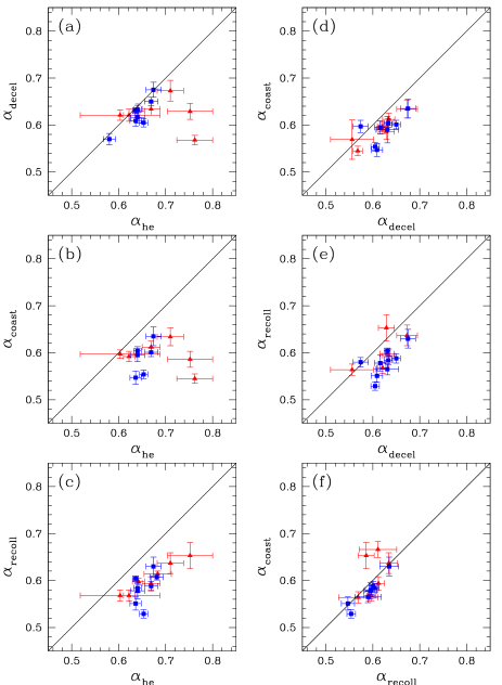
Figure 6: Plots comparing spectral indices at different locations in the same jet. (a) High-emissivity and deceleration. (b) High-emissivity and coasting. (c) High-emissivity and recollimation. (d) Deceleration and coasting. (e) Deceleration and recollimation. (f) coasting and recollimation. Blue squares: main jets; red triangles: counter-jets. The error bars correspond to random errors $\sigma_{\rm r}$ only: calibration errors would be expected to move the point parallel to the line of equality, which is plotted for reference.

Figure 7: Comparison between the main and counter-jet spectral indices, $\alpha_{\rm j}$ and $\alpha_{\rm cj}$ for the four fiducial regions. (a) high-emissivity; (b) deceleration; (c) coasting; (d) recollimation. The error-bars represent the random errors, $\sigma_{\rm r}$.

Table 5: Mean and rms spectral indices for the four fiducial regions, for main and counter-jets separately and for the combination. (1) jet class; (2) location; (3) number of jets; (4) unweighted mean spectral index; (5) measured spectral index rms; (6) rms predicted from the combination of random and calibration errors; (7) standard error on the unweighted mean; (8) mean weighted by random and calibration errors.

. Jet Region $N$ Unweighted Wtd $\langle\alpha\rangle$ $\sigma_{\rm obs}$ $\sigma_{\rm pred}$ $\pm$ $\langle\alpha\rangle$ Main high- 9 0.645 0.028 0.033 0.009 0.650 CJ emiss- 8 0.680 0.054 0.050 0.019 0.668 Both ivity 17 0.662 0.046 0.042 0.011 0.656 Main decel- 10 0.619 0.031 0.034 0.010 0.621 CJ eration 8 0.617 0.035 0.038 0.012 0.618 Both 18 0.618 0.033 0.036 0.008 0.620 Main coast- 8 0.590 0.026 0.036 0.009 0.590 CJ ing 8 0.593 0.026 0.040 0.009 0.590 Both 16 0.592 0.026 0.038 0.007 0.590 Main recoll- 10 0.582 0.027 0.032 0.009 0.589 CJ imation 9 0.607 0.036 0.034 0.012 0.605 Both 19 0.594 0.034 0.033 0.008 0.596

Table 6: Differences between spectral indices integrated over the standard regions. (1) spectral-index combination; (2) number of measurements (main and counter-jets); (3) mean spectral-index difference; (4) rms; (5) standard error on the mean; (6) significance level of correlation between spectral indices at the two locations, from the Spearman rank test.

Location	N	$\langle\Delta\alpha\rangle$	rms	$\pm$	sig
$\alpha_{\rm he}-\alpha_{\rm decel}$	15	0.035	0.053	0.014	77.0
$\alpha_{\rm he}-\alpha_{\rm coast}$	12	0.077	0.058	0.017	18.0
$\alpha_{\rm he}-\alpha_{\rm recoll}$	15	0.067	0.024	0.006	99.9
$\alpha_{\rm decel}-\alpha_{\rm coast}$	15	0.029	0.022	0.006	$>$99.9
$\alpha_{\rm decel}-\alpha_{\rm recoll}$	16	0.037	0.027	0.007	99.7
$\alpha_{\rm coast}-\alpha_{\rm recoll}$	15	0.005	0.028	0.007	99.9

Table 7: Mean differences between the spectral indices of the main and counter-jets at the four fiducial locations. (1) location; (2) mean $\langle\alpha_{\rm cj}-\alpha_{\rm j}\rangle$; (3) standard error on the mean; (4) number of sources; (5) significance level of correlation between $\alpha_{\rm cj}$ and $\alpha_{\rm j}$, according to the Spearman rank test.

Location	$\langle\alpha_{\rm cj}-\alpha_{\rm j}\rangle$	$\pm$	N	sig
High-emissivity	0.027	0.020	8	35.3
Deceleration	-0.015	0.010	8	43.5
Coasting	0.003	0.009	8	68.0
Recollimation	0.019	0.012	9	47.1

Individual integrated spectral indices over the four fiducial areas are given in Table 4, along with rms random errors $\sigma_{\rm r}$ estimated using the prescription in Section 2.4. The rms calibration errors $\sigma_{\rm c}$, which are common to all of the measurements for an individual jet, are also tabulated. $\sigma_{\rm r}\approx 0.01-0.02$ in regions of high signal-to-noise, with significantly larger values primarily in those counter-jets whose high-emissivity regions are both faint and close to a bright core.

Histograms of the distributions are plotted in Fig. 5. These display the progressive decrease of spectral index from high-emissivity through deceleration to coasting regions. There is no evidence of further systematic spectral flattening after recollimation: the distributions for the coasting and recollimation regions are statistically the same (the significance level of the difference is only 28% according to the Kolmogorov-Smirnov test), consistent with very similar spectral-index and error distributions. The histogram for the high-emissivity region (Fig. 5a) is slightly broader than the other three; this is expected from the larger random errors in the counter-jet spectral indices, and the distribution for the main jets alone is narrower.

Statistics of the distributions for the main and counter-jets separately and for the two combined are listed in Table 5. Here, and wherever we quote the error on a mean spectral index, we give the standard error derived from the dispersion in the measurements. The unweighted means are very close to those weighted by the combined (random and calibration) errors. The unweighted mean spectral index for the high-emissivity region, $\langle\alpha_{\rm he}\rangle=0.662\pm 0.011$, is significantly steeper than those for either the coasting or the recollimation regions ($\langle\alpha_{\rm coast}\rangle=0.592\pm 0.007$ and $\langle\alpha_{\rm recoll}\rangle=0.594\pm 0.008$, respectively). The mean for the deceleration region, $\langle\alpha_{\rm decel}\rangle=0.618\pm 0.008$, is in the middle of this range. While both the random and calibration errors contribute to the observed dispersion, any systematic error in the flux-density scale does not. We expect the rms scale error in spectral index to be $<$0.02 (the value corresponding to independent scale errors at 1.4 and 4.9 GHz as given by Perley & Butler 2013).

More accurate measures of the change in spectral index with distance are given by the differences for individual jets, since any scale and calibration errors then cancel out. We plot the combinations of spectral indices at the four standard locations in Fig. 6. All of the combinations show spectral flattening with increasing distance except for the plot of $\alpha_{\rm recoll}$ against $\alpha_{\rm coast}$ (Fig. 6f). In particular, all of the jets have spectra which flatten between the high-emissivity region and both the coasting and recollimation regions (Figs 6b and c). The mean differences are listed in Table 6. By this measure, the spectral flattening between high-emissivity and deceleration regions is not very significant ($2.5\sigma$) and that between coasting and recollimation regions is consistent with zero. The remaining differences show significant flattening ($>$4.5$\sigma$). The most significant difference is between the high-emissivity and recollimation regions, for which $\langle\alpha_{\rm he}-\alpha_{\rm recoll}\rangle=0.067\pm 0.006$, consistent with a constant spectral-index change for all of the 15 jets with measurements at these locations (Fig. 6c). The particularly good agreement between the integrated spectral indices measured for the outer two regions in the same jet, despite the evidence for slight local variations in spectral index associated with total-intensity enhancements (Section 4.5) suggests that the internal errors cannot be much greater than we assume.

The internal consistency of the measurements is extremely good: all of the jets for which we have accurate spectral indices show the same trend. There are a few discrepant points but these all represent faint counter-jets for which the errors in our spectral index estimates are large, so the discrepancies are not significant (Fig. 6). The rms spectral indices predicted by the combination of random and calibration errors, $\sigma_{\rm pred}$, are also close to the observed values (Table 5). More formally, we find that our measurements and error model are consistent with all jets having the same spectral indices at the standard locations: this hypothesis is excluded only at the 73%, 40%, 11% and 74% confidence levels by a $\chi^{2}$ test for the high-emissivity, deceleration, coasting and recollimation regions, respectively. The validity of these confidence levels is, however, almost entirely dependent on the accuracy of our estimate of calibration error: if we have overestimated this, then some intrinsic dispersion in spectral index would be required, albeit limited to $<$0.03 – 0.05 rms even for perfect data.

Fig. 6 also shows strong correlations between the spectral indices measured in the same jet at different locations. The significance levels of these correlations, derived from the Spearman rank test, are given in Table 6. Four of the correlations are significant at $>$99.7% confidence; the exceptions are those between $\alpha_{\rm he}$ and $\alpha_{\rm coast}$ or $\alpha_{\rm decel}$. There are two possibilities: the correlations result from residual calibration errors or the spectral-index evolution of the jets follows a roughly similar trend, but with source-dependent offsets. These cases are not mutually exclusive and are difficult to distinguish, but we note that our assumed 3% calibration error corresponds to an rms spread in spectral index of $\approx$0.03 between 4.9 and 1.4 GHz. This is very close to the rms spread along the line of equality in any of the panels of Fig. 6. If our assumed calibration errors are accurate, then we cannot exclude the possibility that all of the jets have identical spectral indices at the fiducial locations.

4.4 Spectral differences between main and counter-jets

We find no statistically significant differences between the spectral indices of the main and counter-jets at any of the four fiducial locations. The individual values are plotted in Fig. 7 and the mean differences and their errors are given in Table 7. As noted earlier, the only source which shows a consistent offset between the two spectral indices is M 84 (Fig. 4h), but this is almost certainly due to imaging artefacts (Appendix B). The correlations between spectral indices for the main and counter-jets at the fiducial locations are not significant ($\leq$68% using the Spearman rank test; Table 7).

If the spectrum is not a pure power law and the jets are relativistic, then systematic differences are expected between observed spectral indices of approaching and receding jets. We return to this point in Section 5.3.

4.5 Transverse and local spectral-index variations

In detailed studies of 3C 31, NGC 315 and 3C 296 (Laing et al., 2006a, b, 2008b), we drew attention to two additional features of the spectral-index distributions.

Firstly, the spectrum of the main jet in NGC 315 flattens away from its axis (Laing et al., 2006b) as well as with distance from the AGN; the same effect is visible in its counter-jet (Fig. 2b) and, at a low level, on one side of each of the jets in 3C 31 (Laing et al., 2008b, Fig. 2c of the present paper). We have found no similar systematic patterns in the rest of the sample. It is doubtful, however, that we could have reliably detected such a subtle effect in sources with steeper-spectrum lobe emission surrounding the jets given the simplicity of our linear subtraction algorithm (Section 2.3). Of the five sources where lobe emission is undetectable over the region of interest, NGC 315 and (at a much lower level) 3C 31 show the spectral flattening away from the axis mentioned earlier, 0326+39 and 3C 449 have no systematic gradients and 1553+24 is not well enough resolved. The pronounced transverse spectral gradient in NGC 315 therefore seems to be unusual, although we cannot rule out similar effects at a lower level in other sources. This gradient extends over many beam areas at high signal-to-noise (Fig. 2b). In contrast, the narrow rims of steeper-spectrum emission seen close to the cores in NGC 193, 3C 31, 3C 270 and 3C 296 (Figs 2a, c, g, i) occur in regions where the jets are narrow and faint, and are likely to result from small calibration or deconvolution errors affecting the bright cores. Narrow spectral-index features at the faint edges of jets at larger distances from the nucleus are also suspect, particularly in cases where significant lobe emission has been subtracted (e.g. the counter-jet in 0206+35, Fig. 2d).

Secondly, we identified “arcs” – narrow enhancements in total and polarized intensity crossing the jets – in 3C 31 and 3C 296. The two brightest arcs in 3C 31 have slightly ($\Delta\alpha\la 0.05$) flatter spectra than the surrounding emission (Laing et al., 2008b). In 3C 296, the spectrum is flatter in both jets roughly where the more distinct arcs are seen, but the arcs are not recognisable individually on the spectral-index images (Laing et al., 2006a). The remaining small-scale fluctuations visible in Fig. 2 are consistent with noise and calibration errors.

5 Discussion

5.1 A common spectral-index profile?

Our jet models suggest that the flaring region is an approximately homologous structure, in the sense that the width and fiducial distances for emissivity and velocity all scale with the recollimation distance despite the wide range in physical size (the recollimation distance measured along the jet axis, $r_{0}$, ranges from 1.5 kpc in M 84 to 35 kpc in NGC 315). We will discuss these relations in detail elsewhere (Laing & Bridle, in preparation), but the scaling is already evident from Table 3. The spectral indices at our standard locations in the flow show very little dispersion between sources, so they must also follow this scaling, as can be illustrated directly by plotting the spectral index as a function of distance normalized to the size of the flaring region, $z/z_{0}$. In order to remove the confusing effects of scale and calibration errors, we evaluated the differences $\Delta\alpha$ between the binned spectral indices in Fig. 4 and a reference value in the same jet. We took the reference to be $\alpha_{\rm coast}$ ($\alpha_{\rm recoll}$ for 3C 31 and 3C 449, where the former is undefined), forcing the mean profile for each jet to have $\Delta\alpha=0$ at the reference location. The results are shown in Fig. 8. There is a clear trend in the combined data: on average, the spectral index falls from $\Delta\alpha\approx 0.06$ at $z/z_{0}\approx 0.2$ (as close to the flaring point as we can measure) to $\Delta\alpha\approx 0$ at $z/z_{0}\approx 0.8$ (the reference location). This confirms our new result: the variations of spectral index appear to scale with the size of the flaring region in the same way as variations of velocity and emissivity.

Jets evolve in cross-section and velocity as a consequence of mass injection and propagation in external pressure and density gradients (e.g. Laing & Bridle 2002b). Their emissivities are in turn governed by the balance of particle acceleration and energy-loss processes. The most natural way to ensure a common scaling for these quantities is for the acceleration mechanism to depend on flow speed, as we now discuss.

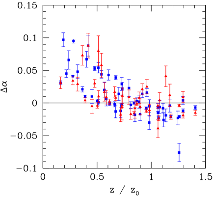
Figure 8: Plot of $\Delta\alpha$ against normalized distance from the AGN. $\Delta\alpha$ is the difference between the spectral index of a bin from Fig. 4 and its mean value in the coasting region (or the recollimation region, if the former cannot be measured; see Table 5). Distance from the AGN, $z$, is normalized by the recollimation distance, $z_{0}$. Blue squares: main jets; red triangles: counter-jets. Data at $z/z_{0}>1.5$ are available only for a few jets and are not plotted. 0755+37 (which has no measured reference spectral index) is also omitted, as are data from upstream of the flaring point in 3C 270 and 3C 449.

5.2 A relation between spectral index and flow speed?

Given that we model the jets as decelerating flows, and that the spectral index decreases monotonically with distance from the AGN in the regions studied here, there must be some relation between $\alpha$ and speed. In order to quantify this relation, we have chosen a representative speed $\beta_{0.5}$ for each source, determined from our model for a streamline half way between the axis and boundary of the jet. Spectral index difference (as in Section 5.1) is plotted against $\beta_{0.5}$ in Fig. 9. There is a clear separation: all points with $\beta_{0.5}>0.5$ have $\Delta\alpha>0$, whereas the mean $\Delta\alpha$ at lower velocity is close to 0.

An upper bound to the sound speed in the jet is that for an ultrarelativistic plasma, $\beta_{\rm s}=3^{-1/2}=0.58$. $\beta_{\rm s}$ may be significantly lower than this limit, particularly if the jet contains appreciable numbers of non-relativistic protons (entrained or part of the initial composition), and may change systematically with position in the jet (Laing & Bridle, 2002b). One possibility is then that the jet composition is dominated by ultrarelativistic leptons and magnetic field with a minor baryonic component and that the spectral index is significantly higher than its asymptotic value of $\langle\alpha\rangle=0.59$ wherever the average flow speed is even slightly supersonic. For the 10 sources we have modelled, the mean velocity at the flaring point is $\beta=0.81$ with an rms of 0.08. This in turn corresponds to a generalized Mach number of ${\cal M}=(\Gamma\beta)/(\Gamma_{\rm s}\beta_{\rm s})=1.95$ for an ultrarelativistic plasma, where $\Gamma_{\rm s}=(1-\beta_{\rm s}^{2})^{-1/2}$. For 3C 31, we found from a conservation-law analysis that the flow throughout the jet base was transonic everywhere, with the Mach number decreasing from ${\cal M}\approx 2$ to ${\cal M}\approx 1$, despite the increasing mass load (Laing & Bridle, 2002b). Any shocks in this flow regime must be weak.

An alternative possibility is that the sound speeds are much lower than the ultrarelativistic limit, in which case larger Mach numbers are possible for the flow.

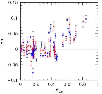
Figure 9: Plot of $\Delta\alpha$ against jet flow velocity. $\Delta\alpha$ is the difference between the spectral index of a bin from Fig. 4 and its mean value in the coasting region (or the recollimation region, if the former cannot be measured; see Table 5). The velocity $\beta_{0.5}$ is that for a streamline mid-way between the axis and the edge of the jet, from our model fits. Blue squares: main jets; red triangles: counter-jets. We have not plotted the inner two bins for the main jet of 3C 270, as these include significant emission from upstream of the flaring point. 0755+37 (no reference spectral index) and 3C 449 (no velocity model) are also omitted.

5.3 Constraints on particle acceleration

We first estimate some fiducial numbers for magnetic fields, for the radiating electron Lorentz factors and for energy loss timescales. The on-axis magnetic-field strengths derived from our emissivity models are $\approx 2-9$ nT at the flaring point and $\approx 0.3-2$ nT at recollimation. The spectrum of synchrotron emission from a single electron is quite broad, but a characteristic frequency is $\nu\approx\gamma^{2}\nu_{\rm g}$, where $\gamma$ is the electron Lorentz factor and $\nu_{\rm g}=eB/2\pi m_{\rm e}$ is the gyro frequency. The corresponding Lorentz factor ranges for electrons radiating at 1.4 – 8.5 GHz are $2000\la\gamma\la 10000$ at the flaring point and $5000\la\gamma\la 30000$ at recollimation. The synchrotron loss timescale is

$$E/(-dE/dt)=\frac{3m_{\rm e}c\mu_{0}}{2\sigma_{\rm T}B^{2}\gamma}$$

which ranges from $6\times 10^{5}$ to $9\times 10^{7}$ yr for emission at 8.5 GHz.

A simple picture in which relativistic electrons are accelerated in the high-emissivity region and then passively advected along the jet, suffering radiative and adiabatic losses as they go, is not consistent with the spectral flattening we observe: radiative losses cause the spectrum to steepen at high energies. Even if the radiating particles are advected down the jet in a constant magnetic field, then the observed frequency spectrum would appear to steepen with distance. In fact, the magnetic field is likely to decrease away from the AGN as a consequence of flux-freezing in a expanding flow. The consequent rapid decrease may be partially compensated by deceleration, shear or turbulent amplification, but (as mentioned earlier) the equipartition field strength still falls by a factor of $\approx$5 – 10 between the flaring point and recollimation. At a fixed frequency, we therefore observe higher-energy electrons and the steepening would be more pronounced. In any case, the minimum loss timescale for X-ray synchrotron emission is $\approx$100 yr for our assumed field strengths and a photon energy of 1 keV. This corresponds to a flow distance of $\approx 30/\beta$ pc (much smaller than the size of a typical jet base), so distributed reacceleration of radiating electrons throughout the regions we observe in FR I jets is unavoidable. Independent evidence for ongoing acceleration comes from modelling of radio brightness and polarization evolution along the jets: additional electrons are also required to offset the effects of adiabatic losses even at energies where the effects of synchrotron cooling are small (Laing & Bridle, 2004). We must therefore attribute the change in characteristic radio spectral index along the jets to the underlying acceleration mechanism rather than to the combined effects of synchrotron and adiabatic losses. Although downward curvature at high frequencies is seen in the broad-band spectra of jet bases (Evans et al., 2005; Hardcastle et al., 2001, 2005; Lanz et al., 2011; Perlman & Wilson, 2005; Perlman et al., 2010; Worrall et al., 2010; Harwood & Hardcastle, 2012), the break frequencies are typically $\ga 10^{12}$ Hz, well above the range considered here.

We have measured the spatial variation of the slope of the radiation spectrum over fixed ranges of observed frequency. In order to characterize the particle-acceleration mechanism, we need to derive the slope of the energy spectrum over a fixed (or, at least, known) energy range. Unless the spectrum is a perfect power law, this presents several complications.

1. There is a known correction factor of $1+z$ for the source redshift.

2. We infer relativistic flow speeds for the jets, so the ratio of observed and emitted frequencies ($\nu_{\rm obs}/\nu_{\rm em}=D$, where $D$ is the Doppler factor) may differ significantly from unity. The emitted frequencies for the approaching and receding jets also differ systematically, but can be calculated from our jet models.

3. As mentioned earlier, the magnetic field strength is likely to decrease away from the AGN along the jet, so emission at a fixed frequency is generated by higher-energy electrons at larger distances. The evolution of field strength with distance is subject to uncertain and mutually contradictory assumptions such as equipartition with relativistic particle energy density or flux freezing.

The correction for redshift is small for these nearby sources (Table 1) and it is constant over both jets, so we can ignore it by comparison with the other two effects, which we consider in turn.

The angles to the line of sight derived from our models range from $\theta=25^{\circ}$ to $\theta=76^{\circ}$ and the maximum velocities over the regions we measure spectral indices are in the range $0.75<\beta<0.95$. For constant-velocity, antiparallel flows, the Doppler factors for the approaching and receding jets are:

$$D_{\rm j} = [\Gamma(1-\beta\cos\theta)]^{-1}$$

$$D_{\rm cj} = [\Gamma(1+\beta\cos\theta)]^{-1}$$

If the energy spectrum deviates from a pure power law, but is the same at a given distance from the AGN in both jets, then we would expect a systematic dependence of spectral index difference $\alpha_{\rm cj}-\alpha_{\rm j}$ on the ratio of Doppler factors $D_{\rm j}/D_{\rm cj}$. The maximum effect for our data should occur close to the flaring point, where the velocities are highest, and is in principle very significant for our sample: the maximum predicted ratio (for 1553+24) is $D_{\rm j}/D_{\rm cj}\approx 13$. Two problems make the effect hard to observe: (a) the largest Doppler factor ratios occur at small angles to the line of sight, so projection makes it difficult to resolve the flaring point from the AGN and (b) if $D_{\rm cj}$ is small, the counter-jet emission is faint and errors on its spectral index are large. As a consequence, we have only been able to measure spectral-index differences over the range $1<D_{\rm j}/D_{\rm cj}<3.5$ for any of the fiducial regions, and those close to the AGN are less well determined. We see no systematic trend in plots of $\alpha_{\rm cj}-\alpha_{\rm j}$ against $D_{\rm j}/D_{\rm cj}$ for either the high-emissivity or coasting regions.

If all jets have the same electron energy spectrum which flattens with increasing energy, then there is a natural explanation for the observed spectral gradients, since the magnetic-field strength must decrease away from the AGN. It seems implausible, however, that this (rather subtle) spectral flattening would occur in precisely the same observed frequency range for all of the jets in our sample, despite the range of field strengths and Doppler factors. The flattening cannot continue over a large energy range without violating constraints from broad-band observations (e.g. Hardcastle et al. 2002, 2005). Finally, it is unclear what mechanism could cause the flattening. This possibility should be tested using accurate measurements of jet spectra over a much larger frequency range, but we consider it to be very unlikely.

The particle acceleration mechanism(s) at work in FR I jets must therefore satisfy the following constraints:

1. The electron energy spectrum can be modelled as a pure power law with spatially-varying mean index $\langle p\rangle=2\langle\alpha\rangle+1$ restricted to the range $2.18\leq\langle p\rangle\leq 2.32$ (Table 5). The characteristic electron Lorentz factor range probed by our observations is $2000\la\gamma\la 30000$, given the assumptions made earlier.

2. The energy spectrum flattens with distance from the AGN, from $\langle p\rangle=2.32$ in the high-emissivity region to $\langle p\rangle=2.18$ in the coasting and recollimation regions.

3. By the argument of Section 5.2 (Fig. 9), $p$ may be determined by the characteristic bulk flow speed: a change in $\langle p\rangle$ from 2.32 to 2.18 being associated with a deceleration from $\beta\approx 0.8$ to $\beta\la 0.5$.

4. The mechanism responsible for the steeper energy spectrum in the high-emissivity regions must be capable of accelerating electrons to Lorentz factors of $\gamma\approx 10^{8}$, as demonstrated by the detection of X-ray emission in many cases (Table 3, Fig. 3). X-ray and/or optical emission is typically seen from the high-emissivity region of the brighter (approaching) jet; in some cases it extends slightly beyond the end of the high-emissivity region, but never beyond the end of deceleration. In the well-observed brighter jets of 3C 31 and NGC 315, the ratio of X-ray to radio emission decreases with distance from the AGN (Laing et al., 2008a). This decrease coincides with the spectral flattening we observe in the radio band and with deceleration.

5. The high-frequency spectrum at larger distances from the AGN (where we infer flatter energy spectra) is not known in most cases. The approaching jet of 3C 31 is detected at 8 $\mu$m wavelength out to a distance of $\approx$25 arcsec (Lanz et al., 2011), implying that acceleration of electrons to $\gamma\approx 10^{5}-10^{6}$ (but not much higher) can occur after deceleration and recollimation.

6. Acceleration is distributed, rather than being associated with rare, localized, prominent brightness enhancements.

5.4 Shock acceleration

First-order Fermi acceleration is thought to be the dominant particle acceleration mechanism at collisionless MHD shocks and there is an extensive literature about this process (see Summerlin & Baring 2012 for a comprehensive list of references). It is also the only process for which there are comprehensive predictions of the energy index under different physical conditions, as we now discuss.

5.4.1 Non-relativistic shocks

Early work (e.g. Bell 1978; Blandford & Ostriker 1978) established that a power-law energy spectrum with index $p=2$ ($\alpha=0.5$) is produced by strong, non-relativistic shocks in the test-particle approximation. This value is inconsistent with our results. Steeper spectra can in principle be produced in weaker shocks: $p=(r+2)/(r-1)$, where $r$ is the velocity compression ratio, and $1<r\leq 4$. There is then no obvious reason for $p$ to have a narrow range, however, as pointed out by Young et al. (2005).

5.4.2 The ultrarelativistic limit

For ultrarelativistic parallel shocks (i.e. those in which the magnetic field is parallel to the shock normal) in which particles experience frequent small-angle scattering, a power-law energy spectrum with $p=2.23$ ($\alpha=0.615$) is produced. This result has been found both analytically (Kirk et al., 2000) and numerically (e.g. Bednarz & Ostrowski 1998; Ellison & Double 2004; Summerlin & Baring 2012). The coincidence between the predicted spectral index and the value of 0.62 we found for three sources in our earlier work (Laing et al., 2008a) led us to wonder whether the ultrarelativistic limit might be relevant at the flaring point. This was puzzling, as the asymptotic value is approached only for shock Lorentz factors $\Gamma\ga 10$ and we infer $\Gamma\la 2$ downstream of the flaring point. On the revised flux-density scale of Perley & Butler (2013), however, the inferred spectra are slightly but significantly steeper, with $\langle\alpha\rangle=0.66\pm 0.01$ in the high-emissivity region for the full sample. Given this discrepancy and the velocities $\beta\la 0.9$ that we infer downstream of the flaring point in FR I jets, it now seems even less likely that the ultrarelativistic limit is relevant to FR I jet bases, although a spectral index of 0.62 is only marginally inconsistent with our result if the rms error due to uncertainties in the flux-density scale is as high as 0.02. Closer to the nucleus, we have no good estimates of the flow Lorentz factor, although Perlman et al. (2011) estimate $\Gamma\approx 4-5$ for the M 87 jet at knot HST-1.

5.4.3 Mildly relativistic shocks

The case of mildly relativistic shocks has been addressed using Monte Carlo methods in the test-particle limit for oblique shocks (Ellison & Double, 2004; Summerlin & Baring, 2012) and in the non-linear case for parallel shocks (Ellison & Double, 2002). These studies show that mildly relativistic shocks can generate a wide variety of power-law slopes for the energy spectrum, depending on the obliquity of the field in the shocks and the nature of the scattering as well as the shock speed (Summerlin & Baring, 2012). Our observations require a narrow range of energy indices, with a slight dependence on mean flow (and therefore shock) velocity. The case which comes closest to meeting these requirements is that of a mildly relativistic velocity upstream of the shock front in the Bohm limit of frequent small-angle scatterings with a mean free path $\lambda$ close to the electron gyro-radius $r_{\rm g}$ (Summerlin & Baring, 2012, Figs 7 and 8). The dependence of $p$ on field obliquity is also weak under these circumstances. The case of an upstream flow velocity $\beta_{\rm u}=0.71$, a velocity compression ratio of $r=3.02$ and a sonic Mach number ${\cal M}=2.6$ gives $2.35\leq p\leq 2.5$, depending on obliquity (Summerlin & Baring, 2012, Fig. 8); for $\beta_{\rm u}=0.1$ and $r=4$, the range is $2\leq p\leq 2.04$ (Summerlin & Baring, 2012, Fig. 7), close to the limit of $p=2$ for a non-relativistic shock. We suggest that these two cases might bracket the range of physical conditions in FR I jet bases, the velocities in the first case being slightly too fast for the flaring point, while those in the second case are too slow for the flow after recollimation, which appears to remain significantly relativistic in most cases. It is plausible that the upstream fluid velocities in the shock rest frame are in the appropriate range, for example if the shocks are stationary or moving slowly in the observed frame, and that there is a range of field obliquities.

5.5 What are the particle acceleration mechanisms?

The first-order Fermi process at mildly relativistic shocks in the limit $\lambda\approx r_{\rm g}$ appears capable of generating energy spectra with the correct indices and of accounting (at least qualitatively) for their variations along the jets. One possibility, therefore, is that this is the sole acceleration mechanism. A potential difficulty, however, is the distributed nature of the acceleration required to power the X-ray emission, which cannot be restricted to a few localized shock sites: instead, a network of shocks extending over a substantial distance along the jet appears to be required. Such shock networks could be identified with the complex, non-axisymmetric brightness structure in the high-emissivity region (e.g. Fig. 1d) or with the arcs observed crossing the jets at larger distances in some sources (Laing et al., 2006a, 2008b). Efficient deceleration of the jet by entrainment probably requires a transonic flow in which any shocks would be very weak, however (Bicknell, 1994; Laing & Bridle, 2002b).

The most likely alternative to a pervasive shock network is that there are two distinct acceleration mechanisms operating in these jets.

1. The first mechanism (which could again be diffusive shock acceleration) dominates wherever the flow velocity $\beta\ga 0.5$ and in particular in the high-emissivity region. It can accelerate electrons up to Lorentz factors $\gamma\approx 10^{7}-10^{8}$, enabling them to emit X-ray synchrotron radiation, and has a characteristic energy index $p=2.32$ over the energy range we sample.

2. A second mechanism with a lower characteristic energy index $p=2.18$ becomes important when the flow velocity falls below $\beta\approx 0.5$, and dominates after deceleration. Gradual shear acceleration (Rieger & Duffy, 2004, 2006) is a plausible candidate, as our jet models show that there are transverse velocity gradients in these regions. We originally favoured this idea for NGC 315 on the grounds that the spectrum flattens away from the jet axis precisely where we infer velocity gradients (Laing et al., 2006b), but this effect seems not to be general (Section 4.5). Second-order Fermi acceleration by plasma turbulence is a possible alternative mechanism.

The existence of two different acceleration mechanisms in FR I jet bases has also been suggested based on evidence from high-resolution observations of X-ray, optical and radio emission from the nearest examples, Centaurus A (Hardcastle et al., 2003; Goodger et al., 2010) and M 87 (Perlman & Wilson, 2005; Perlman et al., 2011). For Cen A, Goodger et al. (2010) suggest that stationary, X-ray-emitting knots are formed when lumps of dense material (e.g. molecular clouds or stars with high mass-loss rates) penetrate the jet, resulting in strong shocks with long-lived particle acceleration up to high Lorentz factors. Conversely, knots emitting only in the radio band (which often have high speeds) would be formed by weak shocks where no particles are accelerated to X-ray emitting energies. The proportion of radio emission from the two processes changes systematically with distance from the AGN. It is not known whether there is a systematic difference in the radio spectra for the two types of knot, as would be expected if the difference is related to the spectral gradients we have discussed.

6 Summary

The principal observational results from our imaging of jet base spectra for a sample of 11 FR I radio galaxies over the frequency range 1.4 – 8.5 GHz are as follows.

1. We find a narrow range of spectral indices, $\alpha$, with the mean values at our fiducial locations ranging from 0.66 to 0.59. The dispersion between sources is consistent with our error model.

2. The radio spectral indices decrease (i.e., the spectra flatten) with distance from the nucleus on the scales we have studied.

3. This spectral flattening occurs between the flaring point and the end of rapid deceleration as determined from our modelling of the jets as decelerating relativistic flows; thereafter the spectral index is constant until after the jets recollimate.

4. The spectral flattening is highly significant: the average decrease in spectral index between the high-emissivity region immediately downstream of the flaring point and just after the jet recollimates is $0.067\pm 0.006$ and all jets for which we have data show spectral flattening between these two locations.

5. The mean spectral index for the high-emissivity region is $\langle\alpha\rangle=0.662\pm 0.011$; coasting and recollimation regions have $\langle\alpha\rangle=0.592\pm 0.007$ and $0.594\pm 0.008$, respectively.

6. There are no significant differences between the spectral indices of main and counter-jets at the same distance from the nucleus.

7. All of the jets show essentially the same variation of spectral index with distance from the nucleus when the distances are normalized to the observed recollimation scale.

8. The steeper spectra close to the jet flaring points appear to be associated with bulk flow speeds $\beta\ga 0.5$.

9. The measured values of $\alpha$ correspond to indices of $p=2.18-2.32$ for the electron energy spectrum over a Lorentz factor range of 2000 – 30000, assuming equipartition magnetic fields.

The range of observed spectral indices and the inferred dependence on velocity could result from first-order Fermi acceleration by mildly relativistic shocks, in the limit that the scattering mean free path is close to the electron gyro-radius. Such a model would require a network of shocks in order to produce distributed particle acceleration.

Alternatively, there may be two acceleration mechanisms. The first can accelerate electrons to Lorentz factors of $10^{7}-10^{8}$, is dominant for bulk flow speeds $\beta\ga 0.5$ close to the flaring point and has p = 2.32 at low energies. The second dominates at slower flow speeds and thus at larger distances, has $p=2.18$ and a lower maximum energy. Shock acceleration is (again) a good candidate for the first mechanism

In order to distinguish between these (and other) alternatives, accurate, well-sampled, spatially-resolved spectra over a very wide frequency range (ideally from low-frequency radio to X-ray) are required. More detailed predictions of the energy spectra produced by various acceleration mechanisms, especially for Fermi acceleration by magnetized, mildly relativistic shocks in the Bohm limit, would also be valuable.

Appendix A Archival VLA observations of 0326+39 and 1553+24

The observations and data reduction for the images of 0326+39 and 1553+24 in the 4.5 – 5.0 and 1.3 – 1.7 GHz bands have not been documented elsewhere, so we summarize them here. Data were retrieved from the VLA archive, calibrated and imaged using the aips package, following standard procedures essentially as described by Laing et al. (2011). 3C 48 or 3C 286 were used as primary amplitude calibrators. All sources were self-calibrated and data from multiple array configurations were combined. The final images were made using a multi-scale clean algorithm (Greisen et al., 2009).

For 1553+24, we chose not to make images at 1464.9 MHz, as the available A-configuration data at this frequency were badly affected by interference. We also analysed other archival datasets at 1665 and 1415 MHz, but these were not observed in all relevant configurations and did not help to improve the accuracy of the final spectral-index image.

Table 8: Journal of VLA observations. (1) source name; (2) date of observation; (3) VLA configuration (H denotes a hybrid configuration, as described by Bridle et al. 1991); (4) and (5) frequencies (MHz); (6) bandwidth (MHz); (7) duration (min); (8) key to proposal code and reference.

0326+39	1980 04 15	H	4885.1		50	772	1
	1997 12 14	D	4885.1	4835.1	50	11	2
	1997 12 17	D	4885.1	4835.1	50	46	2
	1998 12 04	C	4885.1	4835.1	50	34	2
	1998 12 11	C	4885.1	4835.1	50	13	2
	1997 12 14	D	1385.1	1464.9	50	14	2
	1997 12 17	D	1385.1	1464.9	50	21	2
	1998 04 28	A	1385.1	1464.9	50	98	2
	1998 07 23	B	1385.1	1464.9	50	129	2
	1998 12 04	C	1414.9	1464.9	50	25	2
	1998 12 11	C	1385.1	1464.9	50	8	2
1553+24	1985 07 16	C	4885.1	4835.1	50	15	3
	1987 11 29	B	4885.1	4835.1	50	103	4
	1992 03 19	C	4885.1	4835.1	50	25	5
	1998 11 28	C	4885.1	4835.1	50	33	6
	1998 12 20	C	4885.1	4835.1	50	25	6
	1999 01 18	C	4885.1	4835.1	50	24	6
	1999 04 15	D	4885.1	4835.1	50	52	6
	2000 02 09	B	4885.1	4835.1	50	103	6
	1998 11 28	C	1385.1		50	15	6
	1998 12 20	C	1385.1		50	12	6
	1999 01 18	C	1385.1		50	12	6
	1999 09 20	A	1385.1		50	140	6
	2000 02 09	B	1385.1		50	64	6

Proposal codes and references:

1 BRID (Bridle et al., 1991)

2 AR386 (unpublished)

3 AM154 (Morganti et al., 1987)

4 AM222 (unpublished)

5 AM364 (Morganti et al., 1997)

6 AR402 (Young et al., 2005)

Appendix B Notes on individual sources

NGC 315

A detailed study of the spectral-index distribution was given by Laing et al. (2006b). The spectrum of the jets is unusually flat, although less extreme than in our earlier work after correction of the flux-density scale.

3C 31

A detailed study of the spectral index distribution was presented by Laing et al. (2008b). The coasting region is not defined, as the deceleration region extends slightly beyond recollimation.

0206+35

Spectral-index images of the whole source were shown by Laing et al. (2011) and for the jets alone (with a less stringent blanking criterion than used here) by Laing & Bridle (2012). A residual calibration error caused a high-frequency ripple in spectral index transverse to the jet axis, visible in the brighter parts of the jets (Fig. 3d). The amplitude of this ripple is roughly $\Delta\alpha\approx 0.01$, and we do not believe that it has any systematic effect on our results. The high-emissivity region is not well enough resolved from the core for us to determine accurate spectral indices. We have included the part of the jet and counter-jet emission that we model as backflow (Laing & Bridle, 2012) in the binned spectral-index profiles and averages, since these are very hard to separate from the outflow component at 1.2-arcsec resolution.

0326+39

Bridle et al. (1991) show spectral-index profiles derived from lower-resolution images at 1.5 and 4.9 GHz.

0755+37

Spectral-index images of the whole source and for the jets have been presented elsewhere, as for 0206+35 (Laing et al., 2011; Laing & Bridle, 2012). Only the main jet has enough unblanked emission for us to derive a reliable spectral index. We considered using lower-resolution images to improve the signal-to-noise ration, but lobe subtraction was problematic. Although we model the jets as a mixture of outflow and backflow (Laing & Bridle, 2012), the spectral indices in the present paper are dominated by the outflow component.

3C 270

A detailed discussion of the radio structure, spectral index and magnetic-field structure of 3C 270 will be given by Laing, Guidetti & Bridle (in preparation). The average spectral index of the jets of 3C 270 is unusually high. This is the only source where we can measure the spectral index accurately upstream of the flaring point. The abrupt steepening of the spectrum of the main jet from $\alpha\approx 0.55$ to $\alpha\approx 0.7$ between distances of $\approx$9 and $\approx$12 arcsec from the nucleus is seen most clearly in the unbinned profile (Fig. 3g). Given that our model fits give an unusually large range for the flaring-point position (6.5 – 11.5 arcsec in projection), it is likely that the steepening occurs exactly at the flaring point. The location of the spectral steepening is blurred by the binning in Fig. 4(g).

M 84

There are significant artefacts on the 1413-MHz image of M 84, caused by a combination of poor spatial-frequency coverage, the proximity of the bright confusing source M 87 and the displacement of the pointing centre in some of the observations (Laing et al., 2011). There are ripples of amplitude $\Delta\alpha\approx 0.1$ and wavelength ranging from $\approx$3 to $\approx$15 arcsec on the spectral-index image (Laing et al., 2011, fig. 9c). These are aligned in the NS direction (roughly parallel to the jets).

3C 296

We have given a comprehensive discussion of the spectral-index distribution of 3C 296 elsewhere (Laing et al., 2006a, 2011).

1553+24

Young et al. (2005) showed images of this source (we include some of their visibility data) but did not discuss its spectrum quantitatively. The high-emissivity region is too close to the core for accurate spectral-index measurements to be made; this is the one source where it does not overlap with the deceleration region. The signal-to-noise ratio in the counter-jet is low.

3C 449

The spectra of the jets in this source were measured by Feretti et al. (1999) and studied in detail by Katz-Stone & Rudnick (1997). Our measured spectral indices are consistent with the mean value $\langle\alpha\rangle=0.58\pm 0.02$ between 4.985 and 8.4 GHz with 2.5-arcsec resolution quoted by Feretti et al. (1999) from the same visibility data once we account for recalibration. Note that the steep-spectrum emission surrounding the jets does not start until well outside our region of interest (Katz-Stone & Rudnick, 1997). The inner jets are very symmetrical, indicating that they are almost precisely in the plane of the sky. For this reason, we cannot model the jet velocity field, and have no good estimate of the deceleration scale, although by analogy with other sources it is likely to be $\la$10 arcsec.

References

- (1)
- Abdo et al. (2011) Abdo A.A., et al., 2011, ApJ, 727, 129
- Abreu et al. (2010) Abreu P., et al., 2010, Astroparticle Physics, 34, 314
- Baars et al. (1977) Baars J.W.M., Genzel R., Pauliny-Toth I.I.K., Witzel, A., 1977, A&A, 61, 99
- Bednarz & Ostrowski (1998) Bednarz J., Ostrowski M., 1998, Physical Review Letters, 80, 3911
- Bell (1978) Bell A.R., 1978, MNRAS, 182, 147
- Bicknell (1994) Bicknell G.V., 1994, ApJ, 422, 542
- Birk & Lesch (2000) Birk G.T., Lesch H., 2000, ApJ, 530, L77
- Blandford & Ostriker (1978) Blandford R.D., Ostriker J.P., 1978, ApJ, 221, L29
- Bridle et al. (1991) Bridle A.H., Baum S.A., Fomalont E.B., Parma P., Fanti R., Ekers R.D., 1991, A&A, 245, 371
- Canvin & Laing (2004) Canvin J.R., Laing R.A., 2004, MNRAS, 350, 1342
- Canvin et al. (2005) Canvin J.R., Laing R.A., Bridle A.H., Cotton W.D., 2005, MNRAS, 363, 1223
- Cornwell & Evans (1985) Cornwell T.J., Evans K.F., 1985, A&A, 143, 77
- Croston et al. (2003) Croston J.H., Birkinshaw M., Conway E., Davies R.L., 2003, MNRAS, 339, 82
- de Vaucouleurs et al. (1991) de Vaucouleurs G., de Vaucouleurs A., Corwin H.G. Jr., Buta R.J., Paturel G., Fouqué P., 1991, Third Reference Catalogue of Bright Galaxies, Springer, New York
- Ellison & Double (2002) Ellison D.C., Double G.P., 2002, Astroparticle Physics, 18, 213
- Ellison & Double (2004) Ellison D.C., Double G.P., 2004, Astroparticle Physics, 22, 323
- Evans et al. (2005) Evans D.A., Hardcastle M.J., Croston J.H., Worrall D.M., Birkinshaw M., 2005, MNRAS, 359, 363
- Falco et al. (1999) Falco E.E., et al., 1999, PASP, 111, 438
- Fanaroff & Riley (1974) Fanaroff B.L., Riley J.M., 1974, MNRAS, 167, 31p
- Feretti et al. (1999) Feretti L., Perley R., Giovannini, G., Andernach H., 1999, A&A, 341, 29
- Goodger et al. (2010) Goodger J.L., et al., 2010, ApJ, 708, 675
- Greisen et al. (2009) Greisen E.W., Spekkens K., van Moorsel G.A., 2009, AJ, 137, 4718
- Guidetti et al. (2010) Guidetti D., Laing R.A., Murgia M., Govoni F., Gregorini L., Parma P., 2010, A&A, 514, A50
- Hardcastle et al. (2001) Hardcastle M.J., Birkinshaw M., Worrall D.M., 2001, MNRAS, 326, 1499
- Hardcastle et al. (2002) Hardcastle M.J., Worrall D.M., Birkinshaw M., Laing, R.A., Bridle A.H., 2002, MNRAS, 334, 182
- Hardcastle et al. (2005) Hardcastle M.J., Worrall D.M., Birkinshaw M., Laing R.A., Bridle A.H., 2005, MNRAS, 358, 843
- Hardcastle et al. (2003) Hardcastle M.J., Worrall D.M., Kraft R.P., Forman W.R., Jones C., Murray S.S., 2003, ApJ, 593, 169
- Hardcastle et al. (2007) Hardcastle, M. J., et al., 2007, ApJ, 670, L81
- Harris et al. (2002) Harris D.E., Finoguenov A., Bridle A.H., Hardcastle M.J., Laing R.A., 2002, ApJ, 580, 110
- Harwood & Hardcastle (2012) Harwood J.J., Hardcastle M.J., 2012, MNRAS, 423, 1368
- Katz-Stone & Rudnick (1997) Katz-Stone D.M., Rudnick L., 1997, ApJ, 488, 146
- Katz-Stone et al. (1993) Katz-Stone D.M., Rudnick L., Anderson M.C., 1993, ApJ, 407, 549
- Kharb et al. (2012) Kharb P., O’Dea C.P., Tilak A., Baum S.A., Haynes E., Noel-Storr J., Fallon C., Christiansen K., 2012, ApJ, 754, 1
- Kirk et al. (2000) Kirk J.G., Guthman A.W., Gallant Y.A., Achterberg A., 2000, ApJ, 542, 235
- Laing (2002) Laing R.A., 2002, MNRAS, 329, 417
- Laing & Bridle (2002a) Laing R.A., Bridle A.H., 2002a, MNRAS, 336, 328
- Laing & Bridle (2002b) Laing R.A., Bridle A.H., 2002b, MNRAS, 336, 1161
- Laing & Bridle (2004) Laing R.A., Bridle A.H., 2004, MNRAS, 348, 1459
- Laing & Bridle (2012) Laing R.A., Bridle A.H., 2012, MNRAS, 424, 1149
- Laing et al. (2008a) Laing R.A., Bridle A.H., Cotton W.D., Worrall D.M., Birkinshaw M., 2008a, Rector T.A., De Young D.S., eds, ASP Conf. Series 386, Extragalactic Jets: Theory and Observation from Radio to Gamma Ray, ASP, San Francisco, p. 110
- Laing et al. (2008b) Laing R.A., Bridle A.H., Parma P., Feretti L., Giovannini G., Murgia M., Perley, R.A., 2008b, MNRAS, 386, 657
- Laing et al. (2006a) Laing R.A., Canvin J.R, Bridle A.H. Hardcastle, M.J., 2006a, MNRAS, 372, 510
- Laing et al. (2006b) Laing R.A., Canvin J.R, Cotton W.D., Bridle A.H., 2006b, MNRAS, 368, 48
- Laing et al. (2011) Laing R.A., Guidetti D., Bridle A.H., Parma P., Bondi M., 2011, MNRAS, 417, 2789
- Lanz et al. (2011) Lanz L., Bliss A., Kraft R.P., Birkinshaw M., Lal D.V., Forman W.R., Jones C., Worrall D.M., 2011, ApJ, 731, 52
- Leahy & Perley (1991) Leahy J.P., Perley R.A., 1991, AJ, 102, 537
- Lemoine & Pelletier (2003) Lemoine M., Pelletier G., 2003, ApJ, 589, L73
- Miller et al. (2002) Miller N.A., Ledlow M.J., Owen F.N., Hill J.M., 2002, AJ, 123, 3018
- Morganti et al. (1987) Morganti R., Fanti C., Fanti R., Parma P., de Ruiter H.R., 1987, A&A, 183, 203
- Morganti et al. (1997) Morganti R., Parma P., Capetti A., Fanti R., de Ruiter H.R., Prandoni I., 1997, A&AS, 126, 335
- Ogando et al. (2008) Ogando R.L.C., Maia M.A.G., Pellegrini P.S., da Costa L.N., 2008, AJ, 135, 2424
- Parma et al. (2003) Parma P., de Ruiter H.R., Capetti A., Fanti R., Morganti R., Bondi M., Laing R.A., Canvin J.R., 2003, A&A, 397, 127
- Perley & Butler (2013) Perley R.A., Butler B.J., 2013, ApJS, in press, arXiv:1211.1300
- Perlman et al. (1999) Perlman E.S., Biretta J.A., Zhou F., Sparks, W.B., Macchetto F.D., 1999, AJ, 117, 2185
- Perlman & Wilson (2005) Perlman E.S., Wilson, A.S., 2005, ApJ, 627, 140
- Perlman et al. (2010) Perlman E.S. et al., 2010, ApJ, 708, 171
- Perlman et al. (2011) Perlman E.S. et al., 2011, ApJ, 743, 119
- Petrosian (2012) Petrosian V., 2012, Space Science Reviews, 173, 535
- Rieger & Duffy (2004) Rieger F.M., Duffy P., 2004, ApJ, 617, 155
- Rieger & Duffy (2006) Rieger F.M., Duffy P., 2006, ApJ, 652, 1044
- Smith et al. (2000) Smith, R.J., Lucey, J.R., Hudson, M.J., Schlegel, D.J., Davies, R.L., 2000, MNRAS, 313, 469
- Stawarz & Ostrowski (2002) Stawarz L., Ostrowski M., 2002, ApJ, 578, 763
- Summerlin & Baring (2012) Summerlin E.J., Baring M.G., 2012, ApJ, 745, 63
- Trager et al. (2000) Trager S.C., Faber S.M., Worthey G., Gonzalez J.J., 2000, AJ, 119, 1645
- Weiland et al. (2011) Weiland J.L., et al., 2011, ApJS, 192, 19
- Worrall et al. (2001) Worrall D.M., Birkinshaw M., Hardcastle M.J., 2001, MNRAS, 326, L7
- Worrall et al. (2007) Worrall D.M., Birkinshaw M., Laing R.A., Cotton W.D., Bridle A.H., 2007, MNRAS, 380, 2
- Worrall et al. (2008) Worrall D.M., et al., 2008, ApJ, 673, L135
- Worrall et al. (2010) Worrall D.M., Birkinshaw M., O’Sullivan E., Zezas A., Wolter A., Trinchieri, G., Fabbiano G., 2010, MNRAS, 408, 701
- Young et al. (2005) Young A., Rudnick L., Katz D., Delaney T., Kassim N.E., Makishima K., 2005, ApJ, 626, 748