Abstract
The classical binomial process has been studied by Jakeman (1990 )
(and the references therein) and has been used to characterize a
series of radiation states in quantum optics. In particular, he studied a classical birth-death process
where the chance of birth is proportional to the difference between a larger fixed number and the number of
individuals present. It is shown that at large times, an equilibrium is reached which follows a binomial process.
In this paper, the classical binomial process is generalized using the techniques of fractional calculus and is called
the fractional binomial process. The fractional binomial process is shown to preserve the binomial limit at large times
while expanding the class of models that include non-binomial fluctuations (non-Markovian) at regular and small times. As a
direct consequence, the generality of the fractional binomial model makes the proposed model more desirable than its classical counterpart in describing real physical
processes. More statistical properties are also derived.
1 Introduction
The classical binomial process has been studied by Jakeman (1990 ) and has been used to model fluctuations in a train of events in quantum optics. Recall that the classical binomial process 𝒩 ( t ) 𝒩 𝑡 \mathcal{N}(t) t ≥ 0 𝑡 0 t\geq 0 λ > 0 𝜆 0 \lambda>0 μ > 0 𝜇 0 \mu>0 p n ( t ) = Pr { 𝒩 ( t ) = n | 𝒩 ( 0 ) = M } subscript 𝑝 𝑛 𝑡 Pr 𝒩 𝑡 conditional 𝑛 𝒩 0 𝑀 p_{n}(t)=\Pr\{\mathcal{N}(t)=n|\mathcal{N}(0)=M\}
{ d d t p n ( t ) = μ ( n + 1 ) p n + 1 ( t ) − μ n p n ( t ) − λ ( N − n ) p n ( t ) + λ ( N − n + 1 ) p n − 1 ( t ) , 0 ≤ n ≤ N , p n ( 0 ) = { 1 , n = M , 0 , n ≠ M . cases d d 𝑡 subscript 𝑝 𝑛 𝑡 𝜇 𝑛 1 subscript 𝑝 𝑛 1 𝑡 𝜇 𝑛 subscript 𝑝 𝑛 𝑡 𝜆 𝑁 𝑛 subscript 𝑝 𝑛 𝑡 otherwise 𝜆 𝑁 𝑛 1 subscript 𝑝 𝑛 1 𝑡 0
𝑛 𝑁 otherwise subscript 𝑝 𝑛 0 cases 1 𝑛 𝑀 0 𝑛 𝑀 otherwise \displaystyle\begin{cases}\frac{\mathrm{d}}{\mathrm{d}t}p_{n}(t)=\mu(n+1)p_{n+1}(t)-\mu np_{n}(t)-\lambda(N-n)p_{n}(t)\\
\qquad\qquad+\lambda(N-n+1)p_{n-1}(t),\qquad\qquad\qquad 0\leq n\leq N,\\
p_{n}(0)=\begin{cases}1,&n=M,\\
0,&n\neq M.\end{cases}\end{cases} (1.1)
The initial number of individuals is M ≥ 1 𝑀 1 M\geq 1 N ≥ M 𝑁 𝑀 N\geq M
Notice that the binomial process has a completely different behaviour compared to the
classical linear birth-death process. Here the birth rate is proportional to the
difference between a larger fixed number and the number of individuals present while the
death rate remains linear. The whole evolution of the binomial process develops
in the region [ 0 , N ] 0 𝑁 [0,N]
From (1.1
Q ( u , t ) = ∑ n = 0 N ( 1 − u ) n p n ( t ) , | 1 − u | ≤ 1 , formulae-sequence 𝑄 𝑢 𝑡 superscript subscript 𝑛 0 𝑁 superscript 1 𝑢 𝑛 subscript 𝑝 𝑛 𝑡 1 𝑢 1 \displaystyle Q(u,t)=\sum_{n=0}^{N}(1-u)^{n}p_{n}(t),\qquad|1-u|\leq 1, (1.2)
is the solution to
{ ∂ ∂ t Q ( u , t ) = − μ u ∂ ∂ u Q ( u , t ) − λ u ( 1 − u ) ∂ ∂ u Q ( u , t ) − λ N u Q ( u , t ) , Q ( u , 0 ) = ( 1 − u ) M . cases 𝑡 𝑄 𝑢 𝑡 𝜇 𝑢 𝑢 𝑄 𝑢 𝑡 𝜆 𝑢 1 𝑢 𝑢 𝑄 𝑢 𝑡 𝜆 𝑁 𝑢 𝑄 𝑢 𝑡 otherwise 𝑄 𝑢 0 superscript 1 𝑢 𝑀 otherwise \displaystyle\begin{cases}\frac{\partial}{\partial t}Q(u,t)=-\mu u\frac{\partial}{\partial u}Q(u,t)-\lambda u(1-u)\frac{\partial}{\partial u}Q(u,t)-\lambda NuQ(u,t),\\
Q(u,0)=(1-u)^{M}.\end{cases} (1.3)
Moreover, Jakeman (1990 ) showed that at large times, the evolving population follows a binomial distribution with parameter λ / ( λ + μ ) 𝜆 𝜆 𝜇 \lambda/(\lambda+\mu)
In this paper, we propose a fractional generalisation of the classical binomial process. The fractional generalization includes non-markovian and rapidly dissipating or bursting birth-death processes at small and regular times. We also derive more statistical and related properties of the newly developed fractional stochastic process, which are deemed useful in real applications. Note that the theory and results presented here may have applications beyond quantum optics and may be of interest in other disciplines. As in the preceding works on fractional Poisson process (e.g. Laskin (2003 ) ) and other
fractional point processes (see e.g. Uchaikin et al. (2008 ); Orsingher and Polito (2010 ) ), fractionality is obtained by replacing the
integer-order derivative in the governing differential equations with a fractional-order derivative. In particular, we use the Caputo fractional derivative of a well-behaved function f ( t ) 𝑓 𝑡 f(t)
d ν d t ν f ( t ) = 1 Γ ( m − ν ) ∫ 0 t d m d τ m f ( τ ) ( t − τ ) ν − m + 1 d τ , m = ⌈ ν ⌉ , formulae-sequence superscript d 𝜈 d superscript 𝑡 𝜈 𝑓 𝑡 1 Γ 𝑚 𝜈 superscript subscript 0 𝑡 superscript d 𝑚 d superscript 𝜏 𝑚 𝑓 𝜏 superscript 𝑡 𝜏 𝜈 𝑚 1 differential-d 𝜏 𝑚 𝜈 \displaystyle\frac{\mathrm{d}^{\nu}}{\mathrm{d}t^{\nu}}f(t)=\frac{1}{\Gamma(m-\nu)}\int_{0}^{t}\frac{\frac{\mathrm{d}^{m}}{\mathrm{d}\tau^{m}}f(\tau)}{(t-\tau)^{\nu-m+1}}\mathrm{d}\tau,\qquad m=\lceil\nu\rceil, (1.4)
where “⌈ y ⌉ 𝑦 \lceil y\rceil y 𝑦 y
{ ∂ ν ∂ t ν Q ν ( u , t ) = − μ u ∂ ∂ u Q ν ( u , t ) − λ u ( 1 − u ) ∂ ∂ u Q ν ( u , t ) − λ N u Q ν ( u , t ) , Q ν ( u , 0 ) = ( 1 − u ) M , | 1 − u | ≤ 1 , cases superscript 𝜈 superscript 𝑡 𝜈 superscript 𝑄 𝜈 𝑢 𝑡 𝜇 𝑢 𝑢 superscript 𝑄 𝜈 𝑢 𝑡 𝜆 𝑢 1 𝑢 𝑢 superscript 𝑄 𝜈 𝑢 𝑡 𝜆 𝑁 𝑢 superscript 𝑄 𝜈 𝑢 𝑡 otherwise formulae-sequence superscript 𝑄 𝜈 𝑢 0 superscript 1 𝑢 𝑀 1 𝑢 1 otherwise \displaystyle\begin{cases}\frac{\partial^{\nu}}{\partial t^{\nu}}Q^{\nu}(u,t)=-\mu u\frac{\partial}{\partial u}Q^{\nu}(u,t)-\lambda u(1-u)\frac{\partial}{\partial u}Q^{\nu}(u,t)-\lambda NuQ^{\nu}(u,t),\\
Q^{\nu}(u,0)=(1-u)^{M},\qquad\qquad\qquad|1-u|\leq 1,\end{cases} (1.5)
{ d ν d t ν p n ν ( t ) = μ ( n + 1 ) p n + 1 ν ( t ) − μ n p n ν ( t ) − λ ( N − n ) p n ν ( t ) + λ ( N − n + 1 ) p n − 1 ν ( t ) , 0 ≤ n ≤ N , p n ν ( 0 ) = { 1 , n = M , 0 , n ≠ M , cases superscript d 𝜈 d superscript 𝑡 𝜈 superscript subscript 𝑝 𝑛 𝜈 𝑡 𝜇 𝑛 1 superscript subscript 𝑝 𝑛 1 𝜈 𝑡 𝜇 𝑛 superscript subscript 𝑝 𝑛 𝜈 𝑡 𝜆 𝑁 𝑛 superscript subscript 𝑝 𝑛 𝜈 𝑡 otherwise 𝜆 𝑁 𝑛 1 superscript subscript 𝑝 𝑛 1 𝜈 𝑡 0 𝑛 𝑁 superscript subscript 𝑝 𝑛 𝜈 0 cases 1 𝑛 𝑀 0 𝑛 𝑀 otherwise \displaystyle\begin{cases}\frac{\mathrm{d}^{\nu}}{\mathrm{d}t^{\nu}}p_{n}^{\nu}(t)=\mu(n+1)p_{n+1}^{\nu}(t)-\mu np_{n}^{\nu}(t)-\lambda(N-n)p_{n}^{\nu}(t)\\
\qquad\qquad\qquad+\lambda(N-n+1)p_{n-1}^{\nu}(t),&0\leq n\leq N,\\
p_{n}^{\nu}(0)=\begin{cases}1,&n=M,\\
0,&n\neq M,\end{cases}\end{cases} (1.6)
where ν ∈ ( 0 , 1 ] 𝜈 0 1 \nu\in(0,1]
We organized the rest of the paper as follows. In Section 2, the statistical properties of the fractional binomial process are derived by solving the preceding initial-value problem. Section 3 explored the sub-models that are directly extractable from the fractional binomial process. We then conclude the paper by providing more discussions and future extensions of the study in Section 4.
2 Main properties of the fractional binomial process
Firstly, we prove a subordination relation which is of fundamental importance to deriving many of our results.
Theorem 1
The fractional binomial process 𝒩 ν ( t ) superscript 𝒩 𝜈 𝑡 \mathcal{N}^{\nu}(t)
𝒩 ν ( t ) = d 𝒩 ( V t ν ) , superscript 𝒩 𝜈 𝑡 d 𝒩 superscript subscript 𝑉 𝑡 𝜈 \displaystyle\mathcal{N}^{\nu}(t)\overset{\text{d}}{=}\mathcal{N}(V_{t}^{\nu}), (2.1)
where 𝒩 ( t ) 𝒩 𝑡 \mathcal{N}(t) V t ν superscript subscript 𝑉 𝑡 𝜈 V_{t}^{\nu} t ≥ 0 𝑡 0 t\geq 0 ν 𝜈 \nu Meerschaert et al. (2002 ) ), t ≥ 0 𝑡 0 t\geq 0 ν ∈ ( 0 , 1 ] 𝜈 0 1 \nu\in(0,1]
Proof
Let Pr { V t ν ∈ d s } = h ( s , t ) d s Pr superscript subscript 𝑉 𝑡 𝜈 d 𝑠 ℎ 𝑠 𝑡 d 𝑠 \text{Pr}\{V_{t}^{\nu}\in\mathrm{d}s\}=h(s,t)\,\mathrm{d}s
be the law of the inverse ν 𝜈 \nu -stable subordinator. We now show that
Q ν ( u , t ) = ∑ n = 0 N ( 1 − u ) n p n ν ( t ) = ∫ 0 ∞ Q ( u , s ) h ( s , t ) d s superscript 𝑄 𝜈 𝑢 𝑡 superscript subscript 𝑛 0 𝑁 superscript 1 𝑢 𝑛 superscript subscript 𝑝 𝑛 𝜈 𝑡 superscript subscript 0 𝑄 𝑢 𝑠 ℎ 𝑠 𝑡 differential-d 𝑠 \displaystyle Q^{\nu}(u,t)=\sum_{n=0}^{N}(1-u)^{n}p_{n}^{\nu}(t)=\int_{0}^{\infty}Q(u,s)\,h(s,t)\,\mathrm{d}s (2.2)
satisfy the fractional differential equation ( 1.5 ). We can then write
∂ ν ∂ t ν ∫ 0 ∞ Q ( u , s ) h ( s , t ) d s = ∫ 0 ∞ Q ( u , s ) ∂ ν ∂ t ν h ( s , t ) d s . superscript 𝜈 superscript 𝑡 𝜈 superscript subscript 0 𝑄 𝑢 𝑠 ℎ 𝑠 𝑡 differential-d 𝑠 superscript subscript 0 𝑄 𝑢 𝑠 superscript 𝜈 superscript 𝑡 𝜈 ℎ 𝑠 𝑡 differential-d 𝑠 \displaystyle\frac{\partial^{\nu}}{\partial t^{\nu}}\int_{0}^{\infty}Q(u,s)h(s,t)\mathrm{d}s=\int_{0}^{\infty}Q(u,s)\frac{\partial^{\nu}}{\partial t^{\nu}}h(s,t)\mathrm{d}s. (2.3)
Since it can be easily verified that h ( s , t ) ℎ 𝑠 𝑡 h(s,t) is a solution to the fractional equation
∂ ν ∂ t ν h ( s , t ) = − ∂ ∂ s h ( s , t ) , superscript 𝜈 superscript 𝑡 𝜈 ℎ 𝑠 𝑡 𝑠 ℎ 𝑠 𝑡 \displaystyle\frac{\partial^{\nu}}{\partial t^{\nu}}h(s,t)=-\frac{\partial}{\partial s}h(s,t), (2.4)
we readily obtain
∂ ν ∂ t ν Q ν ( u , t ) superscript 𝜈 superscript 𝑡 𝜈 superscript 𝑄 𝜈 𝑢 𝑡 \displaystyle\frac{\partial^{\nu}}{\partial t^{\nu}}Q^{\nu}(u,t) (2.5)
= − ∫ 0 ∞ Q ( u , s ) ∂ ∂ s h ( s , t ) d s absent superscript subscript 0 𝑄 𝑢 𝑠 𝑠 ℎ 𝑠 𝑡 differential-d 𝑠 \displaystyle=-\int_{0}^{\infty}Q(u,s)\frac{\partial}{\partial s}h(s,t)\mathrm{d}s
= − h ( s , t ) Q ( u , s ) | s = 0 ∞ + ∫ 0 ∞ h ( s , t ) ∂ ∂ s Q ( u , s ) d s absent evaluated-at ℎ 𝑠 𝑡 𝑄 𝑢 𝑠 𝑠 0 superscript subscript 0 ℎ 𝑠 𝑡 𝑠 𝑄 𝑢 𝑠 differential-d 𝑠 \displaystyle=\left.-h(s,t)Q(u,s)\right|_{s=0}^{\infty}+\int_{0}^{\infty}h(s,t)\frac{\partial}{\partial s}Q(u,s)\mathrm{d}s
= ∫ 0 ∞ [ − μ u ∂ ∂ u Q ( u , s ) − λ u ( 1 − u ) ∂ ∂ u Q ( u , s ) − λ N u Q ( u , s ) ] h ( s , t ) d s absent superscript subscript 0 delimited-[] 𝜇 𝑢 𝑢 𝑄 𝑢 𝑠 𝜆 𝑢 1 𝑢 𝑢 𝑄 𝑢 𝑠 𝜆 𝑁 𝑢 𝑄 𝑢 𝑠 ℎ 𝑠 𝑡 differential-d 𝑠 \displaystyle=\int_{0}^{\infty}\left[-\mu u\frac{\partial}{\partial u}Q(u,s)-\lambda u(1-u)\frac{\partial}{\partial u}Q(u,s)-\lambda NuQ(u,s)\right]h(s,t)\mathrm{d}s
= − μ u ∂ ∂ u Q ν ( u , t ) − λ u ( 1 − u ) ∂ ∂ u Q ν ( u , t ) − λ N u Q ν ( u , t ) . absent 𝜇 𝑢 𝑢 superscript 𝑄 𝜈 𝑢 𝑡 𝜆 𝑢 1 𝑢 𝑢 superscript 𝑄 𝜈 𝑢 𝑡 𝜆 𝑁 𝑢 superscript 𝑄 𝜈 𝑢 𝑡 \displaystyle=-\mu u\frac{\partial}{\partial u}Q^{\nu}(u,t)-\lambda u(1-u)\frac{\partial}{\partial u}Q^{\nu}(u,t)-\lambda NuQ^{\nu}(u,t).
In the following theorem, we derive the expected number of individuals 𝔼 𝒩 ν ( t ) 𝔼 superscript 𝒩 𝜈 𝑡 \mathbb{E}\,\mathcal{N}^{\nu}(t) t ≥ 0 𝑡 0 t\geq 0
Theorem 2
For the fractional binomial process 𝒩 ν ( t ) superscript 𝒩 𝜈 𝑡 \mathcal{N}^{\nu}(t) t ≥ 0 𝑡 0 t\geq 0 ν ∈ ( 0 , 1 ] 𝜈 0 1 \nu\in(0,1]
𝔼 𝒩 ν ( t ) = ( M − N λ λ + μ ) E ν , 1 ( − ( λ + μ ) t ν ) + N λ λ + μ , 𝔼 superscript 𝒩 𝜈 𝑡 𝑀 𝑁 𝜆 𝜆 𝜇 subscript 𝐸 𝜈 1
𝜆 𝜇 superscript 𝑡 𝜈 𝑁 𝜆 𝜆 𝜇 \displaystyle\mathbb{E}\,\mathcal{N}^{\nu}(t)=\left(M-N\frac{\lambda}{\lambda+\mu}\right)E_{\nu,1}\left(-(\lambda+\mu)t^{\nu}\right)+N\frac{\lambda}{\lambda+\mu}, (2.6)
where
E α , β ( ξ ) = ∑ r = 0 ∞ ξ r Γ ( α r + β ) subscript 𝐸 𝛼 𝛽
𝜉 superscript subscript 𝑟 0 superscript 𝜉 𝑟 Γ 𝛼 𝑟 𝛽 E_{\alpha,\beta}\left(\xi\right)=\sum\limits_{r=0}^{\infty}\frac{\xi^{r}}{\Gamma(\alpha r+\beta)}
is the Mittag-Leffler function.
Proof
By considering that
− ∂ ∂ u Q ν ( u , t ) | u = 0 = 𝔼 𝒩 ν ( t ) evaluated-at 𝑢 superscript 𝑄 𝜈 𝑢 𝑡 𝑢 0 𝔼 superscript 𝒩 𝜈 𝑡 \displaystyle\left.-\frac{\partial}{\partial u}Q^{\nu}(u,t)\right|_{u=0}=\mathbb{E}\,\mathcal{N}^{\nu}(t) (2.7)
and on the base of ( 1.5 ),
we can write
− ∂ ν ∂ t ν ∂ ∂ u Q ν ( u , t ) = superscript 𝜈 superscript 𝑡 𝜈 𝑢 superscript 𝑄 𝜈 𝑢 𝑡 absent \displaystyle-\frac{\partial^{\nu}}{\partial t^{\nu}}\frac{\partial}{\partial u}Q^{\nu}(u,t)={} μ ( ∂ ∂ u Q ν ( u , t ) + u ∂ 2 ∂ u 2 Q ν ( s , t ) ) 𝜇 𝑢 superscript 𝑄 𝜈 𝑢 𝑡 𝑢 superscript 2 superscript 𝑢 2 superscript 𝑄 𝜈 𝑠 𝑡 \displaystyle\mu\left(\frac{\partial}{\partial u}Q^{\nu}(u,t)+u\frac{\partial^{2}}{\partial u^{2}}Q^{\nu}(s,t)\right) (2.8)
+ λ ( ∂ ∂ u Q ν ( u , t ) + u ∂ 2 ∂ u 2 Q ν ( u , t ) ) 𝜆 𝑢 superscript 𝑄 𝜈 𝑢 𝑡 𝑢 superscript 2 superscript 𝑢 2 superscript 𝑄 𝜈 𝑢 𝑡 \displaystyle+\lambda\left(\frac{\partial}{\partial u}Q^{\nu}(u,t)+u\frac{\partial^{2}}{\partial u^{2}}Q^{\nu}(u,t)\right)
− λ ( 2 u ∂ ∂ u Q ν ( u , t ) + u 2 ∂ 2 ∂ u 2 Q ν ( u , t ) ) 𝜆 2 𝑢 𝑢 superscript 𝑄 𝜈 𝑢 𝑡 superscript 𝑢 2 superscript 2 superscript 𝑢 2 superscript 𝑄 𝜈 𝑢 𝑡 \displaystyle-\lambda\left(2u\frac{\partial}{\partial u}Q^{\nu}(u,t)+u^{2}\frac{\partial^{2}}{\partial u^{2}}Q^{\nu}(u,t)\right)
+ λ N ( Q ν ( u , t ) + u ∂ ∂ u Q ν ( u , t ) ) , 𝜆 𝑁 superscript 𝑄 𝜈 𝑢 𝑡 𝑢 𝑢 superscript 𝑄 𝜈 𝑢 𝑡 \displaystyle+\lambda N\left(Q^{\nu}(u,t)+u\frac{\partial}{\partial u}Q^{\nu}(u,t)\right),
thus leading to the Cauchy problem
{ d ν d t ν 𝔼 𝒩 ν ( t ) = − ( μ + λ ) 𝔼 𝒩 ν ( t ) + λ N , 𝔼 𝒩 ν ( 0 ) = M . cases superscript d 𝜈 d superscript 𝑡 𝜈 𝔼 superscript 𝒩 𝜈 𝑡 𝜇 𝜆 𝔼 superscript 𝒩 𝜈 𝑡 𝜆 𝑁 otherwise 𝔼 superscript 𝒩 𝜈 0 𝑀 otherwise \displaystyle\begin{cases}\frac{\mathrm{d}^{\nu}}{\mathrm{d}t^{\nu}}\mathbb{E}\mathcal{N}^{\nu}(t)=-(\mu+\lambda)\mathbb{E}\mathcal{N}^{\nu}(t)+\lambda N,\\
\mathbb{E}\mathcal{N}^{\nu}(0)=M.\end{cases} (2.9)
The solution to ( 2.9 ) can be written as (using formula (4.1.65) of Kilbas et al. ( 2006 ) )
𝔼 𝒩 ν ( t ) = 𝔼 superscript 𝒩 𝜈 𝑡 absent \displaystyle\mathbb{E}\,\mathcal{N}^{\nu}(t)={} M E ν , 1 ( − ( λ + μ ) t ν ) 𝑀 subscript 𝐸 𝜈 1
𝜆 𝜇 superscript 𝑡 𝜈 \displaystyle ME_{\nu,1}\left(-(\lambda+\mu)t^{\nu}\right) (2.10)
+ ∫ 0 t ( t − s ) ν − 1 E ν , ν ( − ( λ + μ ) ( t − s ) ν ) λ N d s superscript subscript 0 𝑡 superscript 𝑡 𝑠 𝜈 1 subscript 𝐸 𝜈 𝜈
𝜆 𝜇 superscript 𝑡 𝑠 𝜈 𝜆 𝑁 differential-d 𝑠 \displaystyle+\int_{0}^{t}(t-s)^{\nu-1}E_{\nu,\nu}\left(-(\lambda+\mu)(t-s)^{\nu}\right)\lambda N\mathrm{d}s
= \displaystyle={} M E ν , 1 ( − ( λ + μ ) t ν ) + λ N ∫ 0 t y ν − 1 E ν , ν ( − ( λ + μ ) y ν ) d y 𝑀 subscript 𝐸 𝜈 1
𝜆 𝜇 superscript 𝑡 𝜈 𝜆 𝑁 superscript subscript 0 𝑡 superscript 𝑦 𝜈 1 subscript 𝐸 𝜈 𝜈
𝜆 𝜇 superscript 𝑦 𝜈 differential-d 𝑦 \displaystyle ME_{\nu,1}\left(-(\lambda+\mu)t^{\nu}\right)+\lambda N\int_{0}^{t}y^{\nu-1}E_{\nu,\nu}\left(-(\lambda+\mu)y^{\nu}\right)\mathrm{d}y
= \displaystyle={} M E ν , 1 ( − ( λ + μ ) t ν ) + λ N | − E ν , 1 ( − ( λ + μ ) y ν ) ( λ + μ ) | 0 t \displaystyle ME_{\nu,1}\left(-(\lambda+\mu)t^{\nu}\right)+\lambda N\biggl{|}-\frac{E_{\nu,1}\left(-(\lambda+\mu)y^{\nu}\right)}{(\lambda+\mu)}\biggr{|}_{0}^{t}
= \displaystyle={} M E ν , 1 ( − ( λ + μ ) t ν ) − λ λ + μ N ( E ν , 1 ( − ( λ + μ ) t ν ) − 1 ) 𝑀 subscript 𝐸 𝜈 1
𝜆 𝜇 superscript 𝑡 𝜈 𝜆 𝜆 𝜇 𝑁 subscript 𝐸 𝜈 1
𝜆 𝜇 superscript 𝑡 𝜈 1 \displaystyle ME_{\nu,1}\left(-(\lambda+\mu)t^{\nu}\right)-\frac{\lambda}{\lambda+\mu}N\left(E_{\nu,1}\left(-(\lambda+\mu)t^{\nu}\right)-1\right)
= \displaystyle={} ( M − N λ λ + μ ) E ν , 1 ( − ( λ + μ ) t ν ) + N λ λ + μ . 𝑀 𝑁 𝜆 𝜆 𝜇 subscript 𝐸 𝜈 1
𝜆 𝜇 superscript 𝑡 𝜈 𝑁 𝜆 𝜆 𝜇 \displaystyle\left(M-N\frac{\lambda}{\lambda+\mu}\right)E_{\nu,1}\left(-(\lambda+\mu)t^{\nu}\right)+N\frac{\lambda}{\lambda+\mu}.
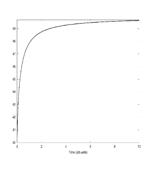
Figure 1 2.6 [ M − N λ / ( λ + μ ) ] < 0 delimited-[] 𝑀 𝑁 𝜆 𝜆 𝜇 0 \left[M-N\lambda/(\lambda+\mu)\right]<0 [ M − N λ / ( λ + μ ) ] > 0 delimited-[] 𝑀 𝑁 𝜆 𝜆 𝜇 0 \left[M-N\lambda/(\lambda+\mu)\right]>0 M = N λ / ( λ + μ ) 𝑀 𝑁 𝜆 𝜆 𝜇 M=N\lambda/(\lambda+\mu) 𝔼 𝒩 ν ( t ) = N λ / ( λ + μ ) 𝔼 superscript 𝒩 𝜈 𝑡 𝑁 𝜆 𝜆 𝜇 \mathbb{E}\,\mathcal{N}^{\nu}(t)=N\lambda/(\lambda+\mu)
Figure 1: The mean value of the fractional binomial process 𝔼 𝒩 ν ( t ) 𝔼 superscript 𝒩 𝜈 𝑡 \mathbb{E}\,\mathcal{N}^{\nu}(t) N = 100 𝑁 100 N=100 M = 40 𝑀 40 M=40 ν = 0.7 𝜈 0.7 \nu=0.7 ( λ , μ ) = ( 1 , 1 ) 𝜆 𝜇 1 1 (\lambda,\mu)=(1,1) ( λ , μ ) = ( 1 , 3 ) 𝜆 𝜇 1 3 (\lambda,\mu)=(1,3)
We now proceed to deriving the variance 𝕍 ar 𝒩 ν ( t ) 𝕍 ar superscript 𝒩 𝜈 𝑡 \mathbb{V}\text{ar}\,\mathcal{N}^{\nu}(t)
Theorem 3
For the fractional binomial process 𝒩 ν ( t ) superscript 𝒩 𝜈 𝑡 \mathcal{N}^{\nu}(t) t ≥ 0 𝑡 0 t\geq 0 ν ∈ ( 0 , 1 ] 𝜈 0 1 \nu\in(0,1]
𝕍 ar 𝕍 ar \displaystyle\mathbb{V}\text{ar} 𝒩 ν ( t ) superscript 𝒩 𝜈 𝑡 \displaystyle\,\mathcal{N}^{\nu}(t) (2.11)
= \displaystyle={} ( λ 2 N ( N − 1 ) ( λ + μ ) 2 − 2 λ M ( N − 1 ) λ + μ + M ( M − 1 ) ) E ν , 1 ( − 2 ( λ + μ ) t ν ) superscript 𝜆 2 𝑁 𝑁 1 superscript 𝜆 𝜇 2 2 𝜆 𝑀 𝑁 1 𝜆 𝜇 𝑀 𝑀 1 subscript 𝐸 𝜈 1
2 𝜆 𝜇 superscript 𝑡 𝜈 \displaystyle\left(\frac{\lambda^{2}N(N-1)}{(\lambda+\mu)^{2}}-\frac{2\lambda M(N-1)}{\lambda+\mu}+M(M-1)\right)E_{\nu,1}(-2(\lambda+\mu)t^{\nu})
+ ( 2 λ 2 N ( λ + μ ) 2 − λ λ + μ ( N + 2 M ) + M ) E ν , 1 ( − ( λ + μ ) t ν ) 2 superscript 𝜆 2 𝑁 superscript 𝜆 𝜇 2 𝜆 𝜆 𝜇 𝑁 2 𝑀 𝑀 subscript 𝐸 𝜈 1
𝜆 𝜇 superscript 𝑡 𝜈 \displaystyle+\left(\frac{2\lambda^{2}N}{(\lambda+\mu)^{2}}-\frac{\lambda}{\lambda+\mu}(N+2M)+M\right)E_{\nu,1}(-(\lambda+\mu)t^{\nu})
− ( M − N λ λ + μ ) 2 ( E ν , 1 ( − ( λ + μ ) t ν ) ) 2 + N λ μ ( λ + μ ) 2 . superscript 𝑀 𝑁 𝜆 𝜆 𝜇 2 superscript subscript 𝐸 𝜈 1
𝜆 𝜇 superscript 𝑡 𝜈 2 𝑁 𝜆 𝜇 superscript 𝜆 𝜇 2 \displaystyle-\left(M-N\frac{\lambda}{\lambda+\mu}\right)^{2}\left(E_{\nu,1}(-(\lambda+\mu)t^{\nu})\right)^{2}+\frac{N\lambda\mu}{(\lambda+\mu)^{2}}.
Proof
From ( 1.5 ), we have
∂ ν ∂ t ν ∂ 2 ∂ u 2 Q ν ( u , t ) = superscript 𝜈 superscript 𝑡 𝜈 superscript 2 superscript 𝑢 2 superscript 𝑄 𝜈 𝑢 𝑡 absent \displaystyle\frac{\partial^{\nu}}{\partial t^{\nu}}\frac{\partial^{2}}{\partial u^{2}}Q^{\nu}(u,t)={} − μ ∂ 2 ∂ u 2 Q ν ( u , t ) − μ ( ∂ 2 ∂ u 2 Q ν ( u , t ) + u ∂ 3 ∂ u 3 Q ν ( u , t ) ) 𝜇 superscript 2 superscript 𝑢 2 superscript 𝑄 𝜈 𝑢 𝑡 𝜇 superscript 2 superscript 𝑢 2 superscript 𝑄 𝜈 𝑢 𝑡 𝑢 superscript 3 superscript 𝑢 3 superscript 𝑄 𝜈 𝑢 𝑡 \displaystyle-\mu\frac{\partial^{2}}{\partial u^{2}}Q^{\nu}(u,t)-\mu\left(\frac{\partial^{2}}{\partial u^{2}}Q^{\nu}(u,t)+u\frac{\partial^{3}}{\partial u^{3}}Q^{\nu}(u,t)\right) (2.12)
− λ ( ( 1 − 2 u ) ∂ 2 ∂ u 2 Q ν ( u , t ) − 2 ∂ ∂ u Q ν ( u , t ) ) 𝜆 1 2 𝑢 superscript 2 superscript 𝑢 2 superscript 𝑄 𝜈 𝑢 𝑡 2 𝑢 superscript 𝑄 𝜈 𝑢 𝑡 \displaystyle-\lambda\left((1-2u)\frac{\partial^{2}}{\partial u^{2}}Q^{\nu}(u,t)-2\frac{\partial}{\partial u}Q^{\nu}(u,t)\right)
− λ ( ( 1 − 2 u ) ∂ 2 ∂ u 2 Q ν ( u , t ) + ( u − u 2 ) ∂ 3 ∂ u 3 Q ν ( u , t ) ) 𝜆 1 2 𝑢 superscript 2 superscript 𝑢 2 superscript 𝑄 𝜈 𝑢 𝑡 𝑢 superscript 𝑢 2 superscript 3 superscript 𝑢 3 superscript 𝑄 𝜈 𝑢 𝑡 \displaystyle-\lambda\left((1-2u)\frac{\partial^{2}}{\partial u^{2}}Q^{\nu}(u,t)+(u-u^{2})\frac{\partial^{3}}{\partial u^{3}}Q^{\nu}(u,t)\right)
− λ N ∂ ∂ u Q ν ( u , t ) − λ N ( ∂ ∂ u Q ν ( u , t ) + u ∂ 2 ∂ u 2 Q ν ( u , t ) ) . 𝜆 𝑁 𝑢 superscript 𝑄 𝜈 𝑢 𝑡 𝜆 𝑁 𝑢 superscript 𝑄 𝜈 𝑢 𝑡 𝑢 superscript 2 superscript 𝑢 2 superscript 𝑄 𝜈 𝑢 𝑡 \displaystyle-\lambda N\frac{\partial}{\partial u}Q^{\nu}(u,t)-\lambda N\left(\frac{\partial}{\partial u}Q^{\nu}(u,t)+u\frac{\partial^{2}}{\partial u^{2}}Q^{\nu}(u,t)\right).
Recalling ( 2.7 ) and the equality
∂ 2 ∂ u 2 Q ν ( u , t ) | u = 0 = 𝔼 ( 𝒩 ν ( t ) ( 𝒩 ν ( t ) − 1 ) ) = H ν ( t ) , evaluated-at superscript 2 superscript 𝑢 2 superscript 𝑄 𝜈 𝑢 𝑡 𝑢 0 𝔼 superscript 𝒩 𝜈 𝑡 superscript 𝒩 𝜈 𝑡 1 superscript 𝐻 𝜈 𝑡 \displaystyle\left.\frac{\partial^{2}}{\partial u^{2}}Q^{\nu}(u,t)\right|_{u=0}=\mathbb{E}\left(\mathcal{N}^{\nu}(t)(\mathcal{N}^{\nu}(t)-1)\right)=H^{\nu}(t), (2.13)
we obtain
d ν d t ν H ν ( t ) superscript d 𝜈 d superscript 𝑡 𝜈 superscript 𝐻 𝜈 𝑡 \displaystyle\frac{\mathrm{d}^{\nu}}{\mathrm{d}t^{\nu}}H^{\nu}(t) = − 2 μ H ν ( t ) − 2 λ H ν ( t ) − 2 λ 𝔼 𝒩 ν ( t ) + 2 λ N 𝔼 𝒩 ν ( t ) absent 2 𝜇 superscript 𝐻 𝜈 𝑡 2 𝜆 superscript 𝐻 𝜈 𝑡 2 𝜆 𝔼 superscript 𝒩 𝜈 𝑡 2 𝜆 𝑁 𝔼 superscript 𝒩 𝜈 𝑡 \displaystyle=-2\mu H^{\nu}(t)-2\lambda H^{\nu}(t)-2\lambda\mathbb{E}\,\mathcal{N}^{\nu}(t)+2\lambda N\mathbb{E}\,\mathcal{N}^{\nu}(t) (2.14)
= − 2 ( λ + μ ) H ν ( t ) + 2 λ ( N − 1 ) 𝔼 𝒩 ν ( t ) . absent 2 𝜆 𝜇 superscript 𝐻 𝜈 𝑡 2 𝜆 𝑁 1 𝔼 superscript 𝒩 𝜈 𝑡 \displaystyle=-2(\lambda+\mu)H^{\nu}(t)+2\lambda(N-1)\mathbb{E}\,\mathcal{N}^{\nu}(t).
By substituting ( 2.6 ) into ( 2.14 ), we arrive at the Cauchy problem
{ d ν d t ν H ν ( t ) = − 2 ( λ + μ ) H ν ( t ) + 2 λ ( N − 1 ) ( M − N λ λ + μ ) E ν , 1 ( − ( λ + μ ) t ν ) + 2 λ 2 N ( N − 1 ) 1 λ + μ H ν ( 0 ) = M ( M − 1 ) , cases superscript d 𝜈 d superscript 𝑡 𝜈 superscript 𝐻 𝜈 𝑡 2 𝜆 𝜇 superscript 𝐻 𝜈 𝑡 2 𝜆 𝑁 1 𝑀 𝑁 𝜆 𝜆 𝜇 subscript 𝐸 𝜈 1
𝜆 𝜇 superscript 𝑡 𝜈 otherwise 2 superscript 𝜆 2 𝑁 𝑁 1 1 𝜆 𝜇 otherwise superscript 𝐻 𝜈 0 𝑀 𝑀 1 otherwise \displaystyle\begin{cases}\frac{\mathrm{d}^{\nu}}{\mathrm{d}t^{\nu}}H^{\nu}(t)=-2(\lambda+\mu)H^{\nu}(t)+2\lambda(N-1)\left(M-N\frac{\lambda}{\lambda+\mu}\right)E_{\nu,1}\left(-(\lambda+\mu)t^{\nu}\right)\\
\qquad\qquad\qquad+2\lambda^{2}N(N-1)\frac{1}{\lambda+\mu}\\
H^{\nu}(0)=M(M-1),\end{cases} (2.15)
that can be solved using the Laplace transform H ~ ν ( z ) = ∫ 0 ∞ e − z t H ν ( t ) d t superscript ~ 𝐻 𝜈 𝑧 superscript subscript 0 superscript 𝑒 𝑧 𝑡 superscript 𝐻 𝜈 𝑡 differential-d 𝑡 \widetilde{H}^{\nu}(z)=\int_{0}^{\infty}e^{-zt}H^{\nu}(t)\,\mathrm{d}t as follows:
z ν H ~ ν ( z ) superscript 𝑧 𝜈 superscript ~ 𝐻 𝜈 𝑧 \displaystyle z^{\nu}\widetilde{H}^{\nu}(z) − z ν − 1 M ( M − 1 ) superscript 𝑧 𝜈 1 𝑀 𝑀 1 \displaystyle-z^{\nu-1}M(M-1) (2.16)
= \displaystyle={} − 2 ( λ + μ ) H ~ ν ( z ) + 2 λ ( N − 1 ) ( M − N λ λ + μ ) z ν − 1 z ν + ( λ + μ ) 2 𝜆 𝜇 superscript ~ 𝐻 𝜈 𝑧 2 𝜆 𝑁 1 𝑀 𝑁 𝜆 𝜆 𝜇 superscript 𝑧 𝜈 1 superscript 𝑧 𝜈 𝜆 𝜇 \displaystyle-2(\lambda+\mu)\widetilde{H}^{\nu}(z)+2\lambda(N-1)\left(M-N\frac{\lambda}{\lambda+\mu}\right)\frac{z^{\nu-1}}{z^{\nu}+(\lambda+\mu)}
+ 1 z 2 λ 2 N ( N − 1 ) 1 λ + μ . 1 𝑧 2 superscript 𝜆 2 𝑁 𝑁 1 1 𝜆 𝜇 \displaystyle+\frac{1}{z}2\lambda^{2}N(N-1)\frac{1}{\lambda+\mu}.
The Laplace transform then reads
H ~ ν ( z ) = superscript ~ 𝐻 𝜈 𝑧 absent \displaystyle\widetilde{H}^{\nu}(z)={} M ( M − 1 ) z ν − 1 z ν + 2 ( λ + μ ) 𝑀 𝑀 1 superscript 𝑧 𝜈 1 superscript 𝑧 𝜈 2 𝜆 𝜇 \displaystyle M(M-1)\frac{z^{\nu-1}}{z^{\nu}+2(\lambda+\mu)} (2.17)
+ 2 λ ( N − 1 ) ( M − N λ λ + μ ) z ν − 1 ( z ν + ( λ + μ ) ) ( z ν + 2 ( λ + μ ) ) 2 𝜆 𝑁 1 𝑀 𝑁 𝜆 𝜆 𝜇 superscript 𝑧 𝜈 1 superscript 𝑧 𝜈 𝜆 𝜇 superscript 𝑧 𝜈 2 𝜆 𝜇 \displaystyle+2\lambda(N-1)\left(M-N\frac{\lambda}{\lambda+\mu}\right)\frac{z^{\nu-1}}{(z^{\nu}+(\lambda+\mu))(z^{\nu}+2(\lambda+\mu))}
+ 2 λ 2 N ( N − 1 ) 1 λ + μ ⋅ z − 1 z ν + 2 ( λ + μ ) ⋅ 2 superscript 𝜆 2 𝑁 𝑁 1 1 𝜆 𝜇 superscript 𝑧 1 superscript 𝑧 𝜈 2 𝜆 𝜇 \displaystyle+2\lambda^{2}N(N-1)\frac{1}{\lambda+\mu}\cdot\frac{z^{-1}}{z^{\nu}+2(\lambda+\mu)}
= \displaystyle={} M ( M − 1 ) z ν − 1 z ν + 2 ( λ + μ ) 𝑀 𝑀 1 superscript 𝑧 𝜈 1 superscript 𝑧 𝜈 2 𝜆 𝜇 \displaystyle M(M-1)\frac{z^{\nu-1}}{z^{\nu}+2(\lambda+\mu)}
+ 2 λ ( N − 1 ) λ + μ ( M − N λ λ + μ ) ( z ν − 1 z ν + ( λ + μ ) − z ν − 1 z ν + 2 ( λ + μ ) ) 2 𝜆 𝑁 1 𝜆 𝜇 𝑀 𝑁 𝜆 𝜆 𝜇 superscript 𝑧 𝜈 1 superscript 𝑧 𝜈 𝜆 𝜇 superscript 𝑧 𝜈 1 superscript 𝑧 𝜈 2 𝜆 𝜇 \displaystyle+\frac{2\lambda(N-1)}{\lambda+\mu}\left(M-N\frac{\lambda}{\lambda+\mu}\right)\left(\frac{z^{\nu-1}}{z^{\nu}+(\lambda+\mu)}-\frac{z^{\nu-1}}{z^{\nu}+2(\lambda+\mu)}\right)
+ 2 λ 2 N ( N − 1 ) 1 λ + μ ⋅ z − 1 z ν + 2 ( λ + μ ) . ⋅ 2 superscript 𝜆 2 𝑁 𝑁 1 1 𝜆 𝜇 superscript 𝑧 1 superscript 𝑧 𝜈 2 𝜆 𝜇 \displaystyle+2\lambda^{2}N(N-1)\frac{1}{\lambda+\mu}\cdot\frac{z^{-1}}{z^{\nu}+2(\lambda+\mu)}.
Equation ( 2.17 ) then implies that
H ν superscript 𝐻 𝜈 \displaystyle H^{\nu} ( t ) 𝑡 \displaystyle(t) (2.18)
= \displaystyle={} M ( M − 1 ) E ν , 1 ( − 2 ( λ + μ ) t ν ) 𝑀 𝑀 1 subscript 𝐸 𝜈 1
2 𝜆 𝜇 superscript 𝑡 𝜈 \displaystyle M(M-1)E_{\nu,1}\left(-2(\lambda+\mu)t^{\nu}\right)
+ 2 λ ( N − 1 ) λ + μ ( M − N λ λ + μ ) ( E ν , 1 ( − ( λ + μ ) t ν ) − E ν , 1 ( − 2 ( λ + μ ) t ν ) ) 2 𝜆 𝑁 1 𝜆 𝜇 𝑀 𝑁 𝜆 𝜆 𝜇 subscript 𝐸 𝜈 1
𝜆 𝜇 superscript 𝑡 𝜈 subscript 𝐸 𝜈 1
2 𝜆 𝜇 superscript 𝑡 𝜈 \displaystyle+\frac{2\lambda(N-1)}{\lambda+\mu}\left(M-N\frac{\lambda}{\lambda+\mu}\right)\left(E_{\nu,1}(-(\lambda+\mu)t^{\nu})-E_{\nu,1}(-2(\lambda+\mu)t^{\nu})\right)
+ 2 λ 2 N ( N − 1 ) 1 λ + μ t ν E ν , ν + 1 ( − 2 ( λ + μ ) t ν ) . 2 superscript 𝜆 2 𝑁 𝑁 1 1 𝜆 𝜇 superscript 𝑡 𝜈 subscript 𝐸 𝜈 𝜈 1
2 𝜆 𝜇 superscript 𝑡 𝜈 \displaystyle+2\lambda^{2}N(N-1)\frac{1}{\lambda+\mu}t^{\nu}E_{\nu,\nu+1}\left(-2(\lambda+\mu)t^{\nu}\right).
Considering that t ν E ν , ν + 1 ( a t ν ) = a − 1 ( E ν , 1 ( a t ν ) − 1 ) superscript 𝑡 𝜈 subscript 𝐸 𝜈 𝜈 1
𝑎 superscript 𝑡 𝜈 superscript 𝑎 1 subscript 𝐸 𝜈 1
𝑎 superscript 𝑡 𝜈 1 t^{\nu}E_{\nu,\nu+1}(at^{\nu})=a^{-1}(E_{\nu,1}(at^{\nu})-1) , we obtain
H ν ( t ) = superscript 𝐻 𝜈 𝑡 absent \displaystyle H^{\nu}(t)={} M ( M − 1 ) E ν , 1 ( − 2 ( λ + μ ) t ν ) 𝑀 𝑀 1 subscript 𝐸 𝜈 1
2 𝜆 𝜇 superscript 𝑡 𝜈 \displaystyle M(M-1)E_{\nu,1}\left(-2(\lambda+\mu)t^{\nu}\right) (2.19)
+ 2 λ ( N − 1 ) λ + μ ( M − N λ λ + μ ) E ν , 1 ( − ( λ + μ ) t ν ) 2 𝜆 𝑁 1 𝜆 𝜇 𝑀 𝑁 𝜆 𝜆 𝜇 subscript 𝐸 𝜈 1
𝜆 𝜇 superscript 𝑡 𝜈 \displaystyle+\frac{2\lambda(N-1)}{\lambda+\mu}\left(M-N\frac{\lambda}{\lambda+\mu}\right)E_{\nu,1}(-(\lambda+\mu)t^{\nu})
− 2 λ ( N − 1 ) λ + μ ( M − N λ λ + μ ) E ν , 1 ( − 2 ( λ + μ ) t ν ) 2 𝜆 𝑁 1 𝜆 𝜇 𝑀 𝑁 𝜆 𝜆 𝜇 subscript 𝐸 𝜈 1
2 𝜆 𝜇 superscript 𝑡 𝜈 \displaystyle-\frac{2\lambda(N-1)}{\lambda+\mu}\left(M-N\frac{\lambda}{\lambda+\mu}\right)E_{\nu,1}(-2(\lambda+\mu)t^{\nu})
− λ 2 ( λ + μ ) 2 N ( N − 1 ) E ν , 1 ( − 2 ( λ + μ ) t ν ) + λ 2 ( λ + μ ) 2 N ( N − 1 ) superscript 𝜆 2 superscript 𝜆 𝜇 2 𝑁 𝑁 1 subscript 𝐸 𝜈 1
2 𝜆 𝜇 superscript 𝑡 𝜈 superscript 𝜆 2 superscript 𝜆 𝜇 2 𝑁 𝑁 1 \displaystyle-\frac{\lambda^{2}}{(\lambda+\mu)^{2}}N(N-1)E_{\nu,1}(-2(\lambda+\mu)t^{\nu})+\frac{\lambda^{2}}{(\lambda+\mu)^{2}}N(N-1)
= \displaystyle={} M ( M − 1 ) E ν , 1 ( − 2 ( λ + μ ) t ν ) 𝑀 𝑀 1 subscript 𝐸 𝜈 1
2 𝜆 𝜇 superscript 𝑡 𝜈 \displaystyle M(M-1)E_{\nu,1}\left(-2(\lambda+\mu)t^{\nu}\right)
+ 2 λ M ( N − 1 ) λ + μ E ν , 1 ( − ( λ + μ ) t ν ) 2 𝜆 𝑀 𝑁 1 𝜆 𝜇 subscript 𝐸 𝜈 1
𝜆 𝜇 superscript 𝑡 𝜈 \displaystyle+\frac{2\lambda M(N-1)}{\lambda+\mu}E_{\nu,1}(-(\lambda+\mu)t^{\nu})
− 2 λ 2 N ( N − 1 ) ( λ + μ ) 2 E ν , 1 ( − ( λ + μ ) t ν ) 2 superscript 𝜆 2 𝑁 𝑁 1 superscript 𝜆 𝜇 2 subscript 𝐸 𝜈 1
𝜆 𝜇 superscript 𝑡 𝜈 \displaystyle-\frac{2\lambda^{2}N(N-1)}{(\lambda+\mu)^{2}}E_{\nu,1}(-(\lambda+\mu)t^{\nu})
− 2 λ M ( N − 1 ) λ + μ E ν , 1 ( − 2 ( λ + μ ) t ν ) 2 𝜆 𝑀 𝑁 1 𝜆 𝜇 subscript 𝐸 𝜈 1
2 𝜆 𝜇 superscript 𝑡 𝜈 \displaystyle-\frac{2\lambda M(N-1)}{\lambda+\mu}E_{\nu,1}(-2(\lambda+\mu)t^{\nu})
+ 2 λ 2 N ( N − 1 ) ( λ + μ ) 2 E ν , 1 ( − 2 ( λ + μ ) t ν ) 2 superscript 𝜆 2 𝑁 𝑁 1 superscript 𝜆 𝜇 2 subscript 𝐸 𝜈 1
2 𝜆 𝜇 superscript 𝑡 𝜈 \displaystyle+\frac{2\lambda^{2}N(N-1)}{(\lambda+\mu)^{2}}E_{\nu,1}(-2(\lambda+\mu)t^{\nu})
− λ 2 N ( N − 1 ) ( λ + μ ) 2 E ν , 1 ( − 2 ( λ + μ ) t ν ) + λ 2 N ( N − 1 ) ( λ + μ ) 2 superscript 𝜆 2 𝑁 𝑁 1 superscript 𝜆 𝜇 2 subscript 𝐸 𝜈 1
2 𝜆 𝜇 superscript 𝑡 𝜈 superscript 𝜆 2 𝑁 𝑁 1 superscript 𝜆 𝜇 2 \displaystyle-\frac{\lambda^{2}N(N-1)}{(\lambda+\mu)^{2}}E_{\nu,1}(-2(\lambda+\mu)t^{\nu})+\frac{\lambda^{2}N(N-1)}{(\lambda+\mu)^{2}}
= \displaystyle={} λ 2 N ( N − 1 ) ( λ + μ ) 2 superscript 𝜆 2 𝑁 𝑁 1 superscript 𝜆 𝜇 2 \displaystyle\frac{\lambda^{2}N(N-1)}{(\lambda+\mu)^{2}}
+ E ν , 1 ( − 2 ( λ + μ ) t ν ) ( λ 2 N ( N − 1 ) ( λ + μ ) 2 − 2 λ M ( N − 1 ) λ + μ + M ( M − 1 ) ) subscript 𝐸 𝜈 1
2 𝜆 𝜇 superscript 𝑡 𝜈 superscript 𝜆 2 𝑁 𝑁 1 superscript 𝜆 𝜇 2 2 𝜆 𝑀 𝑁 1 𝜆 𝜇 𝑀 𝑀 1 \displaystyle+E_{\nu,1}(-2(\lambda+\mu)t^{\nu})\left(\frac{\lambda^{2}N(N-1)}{(\lambda+\mu)^{2}}-\frac{2\lambda M(N-1)}{\lambda+\mu}+M(M-1)\right)
− E ν , 1 ( − ( λ + μ ) t ν ) ( 2 λ 2 N ( N − 1 ) ( λ + μ ) 2 − 2 λ M ( N − 1 ) λ + μ ) . subscript 𝐸 𝜈 1
𝜆 𝜇 superscript 𝑡 𝜈 2 superscript 𝜆 2 𝑁 𝑁 1 superscript 𝜆 𝜇 2 2 𝜆 𝑀 𝑁 1 𝜆 𝜇 \displaystyle-E_{\nu,1}(-(\lambda+\mu)t^{\nu})\left(\frac{2\lambda^{2}N(N-1)}{(\lambda+\mu)^{2}}-\frac{2\lambda M(N-1)}{\lambda+\mu}\right).
The variance can thus be written as
𝕍 ar 𝕍 ar \displaystyle\mathbb{V}\text{ar} 𝒩 ν ( t ) superscript 𝒩 𝜈 𝑡 \displaystyle\,\mathcal{N}^{\nu}(t) (2.20)
= \displaystyle={} H ν ( t ) + 𝔼 𝒩 ν ( t ) − ( 𝔼 𝒩 ν ( t ) ) 2 superscript 𝐻 𝜈 𝑡 𝔼 superscript 𝒩 𝜈 𝑡 superscript 𝔼 superscript 𝒩 𝜈 𝑡 2 \displaystyle H^{\nu}(t)+\mathbb{E}\,\mathcal{N}^{\nu}(t)-(\mathbb{E}\,\mathcal{N}^{\nu}(t))^{2}
= \displaystyle={} H ν ( t ) + ( M − N λ λ + μ ) E ν , 1 ( − ( λ + μ ) t ν ) superscript 𝐻 𝜈 𝑡 𝑀 𝑁 𝜆 𝜆 𝜇 subscript 𝐸 𝜈 1
𝜆 𝜇 superscript 𝑡 𝜈 \displaystyle H^{\nu}(t)+\left(M-N\frac{\lambda}{\lambda+\mu}\right)E_{\nu,1}(-(\lambda+\mu)t^{\nu})
+ N λ λ + μ − ( M − λ λ + μ ) 2 ( E ν , 1 ( − ( λ + μ ) t ν ) ) 2 𝑁 𝜆 𝜆 𝜇 superscript 𝑀 𝜆 𝜆 𝜇 2 superscript subscript 𝐸 𝜈 1
𝜆 𝜇 superscript 𝑡 𝜈 2 \displaystyle+N\frac{\lambda}{\lambda+\mu}-\left(M-\frac{\lambda}{\lambda+\mu}\right)^{2}\left(E_{\nu,1}(-(\lambda+\mu)t^{\nu})\right)^{2}
− N 2 λ 2 ( λ + μ ) 2 − 2 N λ λ + μ ( M − N λ λ + μ ) E ν , 1 ( − ( λ + μ ) t ν ) superscript 𝑁 2 superscript 𝜆 2 superscript 𝜆 𝜇 2 2 𝑁 𝜆 𝜆 𝜇 𝑀 𝑁 𝜆 𝜆 𝜇 subscript 𝐸 𝜈 1
𝜆 𝜇 superscript 𝑡 𝜈 \displaystyle-N^{2}\frac{\lambda^{2}}{(\lambda+\mu)^{2}}-2\frac{N\lambda}{\lambda+\mu}\left(M-N\frac{\lambda}{\lambda+\mu}\right)E_{\nu,1}(-(\lambda+\mu)t^{\nu})
= \displaystyle={} ( λ 2 N ( N − 1 ) ( λ + μ ) 2 − 2 λ M ( N − 1 ) λ + μ + M ( M − 1 ) ) E ν , 1 ( − 2 ( λ + μ ) t ν ) superscript 𝜆 2 𝑁 𝑁 1 superscript 𝜆 𝜇 2 2 𝜆 𝑀 𝑁 1 𝜆 𝜇 𝑀 𝑀 1 subscript 𝐸 𝜈 1
2 𝜆 𝜇 superscript 𝑡 𝜈 \displaystyle\left(\frac{\lambda^{2}N(N-1)}{(\lambda+\mu)^{2}}-\frac{2\lambda M(N-1)}{\lambda+\mu}+M(M-1)\right)E_{\nu,1}(-2(\lambda+\mu)t^{\nu})
+ ( 2 λ 2 N ( λ + μ ) 2 − λ λ + μ ( N + 2 M ) + M ) E ν , 1 ( − ( λ + μ ) t ν ) 2 superscript 𝜆 2 𝑁 superscript 𝜆 𝜇 2 𝜆 𝜆 𝜇 𝑁 2 𝑀 𝑀 subscript 𝐸 𝜈 1
𝜆 𝜇 superscript 𝑡 𝜈 \displaystyle+\left(\frac{2\lambda^{2}N}{(\lambda+\mu)^{2}}-\frac{\lambda}{\lambda+\mu}(N+2M)+M\right)E_{\nu,1}(-(\lambda+\mu)t^{\nu})
− ( M − N λ λ + μ ) 2 ( E ν , 1 ( − ( λ + μ ) t ν ) ) 2 + N λ μ ( λ + μ ) 2 . superscript 𝑀 𝑁 𝜆 𝜆 𝜇 2 superscript subscript 𝐸 𝜈 1
𝜆 𝜇 superscript 𝑡 𝜈 2 𝑁 𝜆 𝜇 superscript 𝜆 𝜇 2 \displaystyle-\left(M-N\frac{\lambda}{\lambda+\mu}\right)^{2}\left(E_{\nu,1}(-(\lambda+\mu)t^{\nu})\right)^{2}+\frac{N\lambda\mu}{(\lambda+\mu)^{2}}.
Exploiting Theorem 1 p 0 ν ( t ) = Pr { 𝒩 ν ( t ) = 0 | 𝒩 ν ( 0 ) = M } superscript subscript 𝑝 0 𝜈 𝑡 Pr conditional-set superscript 𝒩 𝜈 𝑡 0 superscript 𝒩 𝜈 0 𝑀 p_{0}^{\nu}(t)=\text{Pr}\{\mathcal{N}^{\nu}(t)=0|\mathcal{N}^{\nu}(0)=M\}
Theorem 4
The extinction probability p 0 ν ( t ) = Pr { 𝒩 ν ( t ) = 0 | 𝒩 ν ( 0 ) = M } superscript subscript 𝑝 0 𝜈 𝑡 Pr conditional-set superscript 𝒩 𝜈 𝑡 0 superscript 𝒩 𝜈 0 𝑀 p_{0}^{\nu}(t)=\text{Pr}\{\mathcal{N}^{\nu}(t)=0|\mathcal{N}^{\nu}(0)=M\} 𝒩 ν ( t ) superscript 𝒩 𝜈 𝑡 \mathcal{N}^{\nu}(t) t ≥ 0 𝑡 0 t\geq 0
p 0 ν ( t ) = superscript subscript 𝑝 0 𝜈 𝑡 absent \displaystyle p_{0}^{\nu}(t)={} ( μ λ + μ ) N ∑ r = 0 N − M ( N − M r ) ( λ μ ) r superscript 𝜇 𝜆 𝜇 𝑁 superscript subscript 𝑟 0 𝑁 𝑀 binomial 𝑁 𝑀 𝑟 superscript 𝜆 𝜇 𝑟 \displaystyle\left(\frac{\mu}{\lambda+\mu}\right)^{N}\sum_{r=0}^{N-M}\binom{N-M}{r}\left(\frac{\lambda}{\mu}\right)^{r} (2.21)
× ∑ h = 0 M ( M h ) ( − 1 ) h E ν , 1 ( − ( r + h ) ( λ + μ ) t ν ) . \displaystyle\times\sum_{h=0}^{M}\binom{M}{h}(-1)^{h}E_{\nu,1}(-(r+h)(\lambda+\mu)t^{\nu}).
Proof
It is known ( Jakeman, 1990 ) that the generating function Q ( u , t ) = ∑ n = 0 N ( 1 − u ) n p n ( t ) 𝑄 𝑢 𝑡 superscript subscript 𝑛 0 𝑁 superscript 1 𝑢 𝑛 subscript 𝑝 𝑛 𝑡 Q(u,t)=\sum_{n=0}^{N}(1-u)^{n}p_{n}(t)
for the classical binomial process can be written as
Q ( u , t ) = 𝑄 𝑢 𝑡 absent \displaystyle Q(u,t)={} [ 1 − ( 1 − e − ( μ + λ ) t ) λ λ + μ u ] N − M superscript delimited-[] 1 1 superscript 𝑒 𝜇 𝜆 𝑡 𝜆 𝜆 𝜇 𝑢 𝑁 𝑀 \displaystyle\left[1-\left(1-e^{-(\mu+\lambda)t}\right)\frac{\lambda}{\lambda+\mu}u\right]^{N-M} (2.22)
× [ 1 − ( ( 1 − e − ( μ + λ ) t ) λ λ + μ + e − ( μ + λ ) t ) u ] M . absent superscript delimited-[] 1 1 superscript 𝑒 𝜇 𝜆 𝑡 𝜆 𝜆 𝜇 superscript 𝑒 𝜇 𝜆 𝑡 𝑢 𝑀 \displaystyle\times\left[1-\left(\left(1-e^{-(\mu+\lambda)t}\right)\frac{\lambda}{\lambda+\mu}+e^{-(\mu+\lambda)t}\right)u\right]^{M}.
This suggests that the extinction probability for the classical case can be written as
p 0 ( t ) = subscript 𝑝 0 𝑡 absent \displaystyle p_{0}(t)={} [ 1 − λ λ + μ + λ λ + μ e − ( μ + λ ) t ] N − M superscript delimited-[] 1 𝜆 𝜆 𝜇 𝜆 𝜆 𝜇 superscript 𝑒 𝜇 𝜆 𝑡 𝑁 𝑀 \displaystyle\left[1-\frac{\lambda}{\lambda+\mu}+\frac{\lambda}{\lambda+\mu}e^{-(\mu+\lambda)t}\right]^{N-M} (2.23)
× [ 1 − ( λ λ + μ − e − ( μ + λ ) t λ λ + μ + e − ( μ + λ ) t ) ] M absent superscript delimited-[] 1 𝜆 𝜆 𝜇 superscript 𝑒 𝜇 𝜆 𝑡 𝜆 𝜆 𝜇 superscript 𝑒 𝜇 𝜆 𝑡 𝑀 \displaystyle\times\left[1-\left(\frac{\lambda}{\lambda+\mu}-e^{-(\mu+\lambda)t}\frac{\lambda}{\lambda+\mu}+e^{-(\mu+\lambda)t}\right)\right]^{M}
= \displaystyle={} [ μ λ + μ + λ λ + μ e − ( μ + λ ) t ] N − M [ μ λ + μ − μ λ + μ e − ( μ + λ ) t ] M superscript delimited-[] 𝜇 𝜆 𝜇 𝜆 𝜆 𝜇 superscript 𝑒 𝜇 𝜆 𝑡 𝑁 𝑀 superscript delimited-[] 𝜇 𝜆 𝜇 𝜇 𝜆 𝜇 superscript 𝑒 𝜇 𝜆 𝑡 𝑀 \displaystyle\left[\frac{\mu}{\lambda+\mu}+\frac{\lambda}{\lambda+\mu}e^{-(\mu+\lambda)t}\right]^{N-M}\left[\frac{\mu}{\lambda+\mu}-\frac{\mu}{\lambda+\mu}e^{-(\mu+\lambda)t}\right]^{M}
= \displaystyle={} ( 1 λ + μ ) N μ M ( μ + λ e − ( λ + μ ) t ) N − M ( 1 − e − ( λ + μ ) t ) M superscript 1 𝜆 𝜇 𝑁 superscript 𝜇 𝑀 superscript 𝜇 𝜆 superscript 𝑒 𝜆 𝜇 𝑡 𝑁 𝑀 superscript 1 superscript 𝑒 𝜆 𝜇 𝑡 𝑀 \displaystyle\left(\frac{1}{\lambda+\mu}\right)^{N}\mu^{M}\left(\mu+\lambda e^{-(\lambda+\mu)t}\right)^{N-M}\left(1-e^{-(\lambda+\mu)t}\right)^{M}
= \displaystyle={} ( μ λ + μ ) N ( 1 + λ μ e − ( λ + μ ) t ) N − M ( 1 − e − ( λ + μ ) t ) M superscript 𝜇 𝜆 𝜇 𝑁 superscript 1 𝜆 𝜇 superscript 𝑒 𝜆 𝜇 𝑡 𝑁 𝑀 superscript 1 superscript 𝑒 𝜆 𝜇 𝑡 𝑀 \displaystyle\left(\frac{\mu}{\lambda+\mu}\right)^{N}\left(1+\frac{\lambda}{\mu}e^{-(\lambda+\mu)t}\right)^{N-M}\left(1-e^{-(\lambda+\mu)t}\right)^{M}
= \displaystyle={} ( μ λ + μ ) N ∑ r = 0 N − M ( N − M r ) ( λ μ ) r e − r ( λ + μ ) t superscript 𝜇 𝜆 𝜇 𝑁 superscript subscript 𝑟 0 𝑁 𝑀 binomial 𝑁 𝑀 𝑟 superscript 𝜆 𝜇 𝑟 superscript 𝑒 𝑟 𝜆 𝜇 𝑡 \displaystyle\left(\frac{\mu}{\lambda+\mu}\right)^{N}\sum_{r=0}^{N-M}\binom{N-M}{r}\left(\frac{\lambda}{\mu}\right)^{r}e^{-r(\lambda+\mu)t}
× ∑ h = 0 M ( M h ) ( − 1 ) h e − h ( λ + μ ) t \displaystyle\times\sum_{h=0}^{M}\binom{M}{h}(-1)^{h}e^{-h(\lambda+\mu)t}
= \displaystyle={} ( μ λ + μ ) N ∑ r = 0 N − M ( N − M r ) ( λ μ ) r ∑ h = 0 M ( M h ) ( − 1 ) h e − ( r + h ) ( λ + μ ) t . superscript 𝜇 𝜆 𝜇 𝑁 superscript subscript 𝑟 0 𝑁 𝑀 binomial 𝑁 𝑀 𝑟 superscript 𝜆 𝜇 𝑟 superscript subscript ℎ 0 𝑀 binomial 𝑀 ℎ superscript 1 ℎ superscript 𝑒 𝑟 ℎ 𝜆 𝜇 𝑡 \displaystyle\left(\frac{\mu}{\lambda+\mu}\right)^{N}\sum_{r=0}^{N-M}\binom{N-M}{r}\left(\frac{\lambda}{\mu}\right)^{r}\sum_{h=0}^{M}\binom{M}{h}(-1)^{h}e^{-(r+h)(\lambda+\mu)t}.
Using Theorem 1 , we now obtain
p 0 ν ( t ) = superscript subscript 𝑝 0 𝜈 𝑡 absent \displaystyle p_{0}^{\nu}(t)={} ∫ 0 ∞ p 0 ( s ) h ( s , t ) d s superscript subscript 0 subscript 𝑝 0 𝑠 ℎ 𝑠 𝑡 differential-d 𝑠 \displaystyle\int_{0}^{\infty}p_{0}(s)h(s,t)\mathrm{d}s (2.24)
= \displaystyle={} ( μ λ + μ ) N ∑ r = 0 N − M ( N − M r ) ( λ μ ) r superscript 𝜇 𝜆 𝜇 𝑁 superscript subscript 𝑟 0 𝑁 𝑀 binomial 𝑁 𝑀 𝑟 superscript 𝜆 𝜇 𝑟 \displaystyle\left(\frac{\mu}{\lambda+\mu}\right)^{N}\sum_{r=0}^{N-M}\binom{N-M}{r}\left(\frac{\lambda}{\mu}\right)^{r}
× ∑ h = 0 M ( M h ) ( − 1 ) h ∫ 0 ∞ e − ( r + h ) ( λ + μ ) s q ( s , t ) d s \displaystyle\times\sum_{h=0}^{M}\binom{M}{h}(-1)^{h}\int_{0}^{\infty}e^{-(r+h)(\lambda+\mu)s}q(s,t)\mathrm{d}s
= \displaystyle={} ( μ λ + μ ) N ∑ r = 0 N − M ( N − M r ) ( λ μ ) r superscript 𝜇 𝜆 𝜇 𝑁 superscript subscript 𝑟 0 𝑁 𝑀 binomial 𝑁 𝑀 𝑟 superscript 𝜆 𝜇 𝑟 \displaystyle\left(\frac{\mu}{\lambda+\mu}\right)^{N}\sum_{r=0}^{N-M}\binom{N-M}{r}\left(\frac{\lambda}{\mu}\right)^{r}
× ∑ h = 0 M ( M h ) ( − 1 ) h E ν , 1 ( − ( r + h ) ( λ + μ ) t ν ) . \displaystyle\times\sum_{h=0}^{M}\binom{M}{h}(-1)^{h}E_{\nu,1}(-(r+h)(\lambda+\mu)t^{\nu}).
Theorem 5
The state probabilities p n ν ( t ) = Pr { 𝒩 ν ( t ) = n | 𝒩 ν ( 0 ) = M } superscript subscript 𝑝 𝑛 𝜈 𝑡 Pr conditional-set superscript 𝒩 𝜈 𝑡 𝑛 superscript 𝒩 𝜈 0 𝑀 p_{n}^{\nu}(t)=\text{Pr}\{\mathcal{N}^{\nu}(t)=n|\mathcal{N}^{\nu}(0)=M\} λ > 0 𝜆 0 \lambda>0 μ > 0 𝜇 0 \mu>0
p n ν ( t ) = { ∑ r = 0 n g n , r ν ( t ) , 0 ≤ n < min ( M , N − M ) , ∑ r = 0 N − M g n , r ν ( t ) , N − M ≤ n < M , M > N − M , ∑ r = n − M n g n , r ν ( t ) , M ≤ n < N − M , M < N − M , ∑ r = n − M N − M g n , r ν ( t ) , max ( M , N − M ) ≤ n ≤ N , superscript subscript 𝑝 𝑛 𝜈 𝑡 cases superscript subscript 𝑟 0 𝑛 superscript subscript 𝑔 𝑛 𝑟
𝜈 𝑡 0 𝑛 𝑀 𝑁 𝑀 superscript subscript 𝑟 0 𝑁 𝑀 superscript subscript 𝑔 𝑛 𝑟
𝜈 𝑡 formulae-sequence 𝑁 𝑀 𝑛 𝑀 𝑀 𝑁 𝑀 superscript subscript 𝑟 𝑛 𝑀 𝑛 superscript subscript 𝑔 𝑛 𝑟
𝜈 𝑡 formulae-sequence 𝑀 𝑛 𝑁 𝑀 𝑀 𝑁 𝑀 superscript subscript 𝑟 𝑛 𝑀 𝑁 𝑀 superscript subscript 𝑔 𝑛 𝑟
𝜈 𝑡 𝑀 𝑁 𝑀 𝑛 𝑁 \displaystyle p_{n}^{\nu}(t)=\begin{cases}\sum_{r=0}^{n}g_{n,r}^{\nu}(t),&0\leq n<\min(M,N-M),\\
\sum_{r=0}^{N-M}g_{n,r}^{\nu}(t),&N-M\leq n<M,\>M>N-M,\\
\sum_{r=n-M}^{n}g_{n,r}^{\nu}(t),&M\leq n<N-M,\>M<N-M,\\
\sum_{r=n-M}^{N-M}g_{n,r}^{\nu}(t),&\max(M,N-M)\leq n\leq N,\end{cases} (2.25)
and
p n ν ( t ) = { ∑ r = 0 n g n , r ν ( t ) , 0 ≤ n < M , ∑ r = n − M M g n , r ν ( t ) , M ≤ n ≤ N , superscript subscript 𝑝 𝑛 𝜈 𝑡 cases superscript subscript 𝑟 0 𝑛 superscript subscript 𝑔 𝑛 𝑟
𝜈 𝑡 0 𝑛 𝑀 superscript subscript 𝑟 𝑛 𝑀 𝑀 superscript subscript 𝑔 𝑛 𝑟
𝜈 𝑡 𝑀 𝑛 𝑁 \displaystyle p_{n}^{\nu}(t)=\begin{cases}\sum_{r=0}^{n}g_{n,r}^{\nu}(t),&0\leq n<M,\\
\sum_{r=n-M}^{M}g_{n,r}^{\nu}(t),&M\leq n\leq N,\end{cases} (2.26)
when N − M = M 𝑁 𝑀 𝑀 N-M=M
g n , r ν ( t ) = superscript subscript 𝑔 𝑛 𝑟
𝜈 𝑡 absent \displaystyle g_{n,r}^{\nu}(t)={} ( μ λ + μ ) N ( N − M r ) ( M n − r ) superscript 𝜇 𝜆 𝜇 𝑁 binomial 𝑁 𝑀 𝑟 binomial 𝑀 𝑛 𝑟 \displaystyle\left(\frac{\mu}{\lambda+\mu}\right)^{N}\binom{N-M}{r}\binom{M}{n-r} (2.27)
× ∑ m 1 = 0 r ( r m 1 ) ( − 1 ) m 1 ∑ m 2 = 0 N − M − r ( N − M − r m 2 ) ( λ μ ) m 2 \displaystyle\times\sum_{m_{1}=0}^{r}\binom{r}{m_{1}}(-1)^{m_{1}}\sum_{m_{2}=0}^{N-M-r}\binom{N-M-r}{m_{2}}\left(\frac{\lambda}{\mu}\right)^{m_{2}}
× ∑ m 3 = 0 n − r ( n − r m 3 ) ( λ μ ) n − m 3 ∑ m 4 = 0 M − n + r ( M − n + r m 4 ) ( − 1 ) m 4 \displaystyle\times\sum_{m_{3}=0}^{n-r}\binom{n-r}{m_{3}}\left(\frac{\lambda}{\mu}\right)^{n-m_{3}}\sum_{m_{4}=0}^{M-n+r}\binom{M-n+r}{m_{4}}(-1)^{m_{4}}
× E ν , 1 ( − ( m 1 + m 2 + m 3 + m 4 ) ( μ + λ ) t ν ) . absent subscript 𝐸 𝜈 1
subscript 𝑚 1 subscript 𝑚 2 subscript 𝑚 3 subscript 𝑚 4 𝜇 𝜆 superscript 𝑡 𝜈 \displaystyle\times E_{\nu,1}\left(-(m_{1}+m_{2}+m_{3}+m_{4})(\mu+\lambda)t^{\nu}\right).
Proof
We start by rewriting the probability generating function of the classical binomial
process as
Q ( u , t ) 𝑄 𝑢 𝑡 \displaystyle Q(u,t) (2.28)
= \displaystyle={} [ 1 − ( 1 − e − ( μ + λ ) t ) λ λ + μ u ] N − M superscript delimited-[] 1 1 superscript 𝑒 𝜇 𝜆 𝑡 𝜆 𝜆 𝜇 𝑢 𝑁 𝑀 \displaystyle\left[1-\left(1-e^{-(\mu+\lambda)t}\right)\frac{\lambda}{\lambda+\mu}u\right]^{N-M}
× [ 1 − ( ( 1 − e − ( μ + λ ) t ) λ λ + μ + e − ( μ + λ ) t ) u ] M absent superscript delimited-[] 1 1 superscript 𝑒 𝜇 𝜆 𝑡 𝜆 𝜆 𝜇 superscript 𝑒 𝜇 𝜆 𝑡 𝑢 𝑀 \displaystyle\times\left[1-\left(\left(1-e^{-(\mu+\lambda)t}\right)\frac{\lambda}{\lambda+\mu}+e^{-(\mu+\lambda)t}\right)u\right]^{M}
= \displaystyle={} [ ( 1 − u ) ( λ λ + μ − λ λ + μ e − ( μ + λ ) t ) + μ λ + μ + λ λ + μ e − ( μ + λ ) t ] N − M superscript delimited-[] 1 𝑢 𝜆 𝜆 𝜇 𝜆 𝜆 𝜇 superscript 𝑒 𝜇 𝜆 𝑡 𝜇 𝜆 𝜇 𝜆 𝜆 𝜇 superscript 𝑒 𝜇 𝜆 𝑡 𝑁 𝑀 \displaystyle\left[(1-u)\left(\frac{\lambda}{\lambda+\mu}-\frac{\lambda}{\lambda+\mu}e^{-(\mu+\lambda)t}\right)+\frac{\mu}{\lambda+\mu}+\frac{\lambda}{\lambda+\mu}e^{-(\mu+\lambda)t}\right]^{N-M}
× [ λ λ + μ ( 1 − u ) + μ λ + μ + μ λ + μ e − ( μ + λ ) t \displaystyle\times\left[\frac{\lambda}{\lambda+\mu}(1-u)+\frac{\mu}{\lambda+\mu}+\frac{\mu}{\lambda+\mu}e^{-(\mu+\lambda)t}\right.
− μ λ + μ e − ( μ + λ ) t − u μ λ + μ e − ( μ + λ ) t ] M \displaystyle\left.-\frac{\mu}{\lambda+\mu}e^{-(\mu+\lambda)t}-u\frac{\mu}{\lambda+\mu}e^{-(\mu+\lambda)t}\right]^{M}
= \displaystyle={} ( λ λ + μ ) N [ ( 1 − u ) ( 1 − e − ( μ + λ ) t ) + μ λ + e − ( μ + λ ) t ] N − M superscript 𝜆 𝜆 𝜇 𝑁 superscript delimited-[] 1 𝑢 1 superscript 𝑒 𝜇 𝜆 𝑡 𝜇 𝜆 superscript 𝑒 𝜇 𝜆 𝑡 𝑁 𝑀 \displaystyle\left(\frac{\lambda}{\lambda+\mu}\right)^{N}\left[(1-u)\left(1-e^{-(\mu+\lambda)t}\right)+\frac{\mu}{\lambda}+e^{-(\mu+\lambda)t}\right]^{N-M}
× [ ( 1 − u ) ( 1 + μ λ e − ( μ + λ ) t ) + μ λ − μ λ e − ( μ + λ ) t ] M absent superscript delimited-[] 1 𝑢 1 𝜇 𝜆 superscript 𝑒 𝜇 𝜆 𝑡 𝜇 𝜆 𝜇 𝜆 superscript 𝑒 𝜇 𝜆 𝑡 𝑀 \displaystyle\times\left[(1-u)\left(1+\frac{\mu}{\lambda}e^{-(\mu+\lambda)t}\right)+\frac{\mu}{\lambda}-\frac{\mu}{\lambda}e^{-(\mu+\lambda)t}\right]^{M}
= \displaystyle={} ( λ λ + μ ) N ∑ r = 0 N − M ( N − M r ) ( 1 − u ) r superscript 𝜆 𝜆 𝜇 𝑁 superscript subscript 𝑟 0 𝑁 𝑀 binomial 𝑁 𝑀 𝑟 superscript 1 𝑢 𝑟 \displaystyle\left(\frac{\lambda}{\lambda+\mu}\right)^{N}\sum_{r=0}^{N-M}\binom{N-M}{r}(1-u)^{r}
× ( 1 − e − ( μ + λ ) t ) r ( μ λ + e − ( μ + λ ) t ) N − M − r absent superscript 1 superscript 𝑒 𝜇 𝜆 𝑡 𝑟 superscript 𝜇 𝜆 superscript 𝑒 𝜇 𝜆 𝑡 𝑁 𝑀 𝑟 \displaystyle\times\left(1-e^{-(\mu+\lambda)t}\right)^{r}\left(\frac{\mu}{\lambda}+e^{-(\mu+\lambda)t}\right)^{N-M-r}
× ∑ h = 0 M ( M h ) ( 1 − u ) h ( 1 + μ λ e − ( μ + λ ) t ) h ( μ λ − μ λ e − ( μ + λ ) t ) M − h \displaystyle\times\sum_{h=0}^{M}\binom{M}{h}(1-u)^{h}\left(1+\frac{\mu}{\lambda}e^{-(\mu+\lambda)t}\right)^{h}\left(\frac{\mu}{\lambda}-\frac{\mu}{\lambda}e^{-(\mu+\lambda)t}\right)^{M-h}
= \displaystyle={} ( μ λ + μ ) N ∑ r = 0 N − M ∑ j = r M + r ( 1 − u ) j ( N − M r ) ( M j − r ) ( λ μ − λ μ e − ( μ + λ ) t ) r superscript 𝜇 𝜆 𝜇 𝑁 superscript subscript 𝑟 0 𝑁 𝑀 superscript subscript 𝑗 𝑟 𝑀 𝑟 superscript 1 𝑢 𝑗 binomial 𝑁 𝑀 𝑟 binomial 𝑀 𝑗 𝑟 superscript 𝜆 𝜇 𝜆 𝜇 superscript 𝑒 𝜇 𝜆 𝑡 𝑟 \displaystyle\left(\frac{\mu}{\lambda+\mu}\right)^{N}\sum_{r=0}^{N-M}\sum_{j=r}^{M+r}(1-u)^{j}\binom{N-M}{r}\binom{M}{j-r}\left(\frac{\lambda}{\mu}-\frac{\lambda}{\mu}e^{-(\mu+\lambda)t}\right)^{r}
× ( 1 + λ μ e − ( μ + λ ) t ) N − M − r ( λ μ + e − ( μ + λ ) t ) j − r absent superscript 1 𝜆 𝜇 superscript 𝑒 𝜇 𝜆 𝑡 𝑁 𝑀 𝑟 superscript 𝜆 𝜇 superscript 𝑒 𝜇 𝜆 𝑡 𝑗 𝑟 \displaystyle\times\left(1+\frac{\lambda}{\mu}e^{-(\mu+\lambda)t}\right)^{N-M-r}\left(\frac{\lambda}{\mu}+e^{-(\mu+\lambda)t}\right)^{j-r}
× ( 1 − e − ( μ + λ ) t ) M − j + r . absent superscript 1 superscript 𝑒 𝜇 𝜆 𝑡 𝑀 𝑗 𝑟 \displaystyle\times\left(1-e^{-(\mu+\lambda)t}\right)^{M-j+r}.
Letting
g j , r ( t ) = subscript 𝑔 𝑗 𝑟
𝑡 absent \displaystyle g_{j,r}(t)={} ( μ λ + μ ) N ( N − M r ) ( M j − r ) ( λ μ − λ μ e − ( μ + λ ) t ) r superscript 𝜇 𝜆 𝜇 𝑁 binomial 𝑁 𝑀 𝑟 binomial 𝑀 𝑗 𝑟 superscript 𝜆 𝜇 𝜆 𝜇 superscript 𝑒 𝜇 𝜆 𝑡 𝑟 \displaystyle\left(\frac{\mu}{\lambda+\mu}\right)^{N}\binom{N-M}{r}\binom{M}{j-r}\left(\frac{\lambda}{\mu}-\frac{\lambda}{\mu}e^{-(\mu+\lambda)t}\right)^{r} (2.29)
× ( 1 + λ μ e − ( μ + λ ) t ) N − M − r ( λ μ + e − ( μ + λ ) t ) j − r absent superscript 1 𝜆 𝜇 superscript 𝑒 𝜇 𝜆 𝑡 𝑁 𝑀 𝑟 superscript 𝜆 𝜇 superscript 𝑒 𝜇 𝜆 𝑡 𝑗 𝑟 \displaystyle\times\left(1+\frac{\lambda}{\mu}e^{-(\mu+\lambda)t}\right)^{N-M-r}\left(\frac{\lambda}{\mu}+e^{-(\mu+\lambda)t}\right)^{j-r}
× ( 1 − e − ( μ + λ ) t ) M − j + r , absent superscript 1 superscript 𝑒 𝜇 𝜆 𝑡 𝑀 𝑗 𝑟 \displaystyle\times\left(1-e^{-(\mu+\lambda)t}\right)^{M-j+r},
we have
Q ( u , t ) = { ∑ j = 0 M − 1 ( 1 − u ) j ∑ r = 0 j g j , r ( t ) + ∑ j = M N − M − 1 ( 1 − u ) j ∑ r = j − M j g j , r ( t ) + ∑ j = N − M N ( 1 − u ) j ∑ j − M N − M g j , r ( t ) , M < N − M , ∑ j = 0 N − M − 1 ( 1 − u ) j ∑ r = 0 j g j , r ( t ) + ∑ j = N − M M − 1 ( 1 − u ) j ∑ r = 0 N − M g j , r ( t ) + ∑ j = M N ( 1 − u ) j ∑ r = j − M N − M g j , r ( t ) , M > N − M , ∑ j = 0 M − 1 ( 1 − u ) j ∑ r = 0 j g j , r ( t ) + ∑ j = M N ( 1 − u ) j ∑ r = j − M M g j , r ( t ) , N − M = M . 𝑄 𝑢 𝑡 cases superscript subscript 𝑗 0 𝑀 1 superscript 1 𝑢 𝑗 superscript subscript 𝑟 0 𝑗 subscript 𝑔 𝑗 𝑟
𝑡 otherwise superscript subscript 𝑗 𝑀 𝑁 𝑀 1 superscript 1 𝑢 𝑗 superscript subscript 𝑟 𝑗 𝑀 𝑗 subscript 𝑔 𝑗 𝑟
𝑡 otherwise superscript subscript 𝑗 𝑁 𝑀 𝑁 superscript 1 𝑢 𝑗 superscript subscript 𝑗 𝑀 𝑁 𝑀 subscript 𝑔 𝑗 𝑟
𝑡 𝑀 𝑁 𝑀 superscript subscript 𝑗 0 𝑁 𝑀 1 superscript 1 𝑢 𝑗 superscript subscript 𝑟 0 𝑗 subscript 𝑔 𝑗 𝑟
𝑡 otherwise superscript subscript 𝑗 𝑁 𝑀 𝑀 1 superscript 1 𝑢 𝑗 superscript subscript 𝑟 0 𝑁 𝑀 subscript 𝑔 𝑗 𝑟
𝑡 otherwise superscript subscript 𝑗 𝑀 𝑁 superscript 1 𝑢 𝑗 superscript subscript 𝑟 𝑗 𝑀 𝑁 𝑀 subscript 𝑔 𝑗 𝑟
𝑡 𝑀 𝑁 𝑀 superscript subscript 𝑗 0 𝑀 1 superscript 1 𝑢 𝑗 superscript subscript 𝑟 0 𝑗 subscript 𝑔 𝑗 𝑟
𝑡 otherwise superscript subscript 𝑗 𝑀 𝑁 superscript 1 𝑢 𝑗 superscript subscript 𝑟 𝑗 𝑀 𝑀 subscript 𝑔 𝑗 𝑟
𝑡 𝑁 𝑀 𝑀 \displaystyle Q(u,t)=\begin{cases}\sum_{j=0}^{M-1}(1-u)^{j}\sum_{r=0}^{j}g_{j,r}(t)\\
\qquad+\sum_{j=M}^{N-M-1}(1-u)^{j}\sum_{r=j-M}^{j}g_{j,r}(t)\\
\qquad+\sum_{j=N-M}^{N}(1-u)^{j}\sum_{j-M}^{N-M}g_{j,r}(t),&M<N-M,\\
\sum_{j=0}^{N-M-1}(1-u)^{j}\sum_{r=0}^{j}g_{j,r}(t)\\
\qquad+\sum_{j=N-M}^{M-1}(1-u)^{j}\sum_{r=0}^{N-M}g_{j,r}(t)\\
\qquad+\sum_{j=M}^{N}(1-u)^{j}\sum_{r=j-M}^{N-M}g_{j,r}(t),&M>N-M,\\
\sum_{j=0}^{M-1}(1-u)^{j}\sum_{r=0}^{j}g_{j,r}(t)\\
\qquad+\sum_{j=M}^{N}(1-u)^{j}\sum_{r=j-M}^{M}g_{j,r}(t),&N-M=M.\end{cases} (2.30)
The classical state probabilities therefore read
p n ( t ) = { ∑ r = 0 n g n , r ( t ) , 0 ≤ n < min ( M , N − M ) , ∑ r = 0 N − M g n , r ( t ) , N − M ≤ n < M , M > N − M , ∑ r = n − M n g n , r ( t ) , M ≤ n < N − M , M < N − M , ∑ r = n − M N − M g n , r ( t ) , max ( M , N − M ) ≤ n ≤ N , subscript 𝑝 𝑛 𝑡 cases superscript subscript 𝑟 0 𝑛 subscript 𝑔 𝑛 𝑟
𝑡 0 𝑛 𝑀 𝑁 𝑀 superscript subscript 𝑟 0 𝑁 𝑀 subscript 𝑔 𝑛 𝑟
𝑡 formulae-sequence 𝑁 𝑀 𝑛 𝑀 𝑀 𝑁 𝑀 superscript subscript 𝑟 𝑛 𝑀 𝑛 subscript 𝑔 𝑛 𝑟
𝑡 formulae-sequence 𝑀 𝑛 𝑁 𝑀 𝑀 𝑁 𝑀 superscript subscript 𝑟 𝑛 𝑀 𝑁 𝑀 subscript 𝑔 𝑛 𝑟
𝑡 𝑀 𝑁 𝑀 𝑛 𝑁 \displaystyle p_{n}(t)=\begin{cases}\sum_{r=0}^{n}g_{n,r}(t),&0\leq n<\min(M,N-M),\\
\sum_{r=0}^{N-M}g_{n,r}(t),&N-M\leq n<M,\>M>N-M,\\
\sum_{r=n-M}^{n}g_{n,r}(t),&M\leq n<N-M,\>M<N-M,\\
\sum_{r=n-M}^{N-M}g_{n,r}(t),&\max(M,N-M)\leq n\leq N,\end{cases} (2.31)
which reduce to
p n ( t ) = { ∑ r = 0 n g n , r ( t ) , 0 ≤ n < M , ∑ r = n − M M g n , r ( t ) , M ≤ n ≤ N , subscript 𝑝 𝑛 𝑡 cases superscript subscript 𝑟 0 𝑛 subscript 𝑔 𝑛 𝑟
𝑡 0 𝑛 𝑀 superscript subscript 𝑟 𝑛 𝑀 𝑀 subscript 𝑔 𝑛 𝑟
𝑡 𝑀 𝑛 𝑁 \displaystyle p_{n}(t)=\begin{cases}\sum_{r=0}^{n}g_{n,r}(t),&0\leq n<M,\\
\sum_{r=n-M}^{M}g_{n,r}(t),&M\leq n\leq N,\end{cases} (2.32)
when N − M = M 𝑁 𝑀 𝑀 N-M=M .
Exploiting Theorem 1 , we can derive the state probabilities for the
fractional binomial process 𝒩 ν ( t ) superscript 𝒩 𝜈 𝑡 \mathcal{N}^{\nu}(t) , t ≥ 0 𝑡 0 t\geq 0 , as
p n ν ( t ) superscript subscript 𝑝 𝑛 𝜈 𝑡 \displaystyle p_{n}^{\nu}(t) = ∫ 0 ∞ p n ( s ) h ( s , t ) d s absent superscript subscript 0 subscript 𝑝 𝑛 𝑠 ℎ 𝑠 𝑡 differential-d 𝑠 \displaystyle=\int_{0}^{\infty}p_{n}(s)h(s,t)\mathrm{d}s (2.33)
= { ∑ r = 0 n g n , r ν ( t ) , 0 ≤ n < min ( M , N − M ) , ∑ r = 0 N − M g n , r ν ( t ) , N − M ≤ n < M , M > N − M , ∑ r = n − M n g n , r ν ( t ) , M ≤ n < N − M , M < N − M , ∑ r = n − M N − M g n , r ν ( t ) , max ( M , N − M ) ≤ n ≤ N , absent cases superscript subscript 𝑟 0 𝑛 superscript subscript 𝑔 𝑛 𝑟
𝜈 𝑡 0 𝑛 𝑀 𝑁 𝑀 superscript subscript 𝑟 0 𝑁 𝑀 superscript subscript 𝑔 𝑛 𝑟
𝜈 𝑡 formulae-sequence 𝑁 𝑀 𝑛 𝑀 𝑀 𝑁 𝑀 superscript subscript 𝑟 𝑛 𝑀 𝑛 superscript subscript 𝑔 𝑛 𝑟
𝜈 𝑡 formulae-sequence 𝑀 𝑛 𝑁 𝑀 𝑀 𝑁 𝑀 superscript subscript 𝑟 𝑛 𝑀 𝑁 𝑀 superscript subscript 𝑔 𝑛 𝑟
𝜈 𝑡 𝑀 𝑁 𝑀 𝑛 𝑁 \displaystyle=\begin{cases}\sum_{r=0}^{n}g_{n,r}^{\nu}(t),&0\leq n<\min(M,N-M),\\
\sum_{r=0}^{N-M}g_{n,r}^{\nu}(t),&N-M\leq n<M,\>M>N-M,\\
\sum_{r=n-M}^{n}g_{n,r}^{\nu}(t),&M\leq n<N-M,\>M<N-M,\\
\sum_{r=n-M}^{N-M}g_{n,r}^{\nu}(t),&\max(M,N-M)\leq n\leq N,\end{cases}
or
p n ν ( t ) = ∫ 0 ∞ p n ( s ) h ( s , t ) d s = { ∑ r = 0 n g n , r ν ( t ) , 0 ≤ n < M , ∑ r = n − M M g n , r ν ( t ) , M ≤ n ≤ N , superscript subscript 𝑝 𝑛 𝜈 𝑡 superscript subscript 0 subscript 𝑝 𝑛 𝑠 ℎ 𝑠 𝑡 differential-d 𝑠 cases superscript subscript 𝑟 0 𝑛 superscript subscript 𝑔 𝑛 𝑟
𝜈 𝑡 0 𝑛 𝑀 superscript subscript 𝑟 𝑛 𝑀 𝑀 superscript subscript 𝑔 𝑛 𝑟
𝜈 𝑡 𝑀 𝑛 𝑁 \displaystyle p_{n}^{\nu}(t)=\int_{0}^{\infty}p_{n}(s)h(s,t)\mathrm{d}s=\begin{cases}\sum_{r=0}^{n}g_{n,r}^{\nu}(t),&0\leq n<M,\\
\sum_{r=n-M}^{M}g_{n,r}^{\nu}(t),&M\leq n\leq N,\end{cases} (2.34)
for N − M = M 𝑁 𝑀 𝑀 N-M=M . Note that
g n , r ν ( t ) = superscript subscript 𝑔 𝑛 𝑟
𝜈 𝑡 absent \displaystyle g_{n,r}^{\nu}(t)={} ∫ 0 ∞ g n , r ( s ) h ( s , t ) d s superscript subscript 0 subscript 𝑔 𝑛 𝑟
𝑠 ℎ 𝑠 𝑡 differential-d 𝑠 \displaystyle\int_{0}^{\infty}g_{n,r}(s)h(s,t)\mathrm{d}s (2.35)
= \displaystyle={} ∫ 0 ∞ [ ( μ λ + μ ) N ( N − M r ) ( M n − r ) ( λ μ − λ μ e − ( μ + λ ) s ) r \displaystyle\int_{0}^{\infty}\left[\left(\frac{\mu}{\lambda+\mu}\right)^{N}\binom{N-M}{r}\binom{M}{n-r}\left(\frac{\lambda}{\mu}-\frac{\lambda}{\mu}e^{-(\mu+\lambda)s}\right)^{r}\right.
× ( 1 + λ μ e − ( μ + λ ) s ) N − M − r ( λ μ + e − ( μ + λ ) s ) n − r absent superscript 1 𝜆 𝜇 superscript 𝑒 𝜇 𝜆 𝑠 𝑁 𝑀 𝑟 superscript 𝜆 𝜇 superscript 𝑒 𝜇 𝜆 𝑠 𝑛 𝑟 \displaystyle\left.\times\left(1+\frac{\lambda}{\mu}e^{-(\mu+\lambda)s}\right)^{N-M-r}\left(\frac{\lambda}{\mu}+e^{-(\mu+\lambda)s}\right)^{n-r}\right.
× ( 1 − e − ( μ + λ ) s ) M − n + r ] h ( s , t ) d s \displaystyle\times\left.\left(1-e^{-(\mu+\lambda)s}\right)^{M-n+r}\right]h(s,t)\mathrm{d}s
= \displaystyle={} ( μ λ + μ ) N ( N − M r ) ( M n − r ) ∑ m 1 = 0 r ( r m 1 ) ( − 1 ) m 1 superscript 𝜇 𝜆 𝜇 𝑁 binomial 𝑁 𝑀 𝑟 binomial 𝑀 𝑛 𝑟 superscript subscript subscript 𝑚 1 0 𝑟 binomial 𝑟 subscript 𝑚 1 superscript 1 subscript 𝑚 1 \displaystyle\left(\frac{\mu}{\lambda+\mu}\right)^{N}\binom{N-M}{r}\binom{M}{n-r}\sum_{m_{1}=0}^{r}\binom{r}{m_{1}}(-1)^{m_{1}}
× ∑ m 2 = 0 N − M − r ( N − M − r m 2 ) ( λ μ ) m 2 \displaystyle\times\sum_{m_{2}=0}^{N-M-r}\binom{N-M-r}{m_{2}}\left(\frac{\lambda}{\mu}\right)^{m_{2}}
× ∑ m 3 = 0 n − r ( n − r m 3 ) ( λ μ ) n − m 3 ∑ m 4 = 0 M − n + r ( M − n + r m 4 ) ( − 1 ) m 4 \displaystyle\times\sum_{m_{3}=0}^{n-r}\binom{n-r}{m_{3}}\left(\frac{\lambda}{\mu}\right)^{n-m_{3}}\sum_{m_{4}=0}^{M-n+r}\binom{M-n+r}{m_{4}}(-1)^{m_{4}}
× ∫ 0 ∞ e − ( m 1 + m 2 + m 3 + m 4 ) ( μ + λ ) s h ( s , t ) d s \displaystyle\times\int_{0}^{\infty}e^{-(m_{1}+m_{2}+m_{3}+m_{4})(\mu+\lambda)s}h(s,t)\mathrm{d}s
= \displaystyle={} ( μ λ + μ ) N ( N − M r ) ( M n − r ) ∑ m 1 = 0 r ( r m 1 ) ( − 1 ) m 1 superscript 𝜇 𝜆 𝜇 𝑁 binomial 𝑁 𝑀 𝑟 binomial 𝑀 𝑛 𝑟 superscript subscript subscript 𝑚 1 0 𝑟 binomial 𝑟 subscript 𝑚 1 superscript 1 subscript 𝑚 1 \displaystyle\left(\frac{\mu}{\lambda+\mu}\right)^{N}\binom{N-M}{r}\binom{M}{n-r}\sum_{m_{1}=0}^{r}\binom{r}{m_{1}}(-1)^{m_{1}}
× ∑ m 2 = 0 N − M − r ( N − M − r m 2 ) ( λ μ ) m 2 \displaystyle\times\sum_{m_{2}=0}^{N-M-r}\binom{N-M-r}{m_{2}}\left(\frac{\lambda}{\mu}\right)^{m_{2}}
× ∑ m 3 = 0 n − r ( n − r m 3 ) ( λ μ ) n − m 3 ∑ m 4 = 0 M − n + r ( M − n + r m 4 ) ( − 1 ) m 4 \displaystyle\times\sum_{m_{3}=0}^{n-r}\binom{n-r}{m_{3}}\left(\frac{\lambda}{\mu}\right)^{n-m_{3}}\sum_{m_{4}=0}^{M-n+r}\binom{M-n+r}{m_{4}}(-1)^{m_{4}}
× E ν , 1 ( − ( m 1 + m 2 + m 3 + m 4 ) ( μ + λ ) t ν ) . absent subscript 𝐸 𝜈 1
subscript 𝑚 1 subscript 𝑚 2 subscript 𝑚 3 subscript 𝑚 4 𝜇 𝜆 superscript 𝑡 𝜈 \displaystyle\times E_{\nu,1}\left(-(m_{1}+m_{2}+m_{3}+m_{4})(\mu+\lambda)t^{\nu}\right).
This concludes the proof.
Note also that as t → ∞ → 𝑡 t\rightarrow\infty 2.6 2.11
𝔼 𝒩 ν ( t ) ⟶ N λ λ + μ ⟶ 𝔼 superscript 𝒩 𝜈 𝑡 𝑁 𝜆 𝜆 𝜇 \displaystyle\mathbb{E}\,\mathcal{N}^{\nu}(t)\longrightarrow N\frac{\lambda}{\lambda+\mu} (2.37)
and
𝕍 a r 𝒩 ν ( t ) ⟶ N λ λ + μ ( 1 − λ λ + μ ) , ⟶ 𝕍 𝑎 𝑟 superscript 𝒩 𝜈 𝑡 𝑁 𝜆 𝜆 𝜇 1 𝜆 𝜆 𝜇 \displaystyle\mathbb{V}ar\,\mathcal{N}^{\nu}(t)\longrightarrow N\frac{\lambda}{\lambda+\mu}\left(1-\frac{\lambda}{\lambda+\mu}\right), (2.38)
which are the mean and variance of the binomial equilibrium process. This suggests that the fractional generalization still preserves the binomial limit.
3 Related fractional stochastic processes
In this section, we focus our attention to two pure branching processes which are in fact sub-models of the more general fractional binomial process described in Section 2 μ = 0 𝜇 0 \mu=0 λ = 0 𝜆 0 \lambda=0 Orsingher et al. (2010 ) ’s. Instead, we analyze the saturable fractional pure birth
process in more detail.
When λ = 0 𝜆 0 \lambda=0 2.6 𝒩 d ν ( t ) subscript superscript 𝒩 𝜈 𝑑 𝑡 \mathcal{N}^{\nu}_{d}(t) t ≥ 0 𝑡 0 t\geq 0 ν ∈ ( 0 , 1 ] 𝜈 0 1 \nu\in(0,1] Orsingher et al. (2010 ) ):
𝔼 𝒩 d ν ( t ) = M E ν , 1 ( − μ t ν ) , t ≥ 0 . formulae-sequence 𝔼 subscript superscript 𝒩 𝜈 𝑑 𝑡 𝑀 subscript 𝐸 𝜈 1
𝜇 superscript 𝑡 𝜈 𝑡 0 \displaystyle\mathbb{E}\,\mathcal{N}^{\nu}_{d}(t)=ME_{\nu,1}(-\mu t^{\nu}),\qquad t\geq 0. (3.1)
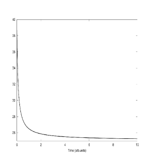
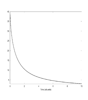
Figure 2 μ 𝜇 \mu ν 𝜈 \nu
Figure 2: The mean value of the fractional binomial process 𝔼 𝒩 ν ( t ) 𝔼 superscript 𝒩 𝜈 𝑡 \mathbb{E}\,\mathcal{N}^{\nu}(t) ( λ , μ ) = ( 0 , 1 ) 𝜆 𝜇 0 1 (\lambda,\mu)=(0,1) ( λ , μ ) = ( 1 , 0 ) 𝜆 𝜇 1 0 (\lambda,\mu)=(1,0) N = 100 𝑁 100 N=100 M = 40 𝑀 40 M=40 ν = 0.7 𝜈 0.7 \nu=0.7
The variance can be easily determined using (2.11
𝕍 ar 𝒩 d ν ( t ) = 𝕍 ar subscript superscript 𝒩 𝜈 𝑑 𝑡 absent \displaystyle\mathbb{V}\text{ar}\,\mathcal{N}^{\nu}_{d}(t)={} M ( M − 1 ) E ν , 1 ( − 2 μ t ν ) + M E ν , 1 ( − μ t ν ) 𝑀 𝑀 1 subscript 𝐸 𝜈 1
2 𝜇 superscript 𝑡 𝜈 𝑀 subscript 𝐸 𝜈 1
𝜇 superscript 𝑡 𝜈 \displaystyle M(M-1)E_{\nu,1}\left(-2\mu t^{\nu}\right)+ME_{\nu,1}\left(-\mu t^{\nu}\right) (3.2)
− M 2 [ E ν , 1 ( − μ t ν ) ] 2 , t ≥ 0 , ν ∈ ( 0 , 1 ] , formulae-sequence superscript 𝑀 2 superscript delimited-[] subscript 𝐸 𝜈 1
𝜇 superscript 𝑡 𝜈 2 𝑡
0 𝜈 0 1 \displaystyle-M^{2}\left[E_{\nu,1}\left(-\mu t^{\nu}\right)\right]^{2},\qquad t\geq 0,\>\nu\in(0,1],
and this reduces for ν = 1 𝜈 1 \nu=1 Bailey (1964 ) , page 91, formula (8.32)):
𝕍 ar 𝒩 d 1 ( t ) = M e − μ t ( 1 − e − μ t ) . 𝕍 ar subscript superscript 𝒩 1 𝑑 𝑡 𝑀 superscript 𝑒 𝜇 𝑡 1 superscript 𝑒 𝜇 𝑡 \displaystyle\mathbb{V}\text{ar}\,\mathcal{N}^{1}_{d}(t)=Me^{-\mu t}\left(1-e^{-\mu t}\right). (3.3)
Furthermore, the extinction probability of the fractional linear pure death
process 𝒩 d ν ( t ) subscript superscript 𝒩 𝜈 𝑑 𝑡 \mathcal{N}^{\nu}_{d}(t) t ≥ 0 𝑡 0 t\geq 0 Orsingher et al. (2010 ) , page 73, formula (2.1)),
Pr { 𝒩 d ν ( t ) = 0 | 𝒩 d ν ( 0 ) = M } = ∑ h = 0 M ( M h ) ( − 1 ) h E ν , 1 ( − h μ t ν ) , t ≥ 0 , formulae-sequence Pr conditional-set subscript superscript 𝒩 𝜈 𝑑 𝑡 0 subscript superscript 𝒩 𝜈 𝑑 0 𝑀 superscript subscript ℎ 0 𝑀 binomial 𝑀 ℎ superscript 1 ℎ subscript 𝐸 𝜈 1
ℎ 𝜇 superscript 𝑡 𝜈 𝑡 0 \displaystyle\text{Pr}\{\mathcal{N}^{\nu}_{d}(t)=0|\mathcal{N}^{\nu}_{d}(0)=M\}=\sum_{h=0}^{M}\binom{M}{h}(-1)^{h}E_{\nu,1}\left(-h\mu t^{\nu}\right),\qquad t\geq 0, (3.4)
can also be derived directly from (2.21
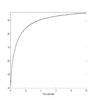
For the saturable fractional pure birth process 𝒩 b ν ( t ) subscript superscript 𝒩 𝜈 𝑏 𝑡 \mathcal{N}^{\nu}_{b}(t)
𝔼 𝒩 b ν ( t ) = N − ( N − M ) E ν , 1 ( − λ t ν ) . 𝔼 subscript superscript 𝒩 𝜈 𝑏 𝑡 𝑁 𝑁 𝑀 subscript 𝐸 𝜈 1
𝜆 superscript 𝑡 𝜈 \displaystyle\mathbb{E}\,\mathcal{N}^{\nu}_{b}(t)=N-\left(N-M\right)E_{\nu,1}\left(-\lambda t^{\nu}\right). (3.5)
Figure 2 λ 𝜆 \lambda ν 𝜈 \nu 2.11
𝕍 ar 𝒩 b ν ( t ) = 𝕍 ar subscript superscript 𝒩 𝜈 𝑏 𝑡 absent \displaystyle\mathbb{V}\text{ar}\,\mathcal{N}^{\nu}_{b}(t)={} [ M ( M − 1 ) − N ( N − 1 ) ] E ν , 1 ( − 2 λ t ν ) delimited-[] 𝑀 𝑀 1 𝑁 𝑁 1 subscript 𝐸 𝜈 1
2 𝜆 superscript 𝑡 𝜈 \displaystyle\left[M(M-1)-N(N-1)\right]E_{\nu,1}\left(-2\lambda t^{\nu}\right) (3.6)
− ( N − M ) ( 4 N − 1 ) E ν , 1 ( − λ t ν ) − ( M − N ) 2 [ E ν , 1 ( − λ t ν ) ] 2 . 𝑁 𝑀 4 𝑁 1 subscript 𝐸 𝜈 1
𝜆 superscript 𝑡 𝜈 superscript 𝑀 𝑁 2 superscript delimited-[] subscript 𝐸 𝜈 1
𝜆 superscript 𝑡 𝜈 2 \displaystyle-(N-M)(4N-1)E_{\nu,1}\left(-\lambda t^{\nu}\right)-(M-N)^{2}\left[E_{\nu,1}\left(-\lambda t^{\nu}\right)\right]^{2}.
As t → ∞ → 𝑡 t\rightarrow\infty
𝔼 𝒩 b ν ( t ) ⟶ N ⟶ 𝔼 subscript superscript 𝒩 𝜈 𝑏 𝑡 𝑁 \mathbb{E}\,\mathcal{N}^{\nu}_{b}(t)\longrightarrow N (3.7)
and
𝕍 ar 𝒩 b ν ( t ) ⟶ 0 ⟶ 𝕍 ar subscript superscript 𝒩 𝜈 𝑏 𝑡 0 \mathbb{V}\text{ar}\,\mathcal{N}^{\nu}_{b}(t)\longrightarrow 0 (3.8)
as expected.
We now determine the state probabilities p n , b ν ( t ) = Pr { 𝒩 b ν ( t ) = n | 𝒩 b ν ( 0 ) = M } superscript subscript 𝑝 𝑛 𝑏
𝜈 𝑡 Pr subscript superscript 𝒩 𝜈 𝑏 𝑡 conditional 𝑛 subscript superscript 𝒩 𝜈 𝑏 0 𝑀 p_{n,b}^{\nu}(t)=\Pr\{\mathcal{N}^{\nu}_{b}(t)=n|\mathcal{N}^{\nu}_{b}(0)=M\} μ = 0 𝜇 0 \mu=0 Orsingher and Polito (2010 ) , and is given as
p n , b ν ( t ) = { ∏ j = M n − 1 λ j ∑ m = M n 1 ∏ l = M , l ≠ m n ( λ l − λ m ) E ν , 1 ( − λ m t ν ) , M < n ≤ N , E ν , 1 ( − λ M t ν ) , n = M . superscript subscript 𝑝 𝑛 𝑏
𝜈 𝑡 cases superscript subscript product 𝑗 𝑀 𝑛 1 subscript 𝜆 𝑗 superscript subscript 𝑚 𝑀 𝑛 1 superscript subscript product formulae-sequence 𝑙 𝑀 𝑙 𝑚 𝑛 subscript 𝜆 𝑙 subscript 𝜆 𝑚 subscript 𝐸 𝜈 1
subscript 𝜆 𝑚 superscript 𝑡 𝜈 𝑀 𝑛 𝑁 subscript 𝐸 𝜈 1
subscript 𝜆 𝑀 superscript 𝑡 𝜈 𝑛 𝑀 p_{n,b}^{\nu}(t)=\begin{cases}\prod_{j=M}^{n-1}\lambda_{j}\sum_{m=M}^{n}\frac{1}{\prod_{l=M,l\neq m}^{n}(\lambda_{l}-\lambda_{m})}E_{\nu,1}\left(-\lambda_{m}t^{\nu}\right),&M<n\leq N,\\
E_{\nu,1}\left(-\lambda_{M}t^{\nu}\right),&n=M.\end{cases} (3.9)
Substituting the rates λ j = λ ( N − j ) subscript 𝜆 𝑗 𝜆 𝑁 𝑗 \lambda_{j}=\lambda(N-j)
p n , b ν superscript subscript 𝑝 𝑛 𝑏
𝜈 \displaystyle p_{n,b}^{\nu} ( t ) 𝑡 \displaystyle(t) (3.10)
= \displaystyle={} ∏ j = M n − 1 λ ( N − j ) ∑ m = M n E ν , 1 ( − λ ( N − m ) t ν ) ∏ l = M , l ≠ m n ( λ ( N − l ) − λ ( N − m ) ) superscript subscript product 𝑗 𝑀 𝑛 1 𝜆 𝑁 𝑗 superscript subscript 𝑚 𝑀 𝑛 subscript 𝐸 𝜈 1
𝜆 𝑁 𝑚 superscript 𝑡 𝜈 superscript subscript product formulae-sequence 𝑙 𝑀 𝑙 𝑚 𝑛 𝜆 𝑁 𝑙 𝜆 𝑁 𝑚 \displaystyle\prod_{j=M}^{n-1}\lambda(N-j)\sum_{m=M}^{n}\frac{E_{\nu,1}\left(-\lambda(N-m)t^{\nu}\right)}{\prod_{l=M,l\neq m}^{n}(\lambda(N-l)-\lambda(N-m))}
= \displaystyle={} ∑ m = M n ( N − M ) ( N − M − 1 ) … ( N − n + 1 ) ( m − M ) ( m − M − 1 ) … ( m − m + 1 ) ( m − m − 1 ) … ( m − n ) superscript subscript 𝑚 𝑀 𝑛 𝑁 𝑀 𝑁 𝑀 1 … 𝑁 𝑛 1 𝑚 𝑀 𝑚 𝑀 1 … 𝑚 𝑚 1 𝑚 𝑚 1 … 𝑚 𝑛 \displaystyle\sum_{m=M}^{n}\frac{(N-M)(N-M-1)\dots(N-n+1)}{(m-M)(m-M-1)\dots(m-m+1)(m-m-1)\dots(m-n)}
× E ν , 1 ( − λ ( N − m ) t ν ) absent subscript 𝐸 𝜈 1
𝜆 𝑁 𝑚 superscript 𝑡 𝜈 \displaystyle\times E_{\nu,1}\left(-\lambda(N-m)t^{\nu}\right)
= \displaystyle={} ∑ m = M n ( N − M ) ! ( N − n ) ! ( m − M ) ! ( n − m ) ! ( − 1 ) n − m E ν , 1 ( − λ ( N − m ) t ν ) superscript subscript 𝑚 𝑀 𝑛 𝑁 𝑀 𝑁 𝑛 𝑚 𝑀 𝑛 𝑚 superscript 1 𝑛 𝑚 subscript 𝐸 𝜈 1
𝜆 𝑁 𝑚 superscript 𝑡 𝜈 \displaystyle\sum_{m=M}^{n}\frac{(N-M)!}{(N-n)!(m-M)!(n-m)!}(-1)^{n-m}E_{\nu,1}\left(-\lambda(N-m)t^{\nu}\right)
= \displaystyle={} ( N − M N − n ) ∑ m = M n ( n − M m − M ) ( − 1 ) n − m E ν , 1 ( − λ ( N − m ) t ν ) , M ≤ n ≤ N . binomial 𝑁 𝑀 𝑁 𝑛 superscript subscript 𝑚 𝑀 𝑛 binomial 𝑛 𝑀 𝑚 𝑀 superscript 1 𝑛 𝑚 subscript 𝐸 𝜈 1
𝜆 𝑁 𝑚 superscript 𝑡 𝜈 𝑀
𝑛 𝑁 \displaystyle\binom{N-M}{N-n}\sum_{m=M}^{n}\binom{n-M}{m-M}(-1)^{n-m}E_{\nu,1}\left(-\lambda(N-m)t^{\nu}\right),\quad M\leq n\leq N.
This and formula (3.5 T j ν superscript subscript 𝑇 𝑗 𝜈 T_{j}^{\nu} j 𝑗 j ( j + 1 ) 𝑗 1 (j+1)
Pr { T j ν ∈ d s } = λ ( N − j ) s ν − 1 E ν , ν ( − λ ( N − j ) s ν ) d s , j ≥ M , s ≥ 0 . formulae-sequence Pr superscript subscript 𝑇 𝑗 𝜈 d 𝑠 𝜆 𝑁 𝑗 superscript 𝑠 𝜈 1 subscript 𝐸 𝜈 𝜈
𝜆 𝑁 𝑗 superscript 𝑠 𝜈 d 𝑠 formulae-sequence 𝑗 𝑀 𝑠 0 \displaystyle\Pr\{T_{j}^{\nu}\in\mathrm{d}s\}=\lambda(N-j)s^{\nu-1}E_{\nu,\nu}\left(-\lambda(N-j)s^{\nu}\right)\mathrm{d}s,\qquad j\geq M,\>s\geq 0. (3.11)
The figure below shows the sample paths of the saturable fractional (bottom) and classical (top) linear pure birth processes. Apparently, the proposed model naturally includes processes or populations that saturate faster than the classical linear pure birth process. The figure also indicates that saturation of the fractional binomial process is faster due to the explosive growth/birth bursts at small times and as ν → 0 → 𝜈 0 \nu\to 0 Cahoy and Polito (2011 ) .
Figure 3: Sample trajectories of classical (top) and fractional (bottom) saturable linear pure birth processes using values ( N , M , λ , ν ) = ( 100 , 5 , 1 , 1 ) 𝑁 𝑀 𝜆 𝜈 100 5 1 1 (N,M,\lambda,\nu)=(100,5,1,1) ( N , M , λ , ν ) = ( 100 , 5 , 1 , 0.75 ) 𝑁 𝑀 𝜆 𝜈 100 5 1 0.75 (N,M,\lambda,\nu)=(100,5,1,0.75)