Velocity-Field Theory, Boltzmann’s Transport Equation, Geometry and Emergent Time

Abstract

Boltzmann equation describes the time development of the velocity distribution in the continuum fluid matter. We formulate the equation using the field theory where the velocity-field plays the central role. The properties of the fluid matter (fluid particles) appear as the density and the viscosity. Statistical fluctuation is examined, and is clearly discriminated from the quantum effect. The time variable is emergently introduced through the computational process step. Besides the ordinary potential, the general velocity potential is introduced. The collision term, for the Higgs-type velocity potential, is explicitly obtained and the (statistical) fluctuation is closely explained. The system is generally non-equilibrium. The present field theory model does not conserve energy and is an open-system model. One dimensional Navier-Stokes equation, i.e., Burgers equation, appears. In the latter part of the text, we present a way to directly define the distribution function by use of the geometry, appearing in the energy expression, and Feynman’s path-integral.

Laboratory of Physics, School of Food and Nutritional Sciences, University of Shizuoka, Yada 52-1, Shizuoka 422-8526, Japan

Key Words :  Boltzmann equation; velocity field theory; statistical fluctuation; computational step number; open system; geometry.

1 Introduction

Boltzmann equation was introduced to explain the second law of the thermodynamics in the dynamical way, in 1872, by Boltzmann. We considers the (visco-elastic) fluid matter and examine the dynamical behavior using the velocity-field theory. The scale size we consider is far bigger than the atomic scale ($\sim 10^{-10}$m) and is smaller than or nearly equal to the optical microscope scale ($\sim 10^{-6}$m). The equation describes the temporal development of the distribution function $f(t,{\bf x},{\bf v})$ which shows the probability of a fluid-molecule (particle) having the velocity ${\bf v}$ at the space ${\bf x}$ and time $t$.

We reformulate the Boltzmann equation using the field theory of the velocity field ${\bf u}({\bf x},\leavevmode\nobreak\ ^{\prime}t^{\prime})$. Basically it is based on the minimal energy principle. We do not introduce time $t$. Instead of $t$, we use the computational step number $n$. The system we consider consists of the huge number of fluid-particles (molecules) and the physical quantities, such as energy and entropy, are the statistically-averaged ones. It is not obtained by the deterministic way like the classical (Newton) mechanics. We introduce the statistical ensemble by using the well-established field-theory method, the background-field method[6, 7]. Renormalization phenomenon occurs not from the quantum effect but from the statistical fluctuation due to the inevitable uncertainty caused by 1) the step-wise (discrete-time) formulation and 2) the continuum formulation for the space (of the real matter world).

After the development of the string and D-brane theories[8, 9], one general relation, between the 4-dimensional(4D) conformal theories and the 5D gravitational theories, was proposed. The 5D gravitational theories are asymptotically AdS₅[10, 11, 12]. The proposal claims the quantum behavior of the 4D theories is obtainable by the classical analysis of the 5D gravitational ones. The development along the extra axis can be regarded as the renormalization flow. This approach (called AdS/CFT) has been providing non-perturbative studies in several branches: quark-gluon plasma physics, heavy-ion collisions, non-equilibrium statistical mechanics, superconductivity, superfluidity[13, 14]. Especially, as the most relevant to the present work, the connection with the hydrodynamics is important[15]. When a black hole is given a perturbation, the effect decays as the relaxation phenomenon. The transport coefficients, such as viscosities, speed of sound, thermal conductivity, are important physical quantities.

The dissipative system we consider is characterized by the dissipation of energy (heat). Even for the particle classical (Newton) mechanics, the notion of energy is somewhat obscure when the dissipation occurs. We consider the movement of a particle under the influence of the friction force, $F_{\mbox{friction}}$. The emergent energy, $E(x(t),\dot{x}(t))$, during the period [t₁, t₂] can not be written as the following form.

$$\int_{x_{1}}^{x_{2}}F_{\mbox{friction}}\leavevmode\nobreak\ dx=\left[E(x(t),\dot{x}(t))\right]_{t_{1}}^{t_{2}}=E|_{t_{2}}-E|_{t_{1}}\ ,\ x_{1}=x(t_{1})\ ,\ x_{2}=x(t_{2})\ ,$$ (1)

where $x(t)$ is the orbit (path) of the particle. It depends on the path (or orbit) itself. It cannot be written as the form of difference between some quantity ($E(t)$) at time t₁ and t₂. In this situation, we realize the time itself should be re-considered when the dissipation occurs. Owing to Einstein’s idea of ”space-time democracy”, we have stuck to the standpoint that space and time should be treated on the equal footing. We present here the step-wise approach to the time-development.

We do not use time variable. Instead we use the computational-process step number $n$. Hence the increasing of the number $n$ is identified as the time development. The connection between step $n$ and step $n-1$ is determined by the minimal energy principle. In this sense, time is ”emergent” from the minimal energy principle. The direction of flow (arrow of time) is built in from the beginning. The usefulness of the step number approach (discrete Morse flow method) is shown in the text. The step-wise treatment makes the ’time’ direction manipulation more skillful and fruitful.

In the latter part of this paper, an approach to the statistically- averaging procedure , based on the geometry of the mechanical dynamics, is presented.

The content is described as follows. The step-wise dynamical equation is presented in Sec.2. We start with the n-th step energy functional. By regarding n steps as the time t_n, we derive Burgers equation (1 dim Navier-Stokes equation). In Sec.3, the orbit (path) of the fluid particle is explained in this step-wise formalism. The total energy and the energy rate are also explained. The statistical fluctuation is closely explained in Sec.4. Especially the difference from the quantum effect is stressed. Using the path-integral, we take into account the fluctuation effect. Owing to the present velocity-field formalism, we can obtain Boltzmann’s equation, as described in Sec.5, up to the collision term. This step-wise approach is applied to the mechanical system in Sec.6. We take a simple dissipative model: the harmonic oscillator with friction. The trajectory is solved in the step-wise way. We find the total energy changes as the step proceeds. From the n-step energy expression we can extract the geometrical structure (the metric) of the trajectory. The metric is used, in Sec.7, to define the statistical ensemble of the system of N viscous particles in one space dimension. We propose some models using the geometrically-basic quantities: the length and the area. Conclusion is given in Sec.8. Some appendices are provided to supplement the text. App.A treats (1+3) dimensional field theory in this step-wise formalism. App.B is the calculation of the statistical fluctuation effect and it supplements Sec.4. A few simulation results of the frictional harmonic oscillator (Sec.6) are shown in App.C. An additional mechanical model (Spring-Block model) is described with the calculation result in App.D.

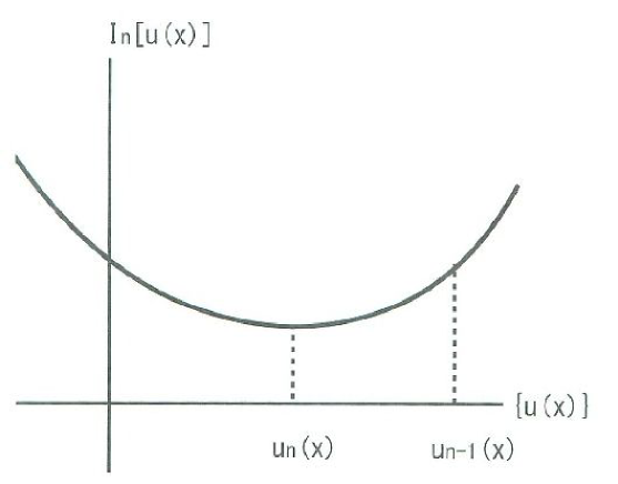
Figure 1: The energy functional $I_{n}[u(x)]$, (2), of the velocity-field $u(x)$.

2 Emergent Time and Diffusion (Heat) Equation

We consider 1 dimensional viscous fluid , and the velocity field $\{u(x);-\infty<x<\infty\}$ describes the velocity distribution in the 1 dim space. Let us take the following energy functional[2, 3] of the velocity-field u(x),

$$I_{n}[u(x);u_{n-1}(x),\sigma_{n-1}(x),{\tilde{\rho}}_{n-1}(x)]=$$

$${\int dx}\{\frac{\sigma_{n-1}}{2{\tilde{\rho}}_{n-1}}(\frac{du}{dx})^{2}+V(u)+u\frac{dV^{1}(x)}{dx}+\frac{1}{2h}(u-u_{n-1})^{2}\}+I_{n}^{0}\ ,\ V(u)=\frac{m^{2}}{2}u^{2}+\frac{\lambda}{4!}u^{4},$$

$$n=1,2,\cdots{\quad,}\quad u=u(x)\ ,\ u_{n-1}=u_{n-1}(x)\ ,\ \sigma_{n-1}=\sigma_{n-1}(x)\ ,\ {\tilde{\rho}}_{n-1}={\tilde{\rho}}_{n-1}(x)\ ,$$ (2)

where $u_{n-1}(x),{\tilde{\rho}}_{n-1}(x)$ and $\sigma_{n-1}(x)$ are the step (n-1) distributions of the velocity, the mass-density and the viscosity respectively. $u(x)$ is the general velocity-distribution and becomes $u_{n}(x)$ by the minimal energy principle. $I_{n}^{0}$ is a ’constant’ term which is independent of $u(x)$. Later we will fix it(eq.(23)). $m^{2}$ is a parameter with the dimension of the mass density: (the mass of the fluid-particle)/ 2$l$. The quantity $I_{n}$, (2), has the physical dimension of the energy. The velocity potential $V(u)$ has the mass term and the 4-body interaction term. $V^{1}(x)$ is the (ordinary) position-dependent potential. $\frac{dV^{1}(x)}{dx}$ is the external source (force) in this velocity-field theory. $h$ is a constant which can be regarded as the time-separation for one step. $u_{n-1}(x),\sigma_{n-1}(x)$ and ${\tilde{\rho}}_{n-1}(x)$ are given distributions at the (n-1)-th step evaluation. The n-th step velocity field $u_{n}(x)$ is given by the minimal principle of the n-th energy functional $I_{n}(u)$: $\delta I_{n}/\delta u(x)=0$ at $u(x)=u_{n}(x)$. This approach is callled ”discrete Morse flows method”[2, 3, 4].

We may restrict the space region as $-l\leq x\leq l$. The variation equation $\delta I_{n}(u)=0(u(x)\rightarrow u(x)+\delta u(x))$ gives

$$\frac{1}{h}(u_{n}(x)-u_{n-1}(x))=\frac{d}{dx}\left(\frac{\sigma_{n-1}}{{\tilde{\rho}}_{n-1}}\frac{du_{n}}{dx}\right)-\frac{\delta V(u_{n})}{\delta u_{n}}-\frac{dV^{1}(x)}{dx}{\quad,}$$

$$\left.\frac{\sigma_{n-1}}{{\tilde{\rho}}_{n-1}}\frac{du_{n}}{dx}\right|_{x=-l,l}\ =\ 0,\quad\quad\quad\quad\frac{\delta V(u)}{\delta u}=m^{2}u+\frac{\lambda}{3!}u^{3}{\quad,}$$ (4)

where we have replaced the minimal solution by $u_{n}$. From this definition of $u_{n}(x)$, we have the relation:

$$I_{n}[{u_{n}}]\quad\leq\quad I_{n}[u_{n-1}]{\quad.}$$ (5)

See Fig.1. From the ordinary (continuous time) experience, we expect $I_{n}[{u_{n}}]\ \leq\ I_{n-1}[u_{n-1}]$. This relation does not hold. Because $I_{n}[{u_{n}}]$ is the n-step energy of the system, this situation makes the energy calculation more tractable.

The eq. (4) describes the n-th step velocity field $u_{n}(x)$ in terms of $u_{n-1}(x)$ and vice versa. Hence it can be used for the computer simulation.

We here introduce the discrete time variable $t_{n}$ as the step number n of $u_{n}$.

$$t_{n}=nh=n{\tau_{0}}\times(\frac{h}{{\tau_{0}}}){\quad,}\quad{\tau_{0}}\equiv h\sqrt{\lambda\sigma_{0}}/|m|{\quad,}\quad n=1,\ 2,\ \cdots$$

$$t_{0}\equiv 0{\quad,}$$ (6)

where $\sigma_{0}$ ($>0$) is the representative value (constant) of the system viscosity and ${\tau_{0}}$ is the time unit. It is useful to define the following quantity $A$.

$$A\equiv\sqrt{\lambda\sigma_{0}}/|m|{\quad,}\quad\mbox{[$A$]=TM/L}$$

$${\tilde{t}}_{n}\equiv A\cdot t_{n}=n{\tau_{0}}{\quad,}\quad{\tau_{0}}=A\cdot h{\quad,}\quad\mbox{[${\tilde{t}}_{n}$]=[${\tau_{0}}$]=T}{\quad.}$$ (7)

The eq.(4) is, in terms of the ’renewed’ field $u(x,t)$, expressed as

$$\frac{1}{h}(u(x,t_{n-1}+h)-u(x,t_{n-1}))=$$

$$\frac{\partial}{\partial x}\left(\frac{\sigma(x,t_{n-1})}{{\tilde{\rho}}(x,t_{n-1})}\frac{\partial u(x,t_{n})}{\partial x}\right)-\frac{\delta V(u(x,t_{n}))}{\delta u(x,t_{n})}-\frac{\partial V^{1}(x)}{\partial x}{\quad,}$$ (8)

where we use $u(x,t_{n})\equiv u_{n}(x),\ t_{n}=t_{n-1}+h$. As $h\ \rightarrow\ 0$, we obtain

$$\frac{\partial u(x,t)}{\partial t}=\frac{\partial}{\partial x}\left(\frac{\sigma(x,t)}{{\tilde{\rho}}(x,t)}\frac{\partial u(x,t)}{\partial x}\right)-\frac{\delta V(u(x,t))}{\delta u(x,t)}-\frac{\partial V^{1}(x)}{\partial x}{\quad,}$$ (9)

where we have replaced both $t_{n}$ and $t_{n-1}$ by $t$. This is, when $\sigma/{\tilde{\rho}}$=const, 1 dim diffusion equation with the potential $V(u)$.

We remind that the variational principle for the n-step energy functional $I_{n}[u(x)]$   (2), $\delta I_{n}=I_{n}[u+\delta u]-I_{n}[u]=0$, gives $u_{n}(x)$ for the given $u_{n-1}(x),\sigma_{n-1}(x)$ and ${\tilde{\rho}}_{n-1}(x)$. We regard the increase of the step number as the time development. Taking into account the fact that, at the (n-1)th-step, the matter-particle at the point $x$ flows at the speed of $u_{n-1}(x)$, the energy functional $I_{n}$, (2), should be replaced by the following one[2, 3].

$${\tilde{I}}_{n}[u(x)]={\int dx}\{\frac{\sigma_{n-1}}{2{\tilde{\rho}}_{n-1}}(\frac{du}{dx})^{2}+V(u)+u\frac{dV^{1}(x)}{dx}$$

$$+\frac{1}{2h}(u(x+Ah\leavevmode\nobreak\ u_{n-1})-u_{n-1})^{2}\}+{\tilde{I}}_{n}^{0}{\quad,}$$

$$V(u)=\frac{m^{2}}{2}u^{2}+\frac{\lambda}{4!}u^{4},\quad n=1,2,\cdots\ ,$$

$$u=u(x)\ ,\ u_{n-1}=u_{n-1}(x)\ ,\ \sigma_{n-1}=\sigma_{n-1}(x)\ ,\ {\tilde{\rho}}_{n-1}={\tilde{\rho}}_{n-1}(x)\ .$$ (10)

Note that $u(x)-u_{n-1}(x)$ in eq.(2) is replaced by $u(x+Ah\leavevmode\nobreak\ u_{n-1}(x))-u_{n-1}(x)$. (${\tau_{0}}=Ah$ is the time difference between 1 step. ) For the simple case of no potential, $V=0$ , and no external force, $\frac{dV^{1}}{dx}=0$,

$$J_{n}[u(x)]={\int dx}\{\frac{\sigma_{n-1}}{2{\tilde{\rho}}_{n-1}}(\frac{du}{dx})^{2}+\frac{1}{2h}(u(x+Ah\leavevmode\nobreak\ u_{n-1}(x))-u_{n-1}(x))^{2}\}+^{\prime}\mbox{const}^{\prime},$$ (11)

The above functional is equivalent to $I_{n}[u(x)]$ with the potential.

$$V(u)=A(u(x)-u_{n-1}(x))u_{n-1}(x)\frac{du(x)}{dx}+O(h){\quad.}$$ (12)

where we consider the case of sufficiently-small $h$. Eq.(4) gives us the following equation as the minimal equation for $J_{n}[u]:\ \delta J_{n}[u]=0$

$$\frac{1}{h}(u_{n}(x)-u_{n-1}(x))=\frac{d}{dx}X[u_{n}(x),u_{n-1}(x)]-A\leavevmode\nobreak\ u_{n-1}(x)\frac{du_{n}(x)}{dx}{\quad,}$$

$$X[u_{n}(x),u_{n-1}(x)]|_{x=-l,l}\ =\ 0\ ,$$

$$X[u_{n}(x),u_{n-1}(x)]=A(u_{n}(x)-u_{n-1}(x))u_{n-1}(x)+\frac{\sigma_{n-1}}{{\tilde{\rho}}_{n-1}}\frac{du_{n}}{dx}\ .$$ (14)

Hence the step-wise recursion relation (4) is corrected as

$$\mbox{[Comp 1]}\quad u_{n}(x)\ \mbox{Equation}\quad\quad\quad\quad\quad\quad\quad\quad\quad\quad\quad\quad\quad\quad\quad\quad$$

$$\frac{1}{h}(u_{n}(x)-u_{n-1}(x))+A\leavevmode\nobreak\ u_{n-1}(x)\frac{d{u_{n}}(x)}{dx}$$

$$=\frac{d}{dx}\left(X[u_{n}(x),u_{n-1}(x)]\right)-\frac{\delta V(u_{n})}{\delta u_{n}}-\frac{dV^{1}(x)}{dx}\ ,$$

$$X[u_{n}(x),u_{n-1}(x)]|_{x=-l,l}\ =\ 0{\quad.}$$ (15)

This equation is obtained by $(\delta{\tilde{I}}_{n}[u]/\delta u)|_{u_{n}}=0$.

As done before, let us replace the step number $n$ by the discrete time $t_{n}=nh$. Taking the continuous time limit (${\tau_{0}}=Ah\ \rightarrow\ 0$), we obtain

$$A\frac{\partial u(x,t)}{\partial{\tilde{t}}}+Au(x,t)\frac{\partial u(x,t)}{\partial x}=\frac{\partial}{\partial x}\left(\frac{\sigma(x,t)}{{\tilde{\rho}}(x,t)}\frac{\partial u(x,t)}{\partial x}\right)-\frac{\delta V(u(x,t))}{\delta u(x,t)}-\frac{\partial V^{1}(x)}{\partial x}\ ,$$

$$\left.\frac{\sigma(x,t)}{{\tilde{\rho}}(x,t)}\frac{\partial u(x,t)}{\partial x}\right|_{x=-l,l}=\ 0{\quad,}$$ (16)

where two continuous times ($t$ and ${\tilde{t}}=At$) are used: $t_{n}=nh\rightarrow t$ and ${\tilde{t}}_{n}=nAh=n{\tau_{0}}\rightarrow{\tilde{t}}(=A\leavevmode\nobreak\ t)$ as $n\rightarrow\infty$. This is , when $\sigma/{\tilde{\rho}}$=const, Burgers equation (with the velocity potential $V(u)$ and the external force $\frac{\partial V^{1}}{\partial x}$) and is considered to be 1 dimensional Navier-Stokes equation. Note that the non-linear term in the LHS of eq.(16) appears not from the potential ( velocity-field interaction) but from the change $u(x)$ in (2) to $u(x+Ahu_{n-1})$ in (10), namely, the consistency between the (space) coordinate $x$ and the velocity field $u(x)$ in the step-flow. The differential operator: $\frac{\partial}{\partial{\tilde{t}}}+u\frac{\partial}{\partial x}\equiv\frac{D}{D{\tilde{t}}}$, appearing in LHS, is called Lagrange derivative. The relations between $\sigma_{n-1}$ and $\sigma_{n}$, and ${\tilde{\rho}}_{n-1}$ and ${\tilde{\rho}}_{n}$, which describe their step-flow (’time’-development), are given in Sec.5.

The equation (16), for the massless case $m=0$, is invariant under the global scale transformation.

$$t\quad\rightarrow\quad{\rm e}^{2\varepsilon}t{\quad,}\quad x\quad\rightarrow\quad{\rm e}^{\varepsilon}x{\quad,}$$

$$\frac{\partial}{\partial x}=\partial_{x}\quad\rightarrow\quad{\rm e}^{-\varepsilon}\partial_{x}{\quad,}\quad\frac{\partial}{\partial t}=\partial_{t}\quad\rightarrow\quad{\rm e}^{-2\varepsilon}\partial_{t}{\quad,}$$

$$u(x,t)\quad\rightarrow\quad{\rm e}^{-\varepsilon}u({\rm e}^{\varepsilon}x,{\rm e}^{2\varepsilon}t){\quad,}\quad\frac{\sigma(x,t)}{{\tilde{\rho}}(x,t)}\quad\rightarrow\quad\frac{\sigma({\rm e}^{\varepsilon}x,{\rm e}^{2\varepsilon}t)}{{\tilde{\rho}}({\rm e}^{\varepsilon}x,{\rm e}^{2\varepsilon}t)}{\quad,}$$

$$V^{1}(x)\ \rightarrow\ {\rm e}^{-2\varepsilon}V^{1}({\rm e}^{\varepsilon}x)\ ,\ V(u(x,t))\ \rightarrow\ {\rm e}^{-2\varepsilon}V(u({\rm e}^{\varepsilon}x,{\rm e}^{2\varepsilon}t))\ (\lambda\ \rightarrow\ {\rm e}^{-2\varepsilon}\lambda){\quad,}$$ (17)

where $\varepsilon$ is the real constant parameter. When it is small : $|\varepsilon|\ll 1$, the variation $\delta u$ is given by

$$\delta u=\varepsilon\{-u+x\leavevmode\nobreak\ \partial_{x}u+2t\leavevmode\nobreak\ \partial_{t}u\}+O(\varepsilon^{2}){\quad,}$$ (18)

For simplicity, we explain in one space-dimension (dim). The generalization to 2 dim and 3 dim is straightforward. Furthermore the ordinary field theory (not using the velocity field but the particle field) is described by this step-wise approach in App.A.

3 Space Orbit (Path) and Total Energy

The space coordinate $x$ always appears in the velocity field $u_{n}(x)$. We can introduce the n-th step space coordinate $x_{n}$ as

$$u_{n}(x_{n})=\frac{x_{n+1}-x_{n}}{{\tau_{0}}}{\quad,}\quad n=0,1,2,\cdots$$

$$x_{n+1}=x_{n}+{\tau_{0}}u_{n}(x_{n}){\quad,}$$ (19)

where $x_{0}$ is a given initial position and ${\tau_{0}}=h\sqrt{\lambda\sigma_{0}}/|m|=hA$ in eq.(6). We can trace the position of the matter-point, which is at $x_{0}$ as the initial (0-th) step, along the step process: $x_{0},x_{1},x_{2},\cdots$. After N steps, the matter-point reaches the following point.

$$x_{N}=x_{N-1}+{\tau_{0}}u_{N-1}(x_{N-1})=x_{0}+{\tau_{0}}\sum_{n=0}^{N-1}u_{n}(x_{n}){\quad.}$$ (20)

In terms of the continuous time ${\tilde{t}}=At$,

$$x(T)=x_{0}+\int_{0}^{T}u(x(t),t)d{\tilde{t}}{\quad,}$$ (21)

where $T=N\leavevmode\nobreak\ Ah,{\tilde{t}}_{n}=n\leavevmode\nobreak\ Ah=At_{n},x(t_{n})=x_{n},u(x,t_{n})=u_{n}(x)$. $x(t)$ is the orbit or path of the matter-point, at $x_{0}$ initially, ”moving” in the N steps.

At the n-th step, the total energy of the system, $E_{n}$, is given by

$$E_{n}\equiv{\tilde{I}}_{n}[u_{n}]{\quad,}\quad\mbox{where}\quad\quad\quad\quad\quad\left.\frac{\delta{\tilde{I}}_{n}[u]}{\delta u(x)}\right|_{u=u_{n}}=0{\quad,}$$

$${\tilde{I}}_{n}[u]={\int dx}\{\frac{\kappa_{n-1}}{2}(\frac{du}{dx})^{2}+V(u)+u\frac{dV^{1}}{dx}+\frac{1}{2h}(u(x+hAu_{n-1})-u_{n-1})^{2}\}+{\tilde{I}}_{n}^{0}\ ,$$

$$\kappa_{n}(x)\equiv\frac{\sigma_{n}(x)}{{\tilde{\rho}}_{n}(x)}{\quad,}\quad\quad u=u(x){\quad,}\quad u_{n-1}=u_{n-1}(x){\quad,}$$ (22)

where $\kappa_{n}=\kappa_{n}(x)$ is introduced. ${\tilde{I}}_{n}^{0}$ is taken as

$${\tilde{I}}_{n}^{0}=-{\int dx}\{u_{n}\frac{dV^{1}}{dx}+\frac{1}{2h}(u_{n}(x+hAu_{n-1})-u_{n-1})^{2}\}$$

$$+{\int dx}\{\frac{\kappa_{0}}{2}(\frac{du_{0}}{dx})^{2}+V(u_{0})+u_{0}\frac{dV^{1}}{dx}+\frac{{\tilde{\rho}}_{0}}{2}{u_{0}}^{2}\}{\quad.}$$ (23)

The above one (${\tilde{I}}_{n}^{0}$) is chosen in such a way that the total energy $E_{n}={\tilde{I}}_{n}[u_{n}]$ keeps the initial energy (the second integral of (23)) when the dissipative terms, $\frac{\kappa_{n-1}}{2}(\frac{du}{dx})^{2}$ and $V(u)$, do not appear. ${\tilde{I}}_{n}[u_{n}]$ is the n-th step dissipative energy plus the initial energy.

The system total energy $E_{n}$ generally changes as the step number, n, increases.

$$W(t_{n})\equiv\frac{dE(t_{n})}{d{\tilde{t}}_{n}}=\frac{h}{{\tau_{0}}}\frac{dE(t_{n})}{dt_{n}}\equiv\frac{{\tilde{I}}_{n+1}[u_{n+1}]-{\tilde{I}}_{n}[u_{n}]}{{\tau_{0}}}=$$

$$\frac{1}{{\tau_{0}}}{\int dx}\left\{{1\over 2}\left(\kappa_{n}(\frac{du_{n+1}}{dx})^{2}-\kappa_{n-1}(\frac{du_{n}}{dx})^{2}\right)+V(u_{n+1})-V(u_{n})+(u_{n+1}-u_{n})\frac{dV^{1}}{dx}\right.$$

$$\left.+\frac{1}{2h}\{(u_{n+1}+hAu_{n}\frac{du_{n+1}}{dx}-u_{n})^{2}-(u_{n}+hAu_{n-1}\frac{du_{n}}{dx}-u_{n-1})^{2}\}\right\}+\frac{{\tilde{I}}_{n+1}^{0}-{\tilde{I}}_{n}^{0}}{{\tau_{0}}},$$ (24)

where $E(t_{n})\equiv E_{n}$ and $W(t_{n})$ is the energy rate. From the above formula we get the expression for the energy at $t=Nh=t_{N}$.

$$E(t_{N})={\tilde{I}}_{N}[u_{N}]={\tilde{I}}_{N-1}[u_{N-1}]+{\tau_{0}}W(t_{N-1})={\tilde{I}}_{1}[u_{1}]+{\tau_{0}}\sum_{n=1}^{N-1}W(t_{n}){\quad.}$$ (25)

When we regard the process of the increasing step-number as the time development, the system generally does not conserve energy. $E(t_{n})$($={\tilde{I}}_{n}[u_{n}]$) generally changes step by step. We can physically understand that the increase or decrease of the total system energy is given or subtracted by the outside (environment). The energy functional (10) describes the open-system dynamics. When $E(t_{n})$ satisfies

$$W(t_{n})=\frac{h}{{\tau_{0}}}\frac{dE(t_{n})}{dt_{n}}\quad\rightarrow\quad W_{0}(\mbox{constant})\quad\mbox{as}\ n\rightarrow\infty{\quad,}$$ (26)

we say the system finally reaches the steady energy-state. For the special case of $W_{0}=0$, we say the system finally reaches the constant energy-state .

In Sec.6, we treat the $W_{0}=0$ case. As the example of the more general case ($W_{0}\neq 0$), another model is given in App.C.

4 Statistical Fluctuation Effect

We are considering the system of large number of matter-particles, hence the physical quantities, such as energy and entropy, are given by the statistical average. In the present approach, the system behavior $u_{n}(x)=u(x,t_{n})$ is completely determined by eq.(15) when the initial configuration $u_{0}(x)=u(x,0)$ is given. We have obtained the solution by the continuous variation $\delta u(x)$ to ${\tilde{I}}_{n}[u]$, (10). In this sense, $u_{n}(x)$ is the ’classical path’. Here we should note that the present formalism is an effective approach to calculate the physical properties of this statistical system. Approximation is made in the following points:

1)

So far as $h\neq 0$, the finite time-increment gives uncertainty to the minimal solution $u_{n}(x)$. This is because we cannot specify the minimum configuration definitely, but can only do it with finite uncertainty.

2)

We do not measure the initial $u_{0}(x)$. Hence the velocity distribution $u_{n}(x)$ fluctuates due to the initial condition ambiguity.

3)

The real fluid matter is made of many micro particles with small but non-zero size. The existence of the characteristic particle size gives uncertainty to the minimal solution in this (space-)continuum formalism. Furthermore the particle size is not constant but does distribute in the statistical way. The shape of each particle differs. The present continuum formalism has limitation to describe the real situation accurately.

4)

The system energy generally changes step by step. The present model (10) describes an open-system. It means the present system energetically interacts with the outside. Such interaction is caused by the dissipative term in (10).

We claim the fluctuation, in the present approach, comes not from the quantum effect but from the statistics due to the uncertainty which comes from the finite time-separation and the spacial distribution of size and shape of the content particles.

To take into account this fluctuation effect, we newly define the n-th energy functional $\Gamma_{n}[u(x)]=\Gamma_{n}[u(x);u_{n-1}(x),\sigma_{n-1}(x),{\tilde{\rho}}_{n-1}(x)]$ in terms of the original one ${\tilde{I}}_{n}[u(x)]$, (10), using the path-integral(in the velocity-field).

$${\rm e}^{-{\frac{1}{\alpha}}\Gamma_{n}[u_{n}(x)]}=\int\left.{\cal D}q(x){\rm e}^{-{\frac{1}{\alpha}}{\tilde{I}}_{n}[u(x)]}\right|_{u=u_{n}+\sqrt{\alpha}q}{\quad,}\quad\quad\quad\quad\quad\quad\quad\quad$$

$${\tilde{I}}_{n}[u(x)]={\int dx}\{\frac{\kappa_{n-1}}{2}(\frac{du}{dx})^{2}+V(u)+u(x)\frac{dV^{1}(x)}{dx}$$

$$+\frac{1}{2h}(u(x+hAu_{n-1})-u_{n-1})^{2}\}+{\tilde{I}}^{0}_{n},$$

$$V(u)=\frac{m^{2}}{2}u^{2}+\frac{\lambda}{4!}u^{4}{\quad,}\quad\left.\frac{\delta{\tilde{I}}_{n}[u]}{\delta u(x)}\right|_{u=u_{n}}=0{\quad.}\quad\quad\quad\quad\quad$$ (27)

In the above path-integral expression, all paths(distributions) $\{u(x);-l\leq x\leq l\}$ are taken into account.

We are considering the minimal path $u_{n}(x)$ as the dominant configuration and the small deviation $q(x)$ around it.

$$u(x)=u_{n}(x)+{\sqrt{\alpha}}q(x){\quad,}\quad|{\sqrt{\alpha}}q|\ll|u_{n}|{\quad,}\quad\left.\frac{\delta{\tilde{I}}_{n}[u]}{\delta u}\right|_{u=u_{n}}=0{\quad,}$$ (28)

In eq.(27) and eq.(28), a new expansion parameter $\alpha$ is introduced.
([$\alpha$]=[$I_{n}$]=ML²T^-2, $[q]=1/\sqrt{M}$) As the above formula shows, $\alpha$ should be small. The concrete form should be chosen depending on problem by problem. It should not include Planck constant, $\hbar$, because the fluctuation does not come from the quantum effect. Hence the parameter $\alpha$ should be chosen as

1)

the dimension is consistent,

2)

it should have the small scale parameter which characterizes the relevant physical phenomena such as the mean-free path of the fluid particle,

3)

the precise value should be best-fitted with the experimental data.

The background-field method[6, 7] tells us to do the Taylor-expansion around ${u_{n}}$.

$${\tilde{I}}_{n}[u(x)]={\tilde{I}}_{n}[u_{n}(x)+{\sqrt{\alpha}}q(x)]=\sum_{l=0}^{\infty}\alpha^{l/2}\frac{q(x)^{l}}{l!}\left.\frac{\delta^{l}{\tilde{I}}_{n}[u]}{\delta u(x)^{l}}\right|_{u_{n}}=\sum_{l=0}^{\infty}S_{l}[u_{n}]{\quad,}$$ (29)

Then the n-th energy functional, $\Gamma_{n}[u(x)]$, is expressed in the perturbed form up to the second order (w.r.t. ${\sqrt{\alpha}}$).

$${\rm e}^{-{\frac{1}{\alpha}}\Gamma_{n}[u_{n}(x)]}=\int{\cal D}q(x)\exp(-{\frac{1}{\alpha}}(S_{0}+S_{2}+O(q^{3})))={\rm e}^{-{\frac{1}{\alpha}}{\tilde{I}}_{n}[u_{n}(x)]}\times$$

$$\int{\cal D}q\exp\left[\int dx\left\{-\frac{q(x)^{2}}{2!}(\frac{\delta}{\delta u(x)})^{2}{\tilde{I}}_{n}[u]|_{u_{n}}+O(q^{3})\right\}\right]{\quad,}\quad\frac{\delta}{\delta u(x)}{\tilde{I}}_{n}[u]|_{u_{n}}=0{\quad,}$$

$$S_{0}={\tilde{I}}_{n}[u_{n}]{\quad,}\quad S_{1}=\int dxq(x)\left.\frac{\delta{\tilde{I}}_{n}[u]}{\delta u}\right|_{u_{n}}=0{\quad,}$$

$${\frac{1}{\alpha}}S_{2}=\frac{q(x)^{2}}{2!}(\frac{\delta}{\delta u(x)})^{2}{\tilde{I}}_{n}[u]|_{u_{n}}=\int dx\left[\frac{\kappa_{n-1}}{2}(\frac{dq}{dx})^{2}+\right.$$

$$\left.(\frac{m^{2}}{2}+\frac{\lambda}{2}{u_{n}}^{2})q^{2}+\frac{1}{2h}(q+hAu_{n-1}\frac{dq}{dx})^{2}\right]$$

$$\equiv\int dx\left[{1\over 2}\frac{d}{dx}(\kappa_{n-1}q\frac{dq}{dx})+{1\over 2}qDq+O(h)\right]{\quad,}$$

$$D\equiv-\frac{d}{dx}\kappa_{n-1}\frac{d}{dx}+\lambda{u_{n}}^{2}+m^{2}+\frac{1}{h}+2u_{n-1}A\frac{d}{dx}{\quad,}$$ (30)

where we make the Gaussian(quadratic, 1-loop) approximation.

$${\rm e}^{-{\frac{1}{\alpha}}\Gamma_{n}[u_{n}(x)]}={\rm e}^{-{\frac{1}{\alpha}}{\tilde{I}}_{n}[u_{n}(x)]}\times(\det D)^{-1/2}{\quad,}$$

$$(\det D)^{-1/2}=\exp\left\{-{1\over 2}{\rm Tr}\ln D\right\}=\exp\left\{{1\over 2}{\rm Tr}\int_{0}^{\infty}\frac{{\rm e}^{-\tau D}}{\tau}d\tau+\mbox{const}\right\}{\quad,}$$ (31)

where $\tau$ is called Schwinger’s proper time[16]. ([$\tau$]=[$D^{-1}$]=L/M.)

To rigorously define the inside of the above exponent, we introduce Dirac’s abstract state vector $|x>$ and $<x|$.

$$<x|{\rm e}^{-\tau D}|y>\equiv G(x,y;\tau){\quad,}$$

$$(\frac{\partial}{\partial\tau}+D)G(x,y;\tau)=0{\quad,}\quad\lim_{\tau\rightarrow+0}G(x,y;\tau)=\delta(x-y){\quad,}$$

$$D=-\frac{d}{dx}\kappa_{n-1}(x)\frac{d}{dx}+2u_{n-1}A\frac{d}{dx}-{\bar{V}}(x){\quad,}\quad{\bar{V}}(x)=-\lambda{u_{n}(x)}^{2}-m^{2}-\frac{1}{h}{\quad.}$$ (32)

$G(x,y;\tau)$ is called heat-kernel[16].

In App.B, we evaluate, for the case $\kappa_{n-1}=\epsilon^{-1}$(const) and $A=0$, $\ln(\det D)^{-1/2}={1\over 2}\int_{0}^{\infty}d\tau{\rm Tr}G(x,y)/\tau={1\over 2}\int_{0}^{\infty}d\tau\int_{-l}^{l}dx\leavevmode\nobreak\ G(x,x)/\tau$. Up to the first order of ${\bar{V}}$, the result is given by

$$\frac{l}{\sqrt{\pi}}\sqrt{\epsilon\Lambda}-\frac{1}{2\sqrt{\pi\epsilon\mu}}\int_{-l}^{l}dz\epsilon(\lambda{u_{n}}(z)^{2}+m^{2}+\frac{1}{h}){\quad,}$$ (33)

where the infrared cut-off parameter $\mu\equiv\sqrt{\sigma_{0}}/l$ and the ultraviolet cut-off parameter $\Lambda\equiv h^{-1}$ are introduced. $\epsilon^{-1}\equiv\sigma_{0}/{\tilde{\rho}}_{0}=1$. We see the mass parameter $m^{2}$ shifts under the influence of the fluctuation.

$$m^{2}\quad\rightarrow\quad m^{2}+\frac{\alpha}{\sqrt{\pi\epsilon\mu}}\epsilon\lambda=m^{2}+\alpha\lambda\sqrt{\frac{l{\tilde{\rho}}_{0}}{\pi\sigma_{0}\sqrt{\sigma_{0}}}}{\quad.}$$ (34)

And the bottom of the potential shifts as

$$V(u_{min})\quad\rightarrow\quad V(u_{min})+\alpha\left\{{1\over 2}\sqrt{\frac{\epsilon\Lambda}{\pi}}-\frac{\epsilon}{2\sqrt{\pi\epsilon\mu}}(m^{2}+\frac{1}{h})\right\}$$

$$=V(u_{min})+\alpha\sqrt{\frac{{\tilde{\rho}}_{0}}{4\pi\sigma_{0}}}\left\{\frac{1}{\sqrt{h}}-\sqrt{\frac{l}{\sqrt{\sigma_{0}}}}(m^{2}+\frac{1}{h})\right\}{\quad.}$$ (35)

The coupling $\lambda$ is also shifted by the O(${\bar{V}}^{2}$) correction. The shift of these parameters corresponds to the renormalization in the field theory[18]. In this effective approach, we have physical cut-offs $\mu$ and $\Lambda$ which are expressed by the (finite) parameters appearing in the starting energy-functional. When the functional (10) (effectively) works well, all effects of the statistical fluctuation reduces to the simple shift of the original parameters. This corresponds to the renormalizable case in the field theory. We consider this case in the following.

5 Boltzmann’s Transport Equation

5.1 Distribution function and Boltzmann’s transport equation

We use, for simplicity, the original names for the shifted parameters. The step-wise development equation (15), with $\delta V/\delta u=m^{2}u+\frac{\lambda}{3!}{u}^{3}+u_{n-1}\frac{d{u_{n}}}{dx}$ and $V^{1}=0$, is written as

$$\mbox{[Comp 1']}\quad u_{n}(x)\ \mbox{Equation}\quad\quad\quad\quad\quad\quad\quad\quad$$

$$\frac{1}{h}(u_{n}(x)-u_{n-1}(x))=\frac{d}{dx}\left(\kappa_{n-1}\frac{du_{n}}{dx}+A(u_{n}(x)-u_{n-1}(x))u_{n-1}(x)\right)$$

$$-m^{2}u_{n}-\frac{\lambda}{3!}{u_{n}}^{3}-A\leavevmode\nobreak\ u_{n-1}\frac{du_{n}}{dx}{\quad,}\quad X[u_{n}(x),u_{n-1}(x)]|_{x=-l,l}\ =\ 0{\quad,}$$

$$X[u_{n}(x),u_{n-1}(x)]=A(u_{n}(x)-u_{n-1}(x))u_{n-1}(x)+\frac{\sigma_{n-1}}{{\tilde{\rho}}_{n-1}}\frac{du_{n}}{dx}{\quad,}$$ (36)

where $\kappa_{n}(x)=\sigma_{n}(x)/{\tilde{\rho}}_{n}(x)$(eq.(22)). When the system reaches the equilibrium state after sufficient recursive computation ($n\gg 1$), we may assume $u_{n-1}(x)=u_{n}(x)\equiv{u^{\infty}}(x),\kappa_{n-1}(x)=\sigma_{n-1}(x)/{\tilde{\rho}}_{n-1}(x)=\kappa^{\infty}$(const.). ${u^{\infty}}(x)$ satisfies

$$\kappa^{\infty}\frac{d^{2}{u^{\infty}}}{dx^{2}}-m^{2}{u^{\infty}}-\frac{\lambda}{3!}({{u^{\infty}}})^{3}-A\leavevmode\nobreak\ {u^{\infty}}\frac{d{u^{\infty}}}{dx}=0{\quad,}\quad\kappa^{\infty}\equiv\frac{\sigma^{\infty}}{{\tilde{\rho}}^{\infty}}{\quad.}$$ (37)

Here we introduce the particle number density, $\rho_{n}(x)$. The continuity equation is given by

$$\mbox{[Comp 2]}\quad\rho_{n}(x)\ \mbox{Equation}\quad\quad\quad\quad\quad\quad\quad\quad$$

$$\frac{1}{h}(\rho_{n}(x)-\rho_{n-1}(x))+\frac{d}{dx}(\rho_{n-1}(x)u_{n-1}(x))=0{\quad.}$$ (38)

This relation defines the step-flow of ${\rho_{n}}(x)$.

The distribution function $f_{n}(x,v)$ is introduced in the following way. The probability for the matter particle in the space interval $x\sim x+dx$ and the velocity interval $v\sim v+dv$, at the step $n$, is given by

$$\frac{1}{{\bar{N}}_{n}}f_{n}(x,v)dxdv{\quad,}\quad{\bar{N}}_{n}\equiv\int dxdvf_{n}(x,v){\quad,}$$ (39)

where ${\bar{N}}_{n}$ is the total particle number of the system at the step $n$.[17] Then the n-th distribution ${f_{n}}(x,v)$ and the equilibrium distribution $f^{\infty}(x,v)$ are expressed as

$${u_{n}}(x)=\frac{1}{\rho_{n}(x)}\int v{f_{n}}(x,v)dv{\quad,}\quad\rho_{n}(x)=\int dvf_{n}(x,v),$$

$${u^{\infty}}(x)=\frac{1}{\rho_{\infty}(x)}\int v{f^{\infty}}(x,v)dv{\quad,}\quad\quad\quad\quad\quad\quad\quad\quad$$

$${u_{n}}(x)\rightarrow{u^{\infty}}(x)\quad\mbox{and}\quad{f_{n}}(x,v)\rightarrow{f^{\infty}}(x,v)\quad\mbox{as}\quad n\rightarrow\infty{\quad,}$$ (40)

where ${u^{\infty}}(x)$ is the equilibrium velocity distribution. The expression $u_{n}(x)$ in eq.(40) guarantees the momentum conservation at each point, $x$.

$$0={\tilde{\rho}}_{n}(x)\int dv(v-{u_{n}}(x)){f_{n}}(x,v){\quad.}$$ (41)

The recursion relation (36) is expressed, in terms of the distribution functions, as

$$\frac{1}{h}\left[{\tilde{f}}_{n}(x+hA\leavevmode\nobreak\ u_{n-1}(x),v)-{\tilde{f}}_{n-1}(x,v)\right]=$$

$$\frac{\partial}{\partial x}\left(\kappa_{n-1}(x)\frac{\partial{\tilde{f}}_{n}(x,v)}{\partial x}\right)-m^{2}{\tilde{f}}_{n}(x,v)-\frac{\lambda}{3!}{\tilde{f}}_{n}(x,v){{u_{n}}(x)}^{2}{\quad,}$$

$${\tilde{f}}_{n}(x,v)\equiv\frac{{f_{n}}(x,v)}{\rho_{n}(x)},\ {u_{n}}(x)=\frac{1}{\rho_{n}(x)}\int v{f_{n}}(x,v)dv,\ \kappa_{n-1}(x)=\frac{\sigma_{n-1}(x)}{{\tilde{\rho}}_{n-1}(x)}\ .$$ (42)

This is the Boltzmann’s transport equation for the 2-body and 4-body velocity-interactions (Higgs-type velocity potential)[17]. We can express the step-wise expression (42) in the continuous time $t$ form as in Sec.2. This is the integro-differential equation for $f_{n}(x,v)$. The right hand side (RHS) of the top equation of (42) is called the collision term.

We now introduce some physical quantities used in the non-equilibrium statistical mechanics. The entropy $S_{n}$ and the total particle-number ${\bar{N}}_{n}$ are defined by

$$S_{n}\equiv-{k_{B}}\int dv\int dxf_{n}(x,v)\ln f_{n}(x,v){\quad,}$$

$${\bar{N}}_{n}=\int dx\rho_{n}(x)=\int dx\int dvf_{n}(x,v){\quad,}$$ (43)

where ${k_{B}}$ is Boltzmann’s constant. Another physical quantities will be presented.

Besides the particle-number density $\rho_{n}(x)$, we already have introduced the mass density ${\tilde{\rho}}_{n}(x)$ at step $n$. We here consider the case of one kind particle.

$$\frac{{\tilde{\rho}}_{n}(x)}{{\rho_{n}}(x)}=m_{1}\ (\ \mbox{constant}\ ){\quad,}$$ (44)

where $m_{1}$ is the particle mass. In this case the total mass at the step $n$, $M_{n}$, is given by

$$M_{n}\equiv\int dx\leavevmode\nobreak\ {\tilde{\rho}}_{n}(x)=m_{1}\int dx\leavevmode\nobreak\ \rho_{n}(x)=m_{1}{\bar{N}}_{n}{\quad.}$$ (45)

The temperature distribution ${\cal T}_{n}(x)$, the heat current distribution $q_{n}(x)$ and the pressure $P_{n}(x)$ are given by

$$\frac{1}{2}{k_{B}}{\cal T}_{n}(x)\equiv\frac{1}{\rho_{n}(x)}\int dv\frac{m_{1}}{2}(v-{u_{n}}(x))^{2}{f_{n}}(x,v){\quad,}$$

$$q_{n}(x)\equiv\int dv\frac{m_{1}}{2}(v-{u_{n}}(x))^{3}{f_{n}}(x,v){\quad,}$$

$$P_{n}(x)\equiv m_{1}\int dv(v-{u_{n}}(x))^{2}{f_{n}}(x,v)={k_{B}}\rho_{n}(x){\cal T}_{n}(x){\quad,}$$ (46)

where ${k_{B}}$ is Boltzmann’s constant.

In this subsection, ${\cal T}_{n}(x),q_{n}(x),P_{n}(x)$ and $S_{n}$ are introduced using the distribution function $f_{n}(x,v)$. Another definition is given in the next subsection.

5.2 Viscosity, heat conductivity and renormalization

Using the transport equation (42) which $f_{n}(x,v)$ satisfies, we expect the following two equations are satisfied. The first one is the rephrasing of the Navier-Stokes equation (36).

$$\mbox{[Comp 3]}\quad P_{n}(x)\mbox{ or }{\cal T}_{n}(x)\ \mbox{Equation}\quad\quad\quad\quad\quad\quad\quad\quad$$

$$\frac{1}{h}(u_{n}(x)-u_{n-1}(x))+A\leavevmode\nobreak\ u_{n-1}\frac{du_{n}}{dx}=-\frac{1}{{\tilde{\rho}}_{n}(x)}\frac{dP_{n}(x)}{dx}{\quad.}$$ (47)

The second one is the energy equation.

$$\mbox{[Comp 4]}\quad q_{n}(x)\ \mbox{Equation}\quad\quad\quad\quad\quad\quad\quad\quad$$

$${1\over 2}{\rho_{n}}(x){k_{B}}A\{\frac{1}{h\cdot A}({\cal T}_{n}(x)-{\cal T}_{n-1}(x))+u_{n-1}\frac{d{\cal T}_{n}}{dx}\}=-\frac{dq_{n}(x)}{dx}-P_{n}(x)\frac{d{u_{n}}(x)}{dx}{\quad,}$$ (48)

where ${\cal T}_{n}=P_{n}/{k_{B}}\rho_{n}$ is defined in (47). We explain how the above two relations, (47) and (48), are valid.

We define n-th viscosity $\sigma_{n}(x)$ by the following equation.

$$\mbox{[Comp 5]}\quad\sigma_{n}(x)\ \mbox{Equation}\quad\quad\quad\quad\quad\quad\quad\quad$$

$$P_{n}(x)=-\sigma_{n}(x)\frac{du_{n}}{dx}{\quad.}$$ (49)

This gives the step-flow of $\sigma_{n}(x)$ because other two components ($P_{n}$ and $du_{n}/dx$) are already determined by $\sigma_{n-1}(x)$. Then the RHS of eq.(47) is written as

$$-\frac{1}{{\tilde{\rho}}_{n}(x)}\frac{dP_{n}(x)}{dx}=\kappa_{n}(x)\frac{d^{2}u_{n}}{dx^{2}}+\frac{1}{{\tilde{\rho}}(x)}\frac{d\sigma_{n}(x)}{dx}\frac{du_{n}}{dx}{\quad.}$$ (50)

The LHS of eq.(47) is written, using Navier-Stokes equation (36), as

$$\frac{1}{h}(u_{n}(x)-u_{n-1}(x))+A\leavevmode\nobreak\ u_{n-1}\frac{du_{n}}{dx}=$$

$$\frac{d}{dx}\left\{\kappa_{n-1}\frac{du_{n}}{dx}+A(u_{n}-u_{n-1})u_{n-1}\right\}-m^{2}u_{n}-\frac{\lambda}{3!}{u_{n}}^{3}{\quad,}\quad A=\frac{\sqrt{\lambda\sigma_{0}}}{|m|}{\quad.}$$ (51)

Generally we have some cases about the two quantities (50) and (51).

Case W1: The two quantities coincide.
In this case, the present theory is well-defined. There is no problem.

Case W2: The 2 quantities differ, but they can be equal by changing the two constants, $m^{2}$ and $\lambda$. Namely,

$$\kappa_{n}(x)\frac{d^{2}u_{n}}{dx^{2}}+\frac{1}{{\tilde{\rho}}_{n}(x)}\frac{d\sigma_{n}(x)}{dx}\frac{du_{n}}{dx}=$$

$$\frac{d}{dx}\left\{\kappa_{n-1}\frac{du_{n}}{dx}+A^{\prime}(u_{n}-u_{n-1})u_{n-1}\right\}-{m^{\prime}}^{2}u_{n}-\frac{\lambda^{\prime}}{3!}{u_{n}}^{3}{\quad,}\quad A^{\prime}=\frac{\sqrt{\lambda^{\prime}\sigma_{0}}}{|m^{\prime}|}{\quad.}$$ (52)

By identifying $m^{2}$ and $\lambda$ by $(m^{2})_{n-1}$ and $\lambda_{n-1}$, and ${m^{2}}^{\prime}$ and $\lambda^{\prime}$ by $(m^{2})_{n}$ and $\lambda_{n}$, the above equation defines the step-flow of the two constants $(m^{2})_{n}$ and $\lambda_{n}$. We can regard this flow as the renormalization flow by identifying the step-flow with thermalization to the equilibrium state.

Case W1 is the special case of W2, namely, n(’time’)-independent one. We call the both cases well-defined theory. We call other cases, where eq.(47) is not valid, ill-defined theory. The validity check of eq.(47) selects the present model, (10), well-defined or not.

Next we explain how eq.(48) is valid in the well-defined case. Noting the heat current $q_{n}(x)$ is, in the expression (46), the higher-moment of the distribution $f_{n}(x,v)$ than the pressure $P_{n}(x)$, we newly define the heat conductivity $\omega_{n}(x)$ in the same way as (49).

$$\mbox{[Comp 6]}\quad\omega_{n}(x)\ \mbox{Equation}\quad\quad\quad\quad\quad\quad\quad\quad$$

$$q_{n}(x)=\omega_{n}(x)\frac{d{\cal T}_{n}}{dx}{\quad.}$$ (53)

Noting the equation of state $P_{n}(x)={k_{B}}\rho_{n}(x){\cal T}_{n}(x)$ (46), eq.(48) is written as

$${1\over 2}\{\frac{1}{h}(P_{n}-\frac{\rho_{n}}{\rho_{n-1}}P_{n-1})+u_{n-1}\frac{dP_{n}}{dx}-u_{n-1}\frac{d\rho_{n}}{dx}\frac{P_{n}}{\rho_{n}}\}=-\frac{dq_{n}(x)}{dx}-P_{n}(x)\frac{d{u_{n}}(x)}{dx}{\quad.}$$ (54)

Using the relations, $P_{n}=-\sigma_{n}\times du_{n}/dx$ and $q_{n}=\omega_{n}\times d{\cal T}_{n}/dx$, we obtain the differential equation for $\omega_{n}(x)$ as

[Comp 7]Eq.(48)Check Equation

$$\frac{d}{dx}(\omega_{n}\frac{d{\cal T}_{n}}{dx})={1\over 2}\{\frac{1}{h}(\sigma_{n}\frac{du_{n}}{dx}-\frac{\rho_{n}}{\rho_{n-1}}\sigma_{n-1}\frac{du_{n-1}}{dx})$$

$$+u_{n-1}\frac{d}{dx}(\sigma_{n}\frac{du_{n}}{dx})-u_{n-1}\frac{d\rho_{n}}{dx}\frac{\sigma_{n}}{\rho_{n}}\frac{du_{n}}{dx}\}\quad+\sigma_{n}(\frac{d{u_{n}}(x)}{dx})^{2}{\quad.}$$ (55)

This differential equation determines $\omega_{n}(x)$ with no use of $q_{n}(x)$. Hence eq.(55) fixes $\omega_{n}(x)$ independently of eq.(53). The (numerical) equality check of $\omega_{n}(x)$ obtained from both equations is the validity check of eq.(48). When the equality do hold or do not, we call the present model, (10), well-defined or ill-defined respectively.

In this section, we presents how to calculate $\rho_{n}$ (38), $P_{n}={k_{B}}\rho_{n}{\cal T}_{n}$ (47), $q_{n}$ (48), $\sigma_{n}$ (49), $\omega_{n}$ (53) with no use of the distribution function $f_{n}(x,v)$. We can do the numerical simulation of them.

In the remaining sections, we present an alternative approach to the distribution function $f_{n}(x,v)$.

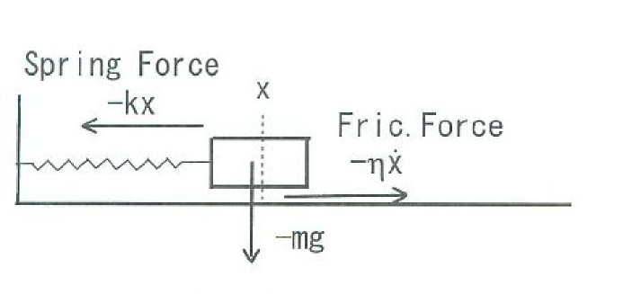
Figure 2: The harmonic oscillator with friction, (58).

6 Classical and Quantum Mechanics and Its Trajectory Geometry

We can treat the classical mechanics and its quantization ( the quantum mechanics, not the quantum field theory) in the same way. In this case, the model is simpler than the previous case (space-field theory) and we can see the geometrical structure clearly. Let us begin with the energy function of a system variable , $x$, (1 degree of freedom). For example the position (in 1 dimensional space) of the harmonic oscillator with friction. We take the following $n$-th energy function to define the step flow.

$$K_{n}(x)=V(x)+\frac{\eta}{2h}(x-x_{n-1})^{2}+\frac{m}{2h^{2}}(x-2x_{n-1}+x_{n-2})^{2}+K_{n}^{0}{\quad,}$$ (56)

where $V(x)$ is the general potential and $K_{n}^{0}$ is a constant which does not depend on $x$. For the harmonic oscillator $V(x)=kx^{2}/2$ where $k$ is the spring constant. $\eta$ is the viscosity and $m$ is the particle mass. We assume $x_{n-1}$ and $x_{n-2}$ are given values. As in Sec.2, the n-th step position ${x_{n}}$ is given by the minimal principle of the n-th energy function $K_{n}(x)$: $\delta K_{n}=0,x\rightarrow x+\delta x$.

$$\left.\frac{\delta V}{\delta x}\right|_{x={x_{n}}}+\frac{\eta}{h}({x_{n}}-x_{n-1})+\frac{m}{h^{2}}({x_{n}}-2x_{n-1}+x_{n-2})=0{\quad,}$$ (57)

This is the recursion relation among three quantities, $x_{n}$, $x_{n-1}$ and $x_{n-2}$. With the time $t_{n}$ (6), the continuous limit ($h\rightarrow 0$) gives us

$$\frac{dV(x)}{dx}+\eta\frac{dx}{dt}+m\frac{d^{2}x}{dt^{2}}=0{\quad,}$$ (58)

where $t_{n}=nh\rightarrow t,\ {x_{n}}=x(t_{n})\rightarrow x(t),\ ({x_{n}}-x_{n-1})/h=dx/dt|_{t_{n}}\rightarrow dx/dt,\ ({x_{n}}-2x_{n-1}+x_{n-2})/h^{2}=d^{2}x/dt^{2}|_{t_{n}}\rightarrow d^{2}x/dt^{2}\$. For the case of $V=kx^{2}/2$, this is the harmonic oscillator with the friction  $\eta$. See Fig.2. This is a simple dissipative system.

The recursion relation (57) gives us, for the initial data $x_{0}$ and $x_{1}$, the series {${x_{n}}=x(t_{n})\leavevmode\nobreak\ |n=0,1,2,\cdots$ }. This is the classical ’path’. The fluctuation of the path comes from the uncertainty principle of the quantum mechanics in this case. (We are treating the system of 1 degree of freedom. No statistical procedure is necessary. ) In the quantum effect, the energy uncertainty grows as $\Delta t\cdot\Delta E\geq\hbar$. Hence the path ${x_{n}}$, obtained by the recursion relation (57), has quantum uncertainty. As in Sec.4, we can generalize the n-th energy function $K_{n}(x)$, (56), to the following one $\Gamma(x_{n-1},x_{n-2})$ in order to take into account the quantum effect.

$${\rm e}^{-\frac{1}{\hbar}h\Gamma(x_{n-1},x_{n-2})}=\int_{-\infty}^{\infty}dx\leavevmode\nobreak\ {\rm e}^{-\frac{1}{\hbar}hK_{n}(x)}{\quad,}$$

$$K_{n}(x)=V(x)+\frac{\eta}{2h}(x-x_{n-1})^{2}+\frac{m}{2h^{2}}(x-2x_{n-1}+x_{n-2})^{2}+K_{n}^{0}{\quad.}$$ (59)

We can evaluate the quantum effect by the expansion around the classical value ${x_{n}}$ : $x={x_{n}}+\sqrt{\hbar}\leavevmode\nobreak\ q$ where $\hbar$ is Planck constant.

$${\rm e}^{-\frac{1}{\hbar}h\Gamma({x_{n}};x_{n-1},x_{n-2})}=\int dx\leavevmode\nobreak\ {\rm e}^{-\frac{1}{\hbar}hK_{n}(x)}=\int dq\leavevmode\nobreak\ {\rm e}^{-\frac{1}{\hbar}hK_{n}({x_{n}}+\sqrt{\hbar}q)}{\quad,}$$

$$\left.\frac{\delta K_{n}}{\delta x}\right|_{x={x_{n}}}=\left.\frac{\delta V}{\delta x}\right|_{x={x_{n}}}+\frac{\eta}{h}({x_{n}}-x_{n-1})+\frac{m}{h^{2}}({x_{n}}-2x_{n-1}+x_{n-2})=0{\quad,}$$

$$\Gamma_{n}\equiv\Gamma({x_{n}};x_{n-1},x_{n-2})=K_{n}({x_{n}})+\frac{\hbar}{2h}\ln(k+\frac{\eta}{h}+\frac{m}{h^{2}}){\quad,}$$ (60)

where the final expression is for the oscillator model: $V=kx^{2}/2$. The quantum effect does not depend on the step number $n$. It means the quantum effect contributes to the energy as an additional fixed constant at each step.

The energy rate is obtained as

$$h\frac{dK({t_{n}})}{d{t_{n}}}\equiv K_{n+1}(x_{n+1})-K_{n}(x_{n})=\Gamma_{n+1}-\Gamma_{n}\equiv h\frac{d\Gamma({t_{n}})}{d{t_{n}}}$$

$$=V(x_{n+1})-V({x_{n}})+\frac{\eta}{2h}\{(x_{n+1}-x_{n})^{2}-(x_{n}-x_{n-1})^{2}\}$$

$$+\frac{m}{2h^{2}}\{(x_{n+1}-2x_{n}+x_{n-1})^{2}-(x_{n}-2x_{n-1}+x_{n-2})^{2}\}K_{n+1}^{0}-K_{n}^{0}{\quad.}$$ (61)

The present system is again an open system, and the energy generally changes.

In terms of the position difference ${x_{n}}-x_{n-1}\equiv\Delta x_{n}$ and the velocity difference $({x_{n}}-2x_{n-1}+x_{n-2})/h\equiv v_{n}-v_{n-1}\equiv\Delta v_{n}$, we can rewrite the energy at $n$-step and read the metric as follows.

$$K_{n}({x_{n}})=V({x_{n}})+\frac{\eta}{2h}({x_{n}}-x_{n-1})^{2}+\frac{m}{2h^{2}}({x_{n}}-2x_{n-1}+x_{n-2})^{2}+K_{n}^{0}$$

$$=\frac{1}{h^{2}}\{V({x_{n}})(\Delta t)^{2}+\frac{\eta h}{2}(\Delta{x_{n}})^{2}+\frac{mh^{2}}{2}(\Delta v_{n})^{2}\}+K_{n}^{0}{\quad,}$$ (62)

where $h$ (time increment) in the first term within the round brackets is replaced by $\Delta t$. This shows us the metric for the n-step energy function is given by

$$(\Delta s_{n})^{2}\equiv 2h^{2}(K_{n}({x_{n}})-K_{n}^{0})=2V({x_{n}}^{\prime}/\sqrt{\eta h})(\Delta t)^{2}+(\Delta{x_{n}}^{\prime})^{2}+(\Delta v_{n}^{\prime})^{2}{\quad,}$$

$${x_{n}}^{\prime}\equiv\sqrt{\eta h}{x_{n}}{\quad,}\quad{v_{n}}^{\prime}\equiv\sqrt{mh^{2}}v_{n}{\quad,}$$ (63)

where , for the oscillator model, $V({x_{n}}^{\prime}/\sqrt{\eta h})=(k^{\prime}/2){{x_{n}}^{\prime}}^{2},k^{\prime}\equiv k/\eta h$. Eq.(63) shows the energy-line element ${\Delta s}^{2}$ in the ($t,{x_{n}}^{\prime},{v_{n}}^{\prime}$) space. Note that the above metric is along the path $x_{n}=x(t_{n}),\ v_{n}=v(t_{n})=(x(t_{n})-x(t_{n-1}))/h$ given by (57). The metric is used, in the next section, as the geometrical basis for fixing the statistical ensemble.

We define the system energy SysE_n, the dissipative energy DisE_n and the constant $K_{n}^{0}$ as follows.

$$\mbox{\text@underline{SysE}}_{n}=\frac{1}{m}V({x_{n}})+\frac{1}{2h^{2}}({x_{n}}-2x_{n-1}+x_{n-2})^{2}{\quad,}\quad\mbox{\text@underline{DisE}}_{n}=\frac{\eta}{2hm}({x_{n}}-x_{n-1})^{2}{\quad,}$$

$$K_{n}^{0}=0{\quad,}\quad K_{n}({x_{n}})=m\mbox{\text@underline{SysE}}_{n}+m\mbox{\text@underline{DisE}}_{n}{\quad.}$$ (64)

DisE_n expresses the hysteresis (non-Markovian) energy at the n-th step. We can obtain the dynamical energy (the potential energy plus the kinetic energy) DynE_n as

$${\mbox{\text@underline{DynE}}}_{n}=\frac{1}{m}V({x_{n}})+\frac{1}{2h^{2}}({x_{n}}-x_{n-1})^{2}{\quad.}$$ (65)

For the special case of the following, we list the simulation results here and in App.C. The horizontal axis is $t_{n}\omega=nh\omega$.

$$h=0.1{\quad,}\quad\omega=\sqrt{k/m}=0.01{\quad,}\quad\eta^{\prime}=\eta/m=0.005(\mbox{Elasticity dominate}){\quad,}$$

$$0\leq t_{n}\omega=nh\omega\leq 20{\quad,}\quad\mbox{total step no}=20000.{\quad.}$$ (66)

The movement $x_{n}$ and the velocity distribution $v_{n}=(x_{n}-x_{n-1})/h$ are shown in App.C. The dissipative energy DisE_n and the system energy SysE_n are shown in Fig.3 and Fig.4 respectively. They are , in the oscillatory way, damping. The dynamical energy DynE_n is shown in Fig.5. It damps, not in the oscillatory way but in the stick-slip way.

An advantageous point of the step-wise solution (57) over the analytic one of (58), is that we need not treat the 3 cases, $4k/m\leavevmode\nobreak\ >\leavevmode\nobreak\ \eta^{2}/m^{2}$ (elasticity dominate), $4k/m\leavevmode\nobreak\ <\leavevmode\nobreak\ \eta^{2}/m^{2}$ (viscosity dominate) and $4k/m\leavevmode\nobreak\ =\leavevmode\nobreak\ \eta^{2}/m^{2}$ (resonant), separately. This is because (57) is linear with repect to (w.r.t.) $x_{n}$, whereas (58) is the second-order equation w.r.t. $d/dt$.

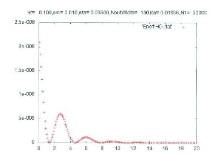
Figure 3: The dissipative energy DisE_n, (64), of the frictional harmonic oscillator Fig.2 with the parameters (66) .

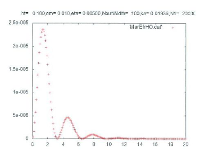
Figure 4: The system energy SysE_n, (64), of the frictional harmonic oscillator Fig.2 with the parameters (66) .

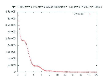
Figure 5: The dynamical energy DynE_n, (65), of the frictional harmonic oscillator Fig.2 with the parameters (66) .

7 Statistical Ensemble, Geometry and Initial Condition

In this section, we consider a statistical ensemble of the classical mechanical system taken in the previous section. Namely, we take $N$ ’copies’ of the classical model and regard them as a set of (1 dimensional) particles, where the dynamical configuration distributes in the probabilistic way. $N$ is a large number. The set has $N$ degrees of freedom: $x_{1},x_{2},\cdots,x_{N}$. As the physical systems, (1 dimensional) viscous gas and viscous liquid are examples. Each particle obeys the (step-wise) Newton’s law (57) with different initial conditions. $N$ is so large that we do not or can not observe the initial data. Usually we do not have interest in the trajectory of every particle and do not observe it. We have interest only in the macroscopic quantities such as total energy and total entropy. The N particles (fluid molecules) in the present system are ”moderately” interacting each other in such a way that each particle almost independently moves except that energy is exchanged.

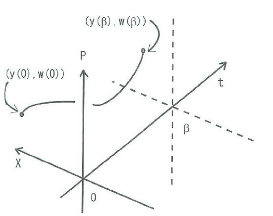
Figure 6: The path $\{(y(t),w(t),t)|0\leq t\leq\beta\}$ of line in 3D bulk space (X,P,t).

As the statistical ensemble, we adopt the Feynman’s idea of ”path-integral” [21, 22, 23, 24, 25, 26, 20, 19]. We take into account all possible paths $\{y_{n}\}$. $\{y_{n}\}$ need not satisfy (57) nor certain initial condition. As the measure for the summation (integral) over all paths, we propose the following ones based on the geometry of (63). As the first measure, we construct it in terms of the length, using the ”Dirac-type” metric [20, 19].

$$(ds^{2})_{D}\equiv 2V(X)dt^{2}+dX^{2}+dP^{2}\quad-\mbox{on-path}(X=y(t),P=w(t))\rightarrow$$

$$(2V(y)+\dot{y}^{2}+\dot{w}^{2})dt^{2}{\quad,}$$

$$L_{D}=\int_{0}^{\beta}ds|_{on-path}=\int_{0}^{\beta}\sqrt{2V(y)+\dot{y}^{2}+\dot{w}^{2}}dt=h\sum_{n=0}^{\beta/h}\sqrt{2V(y_{n})+\dot{y}_{n}^{2}+\dot{w}_{n}^{2}}{\quad,}$$

$$d\mu={\rm e}^{-{\frac{1}{\alpha}}L_{D}}{\cal D}y{\cal D}w{\quad,}\quad{\rm e}^{-\beta F}=\int\prod_{n}dy_{n}dw_{n}{\rm e}^{-{\frac{1}{\alpha}}L_{D}}{\quad,}$$ (67)

where $\alpha$ is a parameter with the dimension of length ([$\alpha$]=L) and $V(X)=(k/2)X^{2}$. See Fig.6. As explained in Sec.4, it is appropriately chosen problem by problem. $\beta$ is introduced to restrict the $t$-region ($0\leq t\leq\beta$) and, in this context, should be regarded as a part of the choice of the ensemble. $\beta$ plays the role of the inverse temperature. Among all possible paths $\{y_{n}\}$, the minimal length ($\delta L_{D}=0$) solution, (57), gives the dominant path $\{x_{n}\}$.

The second choice is constructed using the ”Standard-type” metric.

$$(ds^{2})_{S}\equiv\frac{1}{dt^{2}}[(ds^{2})_{D}]^{2}\quad-\mbox{on-path}(X=y(t),P=w(t))\rightarrow$$

$$(2V(y)+\dot{y}^{2}+\dot{w}^{2})^{2}dt^{2}{\quad,}$$

$$L_{S}=\int_{0}^{\beta}ds|_{on-path}=\int_{0}^{\beta}(2V(y)+\dot{y}^{2}+\dot{w}^{2})dt=h\sum_{n=0}^{\beta/h}(2V(y_{n})+\dot{y}_{n}^{2}+\dot{w}_{n}^{2}){\quad,}$$

$$d\mu={\rm e}^{-{\frac{1}{\alpha}}L_{S}}{\cal D}y{\cal D}w\ ,\ {\rm e}^{-\beta F}=\int\prod_{n}dy_{n}dw_{n}{\rm e}^{-{\frac{1}{\alpha}}L_{S}}=(\mbox{const})\int\prod_{n}dy_{n}{\rm e}^{-\frac{h}{\alpha}(2V(y_{n})+\dot{y}_{n}^{2})}\ ,$$ (68)

where we should notice $dt$ ($=h>0$) is non-zero. In both cases above we take the metric of the 3 dimensional (bulk) space-time (X, P, t) , which is consistently chosen with the trajectory metric (63). Note that the standard case has the same expression as the free energy (trace of the density matrix) expression in the Feynman’s textbook[27].

Figure 7: The two dimensional surface, (69), in 3D bulk space (X,P,t).

Another choice of path is making use of surfaces instead of lines. Let us consider the following 2 dim surface in the 3 dim manifold ($X,P,t$). Assuming Z₂ invariance both in $X$ and in $P$, the general one is

$$\frac{X^{2}}{a(t)^{2}}+\frac{P^{2}}{b(t)^{2}}=1{\quad,}\quad 0\leq t\leq\beta{\quad,}$$ (69)

where $a(t)$ and $b(t)$ are arbitrary (positive) functions of $t$. We take $a(t)=b(t)\equiv r(t)$ for simplicity. See Fig.7. By varying the form of $\{r(t):\ 0\leq t\leq\beta\}$, we obtain different surfaces. Regarding each of them as a path used in the Feynman’s path-integral, we obtain the following statistical ensemble. First the induced metric $g_{ij}$ on the surface (69) is given as

$$\left.(ds^{2})_{D}\right|_{\mbox{on-path}}=\left.2V(X)dt^{2}+dX^{2}+dP^{2}\right|_{\mbox{on-path}}=\sum_{i,j=1}^{2}g_{ij}dX^{i}dX^{j}{\quad,}$$

$$(g_{ij})=\left(\begin{array}[]{cc}1+\frac{2V}{r^{2}\dot{r}^{2}}X^{2}&\frac{2V}{r^{2}\dot{r}^{2}}XP\\ \frac{2V}{r^{2}\dot{r}^{2}}PX&1+\frac{2V}{r^{2}\dot{r}^{2}}P^{2}\end{array}\right){\quad,}$$ (72)

where $(X^{1},X^{2})=(X,P)$. Then the area of the surface (69) is given by

$$A=\int\sqrt{\det g_{ij}}d^{2}X=\int\sqrt{1+\frac{2V}{\dot{r}^{2}}}dXdP{\quad.}$$ (73)

We consider all possible surfaces of (69). The statistical distribution is, using the area $A$, given by

$${\rm e}^{-\beta F}=\int_{0}^{\infty}d\rho\int_{\begin{array}[]{c}r(0)=\rho\\ r(\beta)=\rho\end{array}}\prod_{t}{\cal D}X(t){\cal D}P(t){\rm e}^{-\frac{1}{\alpha}A}{\quad.}$$ (76)

In relation to Boltzmann’s equation (Sec.5), we have directly defined the distribution function $f(t,x,v)$ using the geometrical quantities in the 3 dim bulk space. Three statistical ensembles are proposed. In order to select which one is the most appropriate, it is necessary to numerically evaluate the models with the proposed ensembles and compare the result with the real data appearing both in the natural phenomena and in the laboratory experiment.

In App.D, another model called ”Spring-Block” model is explained. This is the simplified model of the earthquake. The same thing in this section is valid by taking the potential $V(X)$ as

$$V(X)=\frac{k^{\prime}}{2}X^{2}+(\bar{l}^{\prime}-{\bar{V}}^{\prime}t)k^{\prime}X\ ,\ k^{\prime}=\frac{k}{\eta h}\ ,\ \bar{l}^{\prime}=\sqrt{\eta h}\bar{l}\ ,\ {\bar{V}}^{\prime}=\sqrt{\eta h}{\bar{V}}\ .$$ (77)

8 Conclusion

We have presented the field theory approach to Boltzmann’s transport equation. The collision term is explicitly obtained. Time is not used, instead the step number $n$ plays the role. We have presented the $n$-th energy functional (10) which gives the step $n$ configuration ${u_{n}}(x)$ from the minimal energy principle. We regard the step flow ( the increase of $n$ ) as the evolution of the system, namely, time-development. Burgers (Navier-Stokes) equation is obtained by identifying time $t$ as $nh$ (6). Fluctuation effect due to the micro structure and micro (step-wise) movement is taken into account by generalizing the $n$-th energy functional ${\tilde{I}}_{n}[u(x)]$, (10), to $\Gamma[u(x);u_{n-1}(x)]$, (27), where the classical path ${u_{n}}(x)$ is dominant but all possible paths are taken into account (path-integral). Renormalization, due to the statistical fluctuation, is explicitly done. The total energy generally does not conserve. The system is an open one, namely, the energy comes in from or go out to the outside. In the latter part of the text, we have presented a direct approach to the distribution function $f_{n}(x,v)$ based on the geometry emerging from the mechanical (particle-orbit) dynamics. We have examined the dissipative system using the minimal (variational) principle which is the key principle in the standard field theory[28].

9 Appendix A  (3+1)D Scalar Field Theory

3+1 dimensional scalar field is here treated in the present step-wise formalism. We start with the following $n$-th step energy functional.

$$I_{n}[\phi({\bf x})]={\int d^{3}x}\{\frac{1}{2}({{\bf\nabla}}\phi)^{2}+V(\phi)+\frac{1}{2h^{2}}(\phi-2\phi_{n-1}+\phi_{n-2})^{2}\}\quad n=2,3,\cdots{\quad,}$$

$$V(\phi)=\frac{m^{2}}{2}\phi^{2}+\frac{\lambda}{4!}\phi^{4}{\quad,}\quad\phi=\phi({\bf x})\ ,\ \phi_{n-1}=\phi_{n-1}({\bf x}),\ \phi_{n-2}=\phi_{n-2}({\bf x}){\quad,}$$ (78)

where $\phi_{n-2}$ and $\phi_{n-1}$ are given. $({\bf x})=(x_{1},x_{2},x_{3})$ is the 3 dimensional spacial coordinates. The step $n$ configuration ${\phi_{n}}({\bf x})$ is defined to be the energy minimal one.

$$\left.\frac{\delta I_{n}}{\delta\phi}\right|_{\phi={\phi_{n}}}=-{{\bf\nabla}}^{2}{\phi_{n}}+\left.\frac{\delta V}{\delta\phi}\right|_{\phi={\phi_{n}}}+\frac{1}{h^{2}}({\phi_{n}}-2\phi_{n-1}+\phi_{n-2})=0{\quad,}$$

$$\frac{\delta V}{\delta\phi}=m^{2}\phi+\frac{\lambda}{3!}\phi^{3}{\quad.}$$ (79)

Using the step-time notation: ${\phi_{n}}({\bf x})\equiv\phi({\bf x},{t_{n}}),\ {t_{n}}=nh$, we obtain, in the continuous time limit $h\rightarrow+0$,

$$(\partial_{t}^{2}-{\bf\nabla}^{2}+m^{2})\phi+\frac{\lambda}{3!}\phi^{3}=0{\quad.}$$ (80)

This is the (3+1) dim $\phi^{4}$ scalar field equation.

10 Appendix B  Calculation of Fluctuation Effect

In Sec.4, we have developed the method of calculating the statistical fluctuation occurring in the (1-dim) viscous fluid matter. The background-field method is taken. At the 1-loop approximation, the key quantity to calculate the energy functional $\Gamma[u(x)]$ is the heat-kernel $G(x,y;\tau)$ given by (see eq.(32))

$$<x|{\rm e}^{-\tau D}|y>\equiv G(x,y;\tau){\quad,}$$

$$(\frac{\partial}{\partial\tau}+D)G(x,y;\tau)=0{\quad,}\quad\lim_{\tau\rightarrow+0}G(x,y;\tau)=\delta(x-y){\quad,}$$

$$D=-\epsilon^{-1}\frac{\partial^{2}}{\partial x^{2}}+2u_{n-1}(x)A\frac{d}{dx}-{\bar{V}}(x){\quad,}\quad{\bar{V}}(x)=-\lambda{u_{n}(x)}^{2}-m^{2}-\frac{1}{h}{\quad,}$$ (81)

where $|x>$ and $<x|$ are Dirac’s abstract state vectors. $\epsilon\equiv{\tilde{\rho}}_{0}/\sigma$ is explicitly written to show the dimension consistency. We take $A=0$ in this appendix. In the text, we take $\epsilon=1$. For the calculation, in this appendix, we change the scale of $\tau$ and $D$ as follows.

$$\tau\quad\rightarrow\quad\frac{\tau}{\epsilon}={\tilde{\tau}}{\quad,}\quad D\quad\rightarrow\quad\epsilon D={\tilde{D}}{\quad,}$$

$${\tilde{D}}=-\frac{\partial^{2}}{\partial x^{2}}-\epsilon{\bar{V}}(x){\quad,}\quad\mbox{[${\tilde{\tau}}$]=L${}^{2}$}{\quad,}\quad\mbox{[${\tilde{D}}$]=L${}^{-2}$}{\quad,}\quad\mbox{[$\epsilon$]=1/LM}{\quad.}$$ (82)

In the following within this appendix, for simplicity we omit the symbol of ’tilde’.

The kernel is formally solved as

$$G(x,y;\tau)=G_{0}(x-y;\tau)+\int dz\int_{0}^{\tau}d\omega S(x-z;\tau-\omega)\epsilon{\bar{V}}(z)G(z,y;\omega){\quad,}$$ (83)

where $G_{0}(x-y;\tau)$ and the (heat-)propagator $S(x-y;\tau)$ are given by

$$G_{0}(x-y;\tau)=\int_{-\infty}^{\infty}\frac{dk}{2\pi}{\rm e}^{-k^{2}\tau+ik(x-y)}=\frac{1}{\sqrt{4\pi\tau}}{\rm e}^{-\frac{(x-y)^{2}}{4\tau}}{\quad,}\quad\tau>0{\quad,}$$

$$S(x-y;\tau)=\int\int_{-\infty}^{\infty}\frac{dk}{2\pi}\frac{dk^{0}}{2\pi}\frac{\exp\{-ik^{0}\tau+ik(x-y)\}}{-ik^{0}+k^{2}}=\theta(\tau)G_{0}(x-y;\tau){\quad.}$$ (84)

They satisfy

$$(\frac{\partial}{\partial\tau}-\frac{\partial^{2}}{\partial x^{2}})G_{0}(x-y;\tau)=0{\quad,}\quad\tau>0{\quad,}\quad\lim_{\tau\rightarrow+0}G_{0}(x-y;\tau)=\delta(x-y){\quad,}$$

$$(\frac{\partial}{\partial\tau}-\frac{\partial^{2}}{\partial x^{2}})S(x-y;\tau)=\delta(\tau)\delta(x-y){\quad,}\quad\lim_{\tau\rightarrow+0}S(x-y;\tau)=\delta(x-y){\quad.}$$ (85)

Up to the first order of ${\bar{V}}$,

$$G(x,x;\tau)=\frac{1}{\sqrt{4\pi\tau}}+\int dz\int_{0}^{\tau}d\omega S(x-z;\tau-\omega)\epsilon{\bar{V}}(z)G_{0}(z-x;\omega)+O({\bar{V}}^{2}){\quad.}$$ (86)

The second term is evaluated as

$$\int dz\int_{0}^{\tau}d\omega G_{0}(x-z;\tau-\omega)\epsilon{\bar{V}}(z)G_{0}(z-x;\omega)=$$

$$\int dz\int_{0}^{\tau}d\omega\frac{1}{4\pi}\frac{1}{\sqrt{(\tau-\omega)\omega}}\epsilon{\bar{V}}(z)\exp\{-\frac{\tau}{4(\tau-\omega)\omega}(x-z)^{2}\}{\quad.}$$ (87)

Finally the contribution to $\ln(\det D)^{-1/2}={1\over 2}\int_{0}^{\infty}(d\tau/\tau){\rm Tr}G(x,y;\tau)=$
${1\over 2}\int_{0}^{\infty}(d\tau/\tau)\int_{-l}^{l}dxG(x,x;\tau)$ is evaluated as

$${1\over 2}\int_{0}^{\infty}d\tau{1\over 2}\frac{1}{\sqrt{\tau\pi}}\int dz\epsilon{\bar{V}}(z)=\frac{1}{4\sqrt{\pi}}\int_{0}^{\epsilon^{-1}\mu^{-1}}\tau^{-1/2}d\tau\int dz\epsilon{\bar{V}}(z)=$$

$$\frac{l}{\sqrt{\pi}}\sqrt{\epsilon\Lambda}-\frac{1}{2\sqrt{\pi\epsilon\mu}}\int_{-l}^{l}dz\epsilon\left(\lambda{u_{n}}(z)^{2}+m^{2}+\frac{1}{h}\right){\quad,}$$ (88)

where the infrared cut-off parameter $\mu\equiv\sqrt{\sigma}/l$ and the ultraviolet cut-off parameter $\Lambda\equiv h^{-1}$ are introduced.

11 Appendix C  Simulation of Frictional Harmonic Oscillator

In Sec.6, we take the frictional harmonic model Fig.2. Some simulation results (Fig.3, Fig.4, Fig.5) are shown there. In this appendix, we show additional results.

The step-wise solution (57), $x_{n}$, is shown in Fig.8. It reproduces the analytic solution.

$$x(t)={\rm e}^{-\eta^{\prime}t/2}\sin(\sqrt{4\omega^{2}-{\eta^{\prime}}^{2}}\leavevmode\nobreak\ t/2){\quad,}$$

$$0\leq t\leq 2000{\quad,}\quad x(0)=0{\quad,}\quad\dot{x}(0)=\sqrt{4\omega^{2}-{\eta^{\prime}}^{2}}/2=(1.94\times 10^{-2})/2{\quad.}$$ (89)

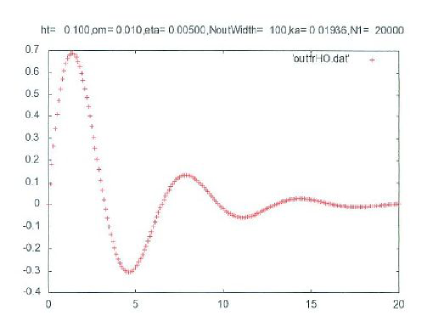
Figure 8: The movement $x_{n}$, (57), of the frictional harmonic oscillator Fig.2 with the parameters (66) (Elasticity dominate). The step-wise solution reproduces the analytic solution (89).

The velocity $v_{n}=(x_{n}-x_{n-1})/h$ is shown in Fig.9.

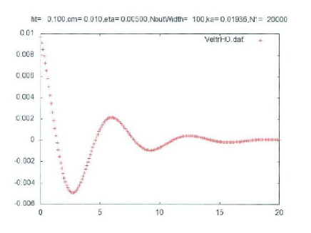
Figure 9: The velocity $v_{n}=(x_{n}-x_{n-1})/h$ of the frictional harmonic oscillator Fig.2 with the parameters (66) (Elasticity dominate).

The sum of the system energy SysE_n (Fig.4) and the dissipative energy DisE_n (Fig.3) is shown in Fig.10.

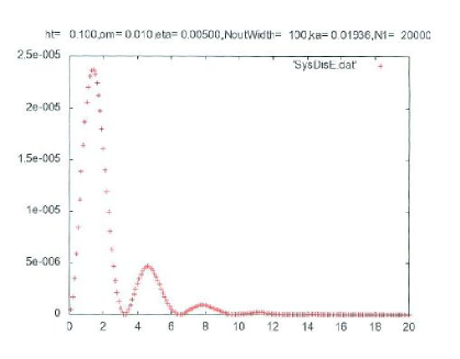
Figure 10: The system energy (SysE_n, Fig.4) plus the dissipative energy (DisE_n, Fig.3) of the frictional harmonic oscillator Fig.2 with the parameters (66) (Elasticity dominate).

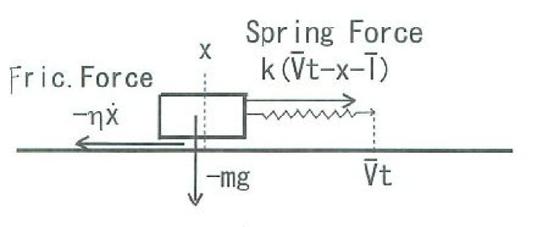
Figure 11: The spring-block model, (92).

12 Appendix D  Spring-Block Model

In Sec.6, the movement of the harmonic oscillator with friction was examined. Here we treat the movement of a block which is pulled by the spring which moves at the constant speed ${\bar{V}}$. See Fig.11. The block moves on the surface with friction. We take the following $n$-th energy function to define the step flow.

$$K_{n}(x)=V(x)-hnk{\bar{V}}x+\frac{m}{2h^{2}}(x-2x_{n-1}+x_{n-2})^{2}+\frac{\eta}{2h}(x-x_{n-1})^{2}+K_{n}^{0}{\quad,}$$

$$V(x)=\frac{kx^{2}}{2}+k\bar{l}x{\quad,}$$ (90)

where $\eta$ is the friction coefficient and $m$ is the block mass. The potential $V(x)$ has two terms: one is the harmonic oscillator with the spring constant $k$, and the other is the linear term of x with a new parameter $\bar{l}$ (the natural length of the spring). ${\bar{V}}$ is the velocity (constant) with which the front-end of the spring moves. $K_{n}^{0}$ is a constant which does not depend on $x$. It will be fixed later. The $n$-th step ${x_{n}}$ is determined by the energy minimum principle: $\delta K_{n}(x)|_{x={x_{n}}}=0$.

$$\frac{k}{m}({x_{n}}+\bar{l}-nh{\bar{V}})+\frac{\eta}{m}\frac{1}{h}({x_{n}}-x_{n-1})+\frac{1}{h^{2}}({x_{n}}-2x_{n-1}+x_{n-2})=0\quad\mbox{or}$$

$${x_{n}}=\frac{\omega^{2}(-\bar{l}+nh{\bar{V}})+\frac{{\eta^{\prime}}}{h}x_{n-1}+\frac{1}{h^{2}}(2x_{n-1}-x_{n-2})}{\omega^{2}+\frac{\eta^{\prime}}{h}+\frac{1}{h^{2}}},\ \omega\equiv\sqrt{\frac{k}{m}}\ ,\ {\eta^{\prime}}\equiv\frac{\eta}{m}{\quad.}$$ (91)

For the continuous limit: $h\rightarrow 0,nh=t_{n}\rightarrow t,({x_{n}}-x_{n-1})/h\rightarrow\dot{x},({x_{n}}-2x_{n-1}+x_{n-2})/h^{2}\rightarrow\ddot{x}$, the above recursion relation reduces to the following differential equation.

$$m\ddot{x}=k({\bar{V}}t-x-\bar{l})-\eta\dot{x}{\quad.}$$ (92)

We keep the step-wise approach. The system energy given by $K_{n}({x_{n}})$. Taking the constant term $K_{n}^{0}$ as

$$K_{n}^{0}=-V({x_{n}})-\frac{m}{2h^{2}}({x_{n}}-2x_{n-1}+x_{n-2})^{2}+hnk{\bar{V}}{x_{n}}+V(x_{0})+\frac{m}{2h^{2}}(x_{1}-x_{0})^{2},$$ (93)

the energy is given as

$$K_{n}({x_{n}})=\frac{\eta}{2h}({x_{n}}-x_{n-1})^{2}+V(x_{0})+\frac{m}{2h^{2}}(x_{1}-x_{0})^{2}{\quad,}$$ (94)

This is the same as (65). We have taken the constant term $K^{0}_{n}$, (93), in such a way that the system keeps the constant energy when the energy dissipation does not occur . The first three terms in (93) comes from the following relation derived from (92).

$$\left[\frac{m}{2}\dot{x}^{2}+\frac{k}{2}x^{2}+k\bar{l}x\right]_{0}^{t}+\left[-k{\bar{V}}xt\right]_{0}^{t}+\int_{0}^{t}(\eta\dot{x}^{2}+k{\bar{V}}x)dt=0{\quad.}$$ (95)

We use the equation : $\int_{0}^{t}(-k{\bar{V}}\dot{x}t)dt=\left[-k{\bar{V}}xt\right]_{0}^{t}+\int_{0}^{t}(k{\bar{V}}x)dt$. The terms bracketed above correspond to the first three terms in $K_{n}(x_{n})$ which is obtained by taking $x=x_{n}$ in (90). Those terms are regarded as Markovian and canceled by the first three terms in (93).

The graphs of movement (${x_{n}}$, eq.(91)) and energy change ($K_{n}({x_{n}})$, eq.(94)) are shown in Fig.12 and Fig.14 respectively. The velocity change ($v_{n}\equiv(x_{n}-x_{n-1})/h$) is also shown in Fig.13. From the graphs, we see this system does the stick-slip motion. The stick regions correspond to the neighbor of the local minimums in the velocity change Fig.13. The system oscillates periodically in the velocity (Fig.13) and in the energy (Fig.14). The oscillation amplitudes decay as the step goes (relaxation). Finally the system reaches the steady energy-state as $n\rightarrow\infty$, (26).

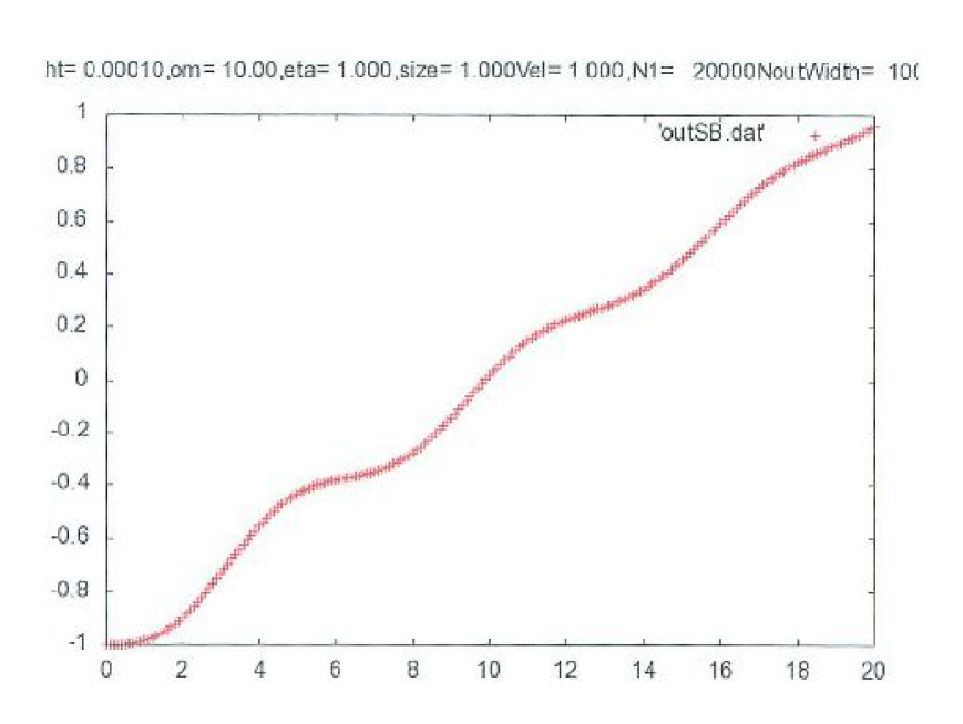
Figure 12: Spring-Block Model, Movement (91), $h$=0.0001,$\omega=\sqrt{k/m}$=10.0, $\eta^{\prime}=\eta/m$=1.0, ${\bar{V}}$=1.0, $\bar{l}$=1.0, total step no =20000. The horizontal axis is $n\times h\times\omega$. The step-wise solution (91) correctly reproduces the analytic solution: $x(t)={\rm e}^{-\eta^{\prime}t/2}{\bar{V}}\{({\eta^{\prime}}^{2}/2\omega^{2}-1)(\sin\Omega t)/\Omega+(\eta^{\prime}/\omega^{2})\cos\Omega t\}-\bar{l}+{\bar{V}}(t-\eta^{\prime}/\omega^{2}){\quad,}\Omega=(1/2)\sqrt{4\omega^{2}-{\eta^{\prime}}^{2}}=9.99{\quad,}\ 0\leq t\leq 2{\quad,}\quad x(0)=-\bar{l},\ \dot{x}(0)=0$.

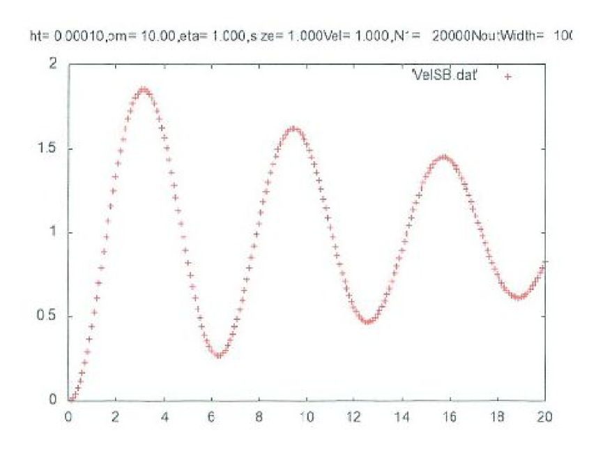
Figure 13: Velocity $(x_{n}-x_{n-1})/h\equiv v_{n}$, $h$=0.0001,$\omega=\sqrt{k/m}$=10.0, $\eta^{\prime}=\eta/m$=1.0, ${\bar{V}}$=1.0, $\bar{l}$=1.0, total step no =20000.

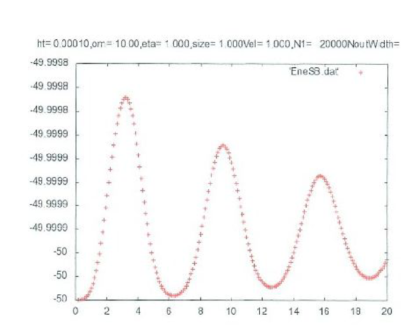
Figure 14: Spring-Block Model, Energy Change (94), $h$=0.0001,$\omega=\sqrt{k/m}$=10.0, $\eta^{\prime}=\eta/m$=1.0, ${\bar{V}}$=1.0, $\bar{l}$=1.0, total step no =20000.

13 Acknowledgment

This work has finished during the author’s stay in DAMTP, Cambridge. He thanks all members for the hospitality, especially G. W. Gibbons for comments about this work. He also thanks N. Kikuchi (Keio Univ., Japan) for introducing his theory[2]. The present research starts from it. Finally the author thanks K. Mori (Saitama Univ., Japan) for the continual advices about mathematics and physics which leads to this work. This research project is financially supported by University of Shizuoka. ( March 2013 )

The content is now improved and was reported in some workshops and conferences[30].

References

- [1] G. W. Gibbons, ”The emergent nature of time and the complex numbers in quantum cosmology”, The Arrows of Time, Fundamental Theories of Physics Vol.172, Houghton et al (eds.), pp 107-146, Springer 2012. arXiv: 1111.0457
- [2] N. Kikuchi, An approach to the construction of Morse flows for variational functionals in ”Nematics-Mathematical and Physical Aspects”, eds. J. -M. Coron, J. -M. Ghidaglia and Hélein, NATO Adv. Sci. Inst. Ser. C: Math. Phys. Sci. 332, Kluwer Acad. Pub., Dordrecht-Boston-London, 1991, p195-198
- [3] N. Kikuchi, A method of constructing Morse flows to variational functionals. Nonlin. World 131(1994)
- [4] L. Ma and I. Witt, arXiv: 1203.2225[math.DG] ”Discrete Morse flow for Ricci flow and porous media equation”
- [5] S. Succi, ”The Lattice Boltzmann Equation”, Oxford University Press Inc., New York, 2001
- [6] B. S. DeWitt, Phys. Rev. 162, 1195, 1239(1967)
- [7] G. ’t Hooft, Nucl.Phys.B62(1973)444
- [8] M. B. Green, J. H. Schwartz and E. Witten, Superstring theory, Vol.I and II, Cambridge Univ. Press, c1987, Cambridge
- [9] J. Polchinski, STRING THEORY, Vol.I and II, Cambridge Univ. Press, c1998, Cambridge
- [10] J.M. Maldacena, Adv.Theor.Math.Phys.2(1998)231 [Int. J. Theor. Phys.38(1999)1113], arXiv:hep-th/9711200
- [11] S. S. Gubser, I. R. Klebanov and A. M. Polyakov, Phys.Lett.B428(1998)105, arXiv:hep-th/9802109
- [12] E. Witten, Adv. Theor. Math. Phys.2(1998)253, arXiv:hep-th/9802150
- [13] M. Natsuume, AdS/CFT Duality User Guide (Lecture Notes in Physics), Springer, c2015
- [14] M. Ammon and J. Erdmenger, Gauge/Gravity Duality: Foundations and Applications, Cambridge University Press, c2015
- [15] M. Natsuume, Prog. Theor. Phys. Suppl. 174: 286(2008), arXiv:0807.1394[nucl-th]
- [16] J. Schwinger, Phys.Rev.82(1951)664
- [17] M.L. Bellac, F. Mortessagne and G.G. Batrouni, ”Equilibrium and Non-Equilibrium Statistical Thermodynamics”, Cambridge Univ. press, Cambridge, 2004
- [18] S. Weinberg, ”The Quantum Theory of Fields I”, Cambridge Univ. press, CambridgeNew YorkMelbourne, 1995, p499
- [19] S. Ichinose, J.Phys:Conf.Ser.258(2010)012003, arXiv:1010.5558, Proc. of Int. Conf. on Science of Friction 2010 (Ise-Shima, Mie, Japan, 2010.9.13-18).
- [20] S. Ichinose, arXiv:1004.2573, ”Geometric Approach to Quantum Statistical Mechanics and Minimal Area Principle”, 2010, 28 pages.
- [21] S. Ichinose, Prog.Theor.Phys.121(2009)727, ArXiv:0801.3064v8[hep-th].
- [22] S. Ichinose, ”Casimir Energy of 5D Warped System and Sphere Lattice Regularization”, ArXiv:0812.1263[hep-th], US-08-03, 61 pages.
- [23] S. Ichinose, ”Casimir Energy of AdS5 Electromagnetism and Cosmological Constant Problem”, Int.Jour.Mod.Phys.24A(2009)3620, Proc. of Int. Conf. on Particle Physics, Astrophysics and Quantum Field Theory: 75 Years since Solvay (Nov.27-29, 2008, Nanyang Executive Centre, Singapore), arXiv:0903.4971
- [24] S. Ichinose, J. Phys. : Conf.Ser.222(2010)012048. Proceedings of First Mediterranean Conference on Classical and Quantum Gravity (09.9.14-18, Kolymbari, Crete, Greece). ArXiv:1001.0222[hep-th]
- [25] S. Ichinose, ”New Regularization in Extra Dimensional Model and Renormalization Group Flow of the Cosmological Constant”, Proceedings of the Int. Workshop on ’Strong Coupling Gauge Theories in LHC Era’(09.12.8-11, Nagoya Univ., Nagoya, Japan) p407, eddited by H. Fukaya et al, World Scientific. ArXiv:1003.5041[hep-th]
- [26] S. Ichinose, J. Phys. : Conf.Ser.384(2012)012028, Proceedings of DSU2011 (2011.9.26-30, Beijin, China). ArXiv:1205.1316[hep-th]
- [27] R.P. Feynman, ”Statistical Mechanics”, W.A.Benjamin,Inc., Massachusetts, 1972
- [28] W. Yourgrau and S. Mandelstam, ”Variational Principles in Dynamics and Quantum Theory”, Dover Publications, Inc., New York, 1952, 1968, 1979
- [29] S. Ichinose, ”Non-equilibrium Statistical Approach to Friction Models”, Tribology International (Elsevier), in press. arXiv:1404.6627
- [30] S. Ichinose, JPS Conf.Proc. 1, 013103(2014), Proc. of the 12th Asia Pacific Phys. Conf., arXiv:1308.1238(hep-th)