Generalized Parton Distributions in the valence region from Deeply Virtual Compton Scattering

Abstract

This work reviews the recent developments in the field of Generalized Parton Distributions (GPDs) and Deeply virtual Compton scattering in the valence region, which aim at extracting the quark structure of the nucleon. We discuss the constraints which the present generation of measurements provide on GPDs, and examine several state-of-the-art parameterizations of GPDs. Future directions in this active field are discussed.

1 Introduction: PDFs, FFs and GPDs

1.1 PDFs, FFs and GPDs

Electron scattering, or more generally lepton scattering, has always been a powerful tool to investigate the structure of the subatomic world. This is due to the structureless nature of leptons and the way these latter interact with the target, i.e. mainly through the electromagnetic interaction which is described by an extremely precise theory: Quantum Electro-Dynamics (QED).

Since the late 60’s and the advent of electron accelerators in the GeV range, nucleon structure has been investigated by two main classes of electron scattering processes: inclusive scattering $eN\to e^{\prime}X$, also called “Deep Inelastic Scattering” (DIS), and elastic scattering $eN\to e^{\prime}N^{\prime}$, where $e$ ($e^{\prime}$) stand for an electron, or more generally a lepton, $N$ ($N^{\prime}$) for a nucleon and $X$ for an undefined final state.

We recall that Hofstadter was awarded the Nobel Prize in 1961 “for his pioneering studies of electron scattering in atomic nuclei” which revealed that the proton explicitly appeared as an extended object and not as a pointlike particle. These measurements have shown that as the momentum transfer increases in the elastic scattering, the cross section sharply decreases compared to the electron scattering on a pointlike charge. In contrast, for the inelastic scattering process it was found firstly at SLAC that the cross section at large momentum transfers does not show the sharp fall-off as elastic scattering but shows a scaling behavior. This so-called Bjorken scaling put in evidence the presence of pointlike charged constituents within the nucleons, for which the 1990 Nobel prize was awarded to Friedman, Kendall and Taylor. Through Feynman’s parton model, these consituents were then identified with the “quarks” introduced earlier by Gell-Mann (who was awarded the Nobel Prize in 1969 for his “Eightfold way”), based on theoretical symmetry considerations.

In a first approximation, electron scattering proceeds through a one-photon exchange (we will keep this approximation in the whole of this work) and is characterized by $Q^{2}=-(p_{e}-p_{e}^{\prime})^{2}>0$, the squared four-momentum transfered to the nucleon by the electron. The virtuality $Q^{2}$ of the spacelike virtual photon can be thought of as the resolution or the scale with which one probes the inner structure of the nucleon.

At sufficiently high $Q^{2}$, the quark structure of the nucleon can be “seen” and the DIS process can be depicted by Fig. 1 (left panel), where the incoming lepton interacts with a single quark of the nucleon via the exchange of a virtual photon. The signature of such a pointlike and elementary photon-quark process is the $Q^{2}$-independence of the amplitude of the process, i.e. the absence of a scale in the process. DIS results accumulated for more than 40 years show that this picture, so-called “scaling”, starts to be valid already at $Q^{2}\approx$ 1 GeV².

Figure 1: Left panel: Deep Inelastic Scattering: at high virtuality $Q^{2}$ of the photon exchanged between the electron and the nucleon, the photon interacts with a single quark of the nucleon. The struck quark escapes the nucleon and hadronizes leaving the final hadronic state undetermined. Right panel: Illustration of the associated non-local diagonal matrix element $\langle p|\bar{\psi}_{q}(0)\mathcal{O}\psi_{q}(y)|p\rangle$ accessed in DIS.

The complex quark and gluon structure of the nucleon, governed by the theory of strong interactions, Quantum Chromo-Dynamics (QCD), in its non-perturbative regime is then absorbed in structure functions. This is the concept of QCD factorization where one separates a point-like, short-distance, “hard” subprocess, from the complex, long-distance, “soft” structure of the nucleon. The calculation of such soft matrix elements directly from the underlying theory amounts to solve QCD in its non-perturbative regime, which is still a daunting task. Ab initio calculations, by evaluating QCD numerically on a discretized space-time euclidean lattice, are at present the most promising avenue to provide predictions for some category of such non-perturbative objects. In the DIS process, the soft structure functions are the well-known unpolarized and polarized Parton Distribution Functions (PDFs) $q(x)$ and $\Delta q(x)$ respectively. In a frame where the nucleon approaches the speed of light in a certain direction, $x$ is the longitudinal momentum fraction carried by the quark which is struck by the virtual photon. The PDFs represent therefore the (longitudinal) momentum distribution of quarks in the nucleon.

The PDF structure functions correspond to QCD operators depending on space-time coordinates. Precisely, the PDFs are obtained as one-dimensional Fourier transforms in the lightlike coordinate $y^{-}$ (at zero values of the other coordinates) as :

$$q(x)\, = \,{{p^{+}}\over{4\pi}}\,\int dy^{-}e^{ixp^{+}y^{-}}\langle p|\bar{\psi}_{q}(0)\gamma^{+}\psi_{q}(y)|p\rangle{\Bigg{|}}_{y^{+}=\vec{y}_{\perp}=0}\;,$$

$$\Delta q(x)\, = \,{{p^{+}}\over{4\pi}}\,\int dy^{-}e^{ixp^{+}y^{-}}\langle pS_{\|}|\bar{\psi}_{q}(0)\gamma^{+}\gamma_{5}\psi_{q}(y)|pS_{\|}\rangle{\Bigg{|}}_{y^{+}=\vec{y}_{\perp}=0}\;,$$ (1)

where $\psi_{q}$ is the quark field of flavor $q$, $p$ represents the initial (and final, since it is the same for DIS by virtue of the optical theorem) nucleon momentum, $x$ is the momentum fraction of the struck quark and $S_{\|}$ is the longitudinal nucleon spin projection.

One uses here the light-front frame where the initial and final nucleons are collinear along the $z$-axis and the light-cone components are defined by $a^{\pm}\equiv(a^{0}\pm a^{3})/\sqrt{2}$. Since the space-time coordinates of the initial and final quarks are different, the operator in Eq. (1) is non-local, and since the momenta of the initial and final nucleons are identical, it is diagonal. This operator is illustrated in Fig. 1 (right panel).

Figure 2: Left panel: elastic scattering. At high virtuality of the photon exchanged between the electron and the nucleon, the photon interacts with a single quark which remains in the nucleon. The nucleon has changed its momentum in the process but it remains a nucleon, unlike the DIS process where it has been “smashed into pieces”. Right panel: illustration of the associated local non-diagonal matrix element $\langle p^{\prime}|\bar{\psi}_{q}(0)\mathcal{O}\psi_{q}(0)|p\rangle$ accessed in elastic lepton-nucleon scattering.

The elastic $eN\to eN$ process is illustrated in Fig. 2 (left panel). For this process, the long-distance “soft” physics is factorized in the Form Factors (FF) $F_{1}^{q}(t)$, $F_{2}^{q}(t)$, $G_{A}^{q}(t)$ and $G_{P}^{q}(t)$, where $t=(p_{N}-p_{N}^{\prime})^{2}=-Q^{2}$. In the light-front frame, the squared momentum transfer $t$ is the conjugate variable of the impact parameter. In such frame, the FFs reflect, via a Fourier transform, the spatial distributions of quarks in the plane transverse to the nucleon direction [1, 2, 3, 4], see Ref. [5] for a recent review.

The FFs are related to the following vector and axial-vector QCD local operators in space-time coordinates:

$$\langle p^{\prime}|\bar{\psi}_{q}(0)\gamma^{+}\psi_{q}(0)|p\rangle\, = \,F_{1}^{q}(t)\bar{N}(p^{{}^{\prime}})\gamma^{+}N(p)+F_{2}^{q}(t)\bar{N}(p^{{}^{\prime}})i\sigma^{+\nu}{{\Delta_{\nu}}\over{2m_{N}}}N(p),$$

$$\langle p^{\prime}|\bar{\psi}_{q}(0)\gamma^{+}\gamma_{5}\psi_{q}(0)|p\rangle\, = \,G_{A}^{q}(t)\,\bar{N}(p^{{}^{\prime}})\gamma^{+}\gamma_{5}N(p)$$ (2)

$$+ G_{P}^{q}(t)\,\bar{N}(p^{{}^{\prime}})\gamma_{5}{{\Delta^{+}}\over{2m_{N}}}N(p)\;,$$

where $N$ and $\bar{N}$ are the initial and final nucleon spinors and $m_{N}$ the mass of the nucleon. Such operators are “local” since the initial and final quarks are created (or annihilated) at the same space-time point and “non-diagonal” since the momenta of the initial and final nucleons are different. These operators are illustrated on the right panel of Fig. 2.

PDFs and FFs have been measured for the last 40 years but are still an intense subject of investigation. The behavior of PDFs at large $x$ is still a mystery and the recent observation of a different $Q^{2}$-dependence for the electric and magnetic FFs was a true surprise (see Refs. [6, 7] for recent reviews).

A new avenue in the study of nucleon structure has opened up over the past two decades with the investigation of exclusive electroproduction processes. Theoretically, the formalism of Generalized Parton Distributions has emerged in the 90’s and experimentally, the latest generation of high-intensity and high-energy lepton accelerators, combined with high resolution and large acceptance detectors, allows to access such exclusive processes in a precise and systematic way.

Deep Exclusive Scattering (DES), i.e. the exclusive electroproduction of a photon or meson on the nucleon at large $Q^{2}$, is illustrated on the left panel of Fig. 3 for the case of Deeply Virtual Compton Scattering (DVCS). The theoretical formalism and the factorization theorems associated with these processes have been laid out in Refs. [8, 9, 11, 12, 13, 14]. The corresponding factorizing structure functions are the so-called Generalized Parton Distributions (GPDs) $H^{q}(x,\xi,t)$, $E^{q}(x,\xi,t)$, $\tilde{H}^{q}(x,\xi,t)$ and $\tilde{E}^{q}(x,\xi,t)$. They correspond to the Fourier transform of the QCD non-local and non-diagonal operators which are illustrated on the right panel of Fig. 3 :

$$\frac{P^{+}}{2\pi}\,\int dy^{-}e^{ixP^{+}y^{-}}\langle p^{{}^{\prime}}|\bar{\psi}_{q}(0)\gamma^{+}\psi_{q}(y)|p\rangle{\Bigg{|}}_{y^{+}=\vec{y}_{\perp}=0}$$

$$=H^{q}(x,\xi,t)\;\bar{N}(p^{{}^{\prime}})\gamma^{+}N(p)\;+\;E^{q}(x,\xi,t)\;\bar{N}(p^{{}^{\prime}})i\sigma^{+\nu}\frac{\Delta_{\nu}}{2m_{N}}N(p)\;,$$

$$\frac{P^{+}}{2\pi}\,\int dy^{-}e^{ixP^{+}y^{-}}\langle p^{{}^{\prime}}|\bar{\psi}_{q}(0)\gamma^{+}\gamma^{5}\psi_{q}(y)|p\rangle{\Bigg{|}}_{y^{+}=\vec{y}_{\perp}=0}$$

$$=\tilde{H}^{q}(x,\xi,t)\;\bar{N}(p^{{}^{\prime}})\gamma^{+}\gamma_{5}N(p)\;+\;\tilde{E}^{q}(x,\xi,t)\;\bar{N}(p^{{}^{\prime}})\gamma_{5}\frac{\Delta^{+}}{2m_{N}}N(p)\;,$$ (3)

where $P$ is the average nucleon 4-momentum: $P=(p+p^{\prime})/2$ and $\Delta=p^{\prime}-p$, the 4-momentum transfer between the final and initial nucleons. The combination of variables $x+\xi$ is the light-cone $+$-momentum fraction (of $P$) carried by the initial quark and the combination $x-\xi$ is the $+$-momentum fraction carried by the final quark going back in the nucleon. The variable $t$, the squared 4-momentum transfer between the final nucleon and the initial one, is defined as $\Delta^{2}$. GPDs depend on additional variables compared to PDFs and FFs. They are therefore a richer source of nucleon structure information, which we will detail in the following subsection.

The QCD operators of Eq. (3) are “non-local” since the initial and final quarks are created (or annihilated) at different same space-time points and “non-diagonal” since the momenta of the initial and final nucleons are different. These operators are illustrated on the right panel of Fig. 3.

Figure 3: Left panel: the “handbag” diagrams for DVCS. The factorization theorems state that this is the dominant process at sufficiently high virtuality of the initial virtual photon: it is the same quark that has been struck by the virtual photon and that radiates the final photon. Right panel: illustration of the associated non-local non-diagonal matrix element $\langle p^{\prime}|\bar{\psi}_{q}(0)\mathcal{O}\psi_{q}(y)|p\rangle$ accessed in DES.

The leading DVCS amplitude in the hard scale $Q$, the so-called twist-2 amplitude, corresponds to the transition between transverse photons. The $\gamma^{*}_{L}\to\gamma_{T}$ transition is of order $1/Q$ and involves higher-twist (twist-3) quantities. Such quantities will not be discussed in this review which focuses on a leading-twist description of DVCS. Most studies indeed rely on the twist-2 assumption, which allows a first interpretation of existing DVCS data as will be shown below. Moreover genuine twist-3 structures are rather poorly known, and the restricted $Q^{2}$ range of present DVCS measurements does not allow a clean and simple separation of leading-twist and higher-twist contributions. Therefore twist-3 effects will not be discussed in this review although they are required to ensure QED gauge invariance [15, 16, 17, 18]. More generally higher-twist effects are not taken into account. In particular we will not cover the recent results on target mass and finite-$t$ corrections to DVCS [19, 20]. Even if these new results suggest potentially large corrections to the leading-twist DVCS amplitude, they have not be included in any phenomenological study yet and their discussion is beyond the scope of this paper.

In this review, we also focus on the quark helicity conserving quantities, i.e. the operators between the quark spinors in Eqs. (1) and  (3) corresponding with $\gamma^{+}$ or $\gamma^{+}\gamma^{5}$ matrices. One generalization involves the use of the $\sigma^{+\nu}$ operator, allowing to define “transversity” PDFs and GPDs. We will also concentrate only on quark GPDs, as we are interested in the valence region in the present work. One can also define gluonic GPDs corresponding to the operators:

$$\langle p^{\prime}|G^{+\mu}(0)G_{\mu}^{+}(y)|p\rangle\,\,\,\,{\rm and}\,\,\,\,\langle p^{\prime}|G^{+\mu}(0)\tilde{G}_{\mu}^{+}(y)|p\rangle\;,$$ (4)

where $G^{\mu\nu}$ is the gluon field tensor and $\tilde{G}^{\mu\nu}=\frac{1}{2}\epsilon^{\mu\nu\alpha\beta}G_{\alpha\beta}$ its dual. Such operators are illustrated in Fig. 4. They will not be considered further in this review which is devoted to the study of DVCS in the valence region. At leading-twist gluon GPDs contribute at next-to-leading order in the strong coupling constant $\alpha_{s}$. It is commonly believed that they have a small impact in the valence region, hence justifying the leading-order approximation. However complete next-to-leading order calculations of DVCS are available [21, 22, 23, 24, 25, 26, 27, 28, 29] and recent estimates [30] challenge the common view: gluon contributions may not be negligible even in the valence region at moderate energy. These results triggered an ongoing theoretical effort on the soft-collinear resummation in DVCS [31, 32]. New developments in this direction are expected in the near future but it is too early to detail them further here.

Figure 4: Illustration of the non-local non-forward matrix element $\langle p^{\prime}|G^{+\mu}(0)G_{\mu}^{+}(y)|p\rangle$.

We summarize in Table 1 the quark operators and the associated structure functions that we have just discussed.

Operator	Nature of the	Associated structure functions
in coordinate space	matrix element	in momentum space
$\langle p|\bar{\psi}(0)\mathcal{O}\psi(y)|p\rangle$	non-local, diagonal	$f_{1}(x),g_{1}(x)$
$\langle p^{\prime}|\bar{\psi}(0)\mathcal{O}\psi(0)|p\rangle$	local, non-diagonal	$F_{1}(t),F_{2}(t),G_{A}(t),G_{P}(t)$
$\langle p^{\prime}|\bar{\psi}(0)\mathcal{O}\psi(y)|p\rangle$	non-local, non-diagonal	$H(x,\xi,t),E(x,\xi,t),\tilde{H}(x,\xi,t),\tilde{E}(x,\xi,t)$

Table 1: The three families of operators discussed in this section (with $\mathcal{O}$ = $\gamma^{+}$ or $\gamma^{+}\gamma^{5}$).

We refer the reader to Refs. [33, 34, 35, 36, 37, 38] for complete reviews on the GPD formalism.

1.2 Properties of GPDs

In Eq. (3), the GPDs $H$ and $E$ correspond with averages over the quark helicity. They are therefore called unpolarized GPDs. The GPDs $\tilde{H}$ and $\tilde{E}$ involve differences of quark helicities and are called polarized GPDs. At the nucleon level, $E$ and $\tilde{E}$ are associated to a flip of the nucleon spin while $H$ and $\tilde{H}$ leave it unchanged. The four GPDs therefore reflect the four independent helicity-spin combinations of the quark-nucleon system (conserving quark helicity). These are illustrated in Fig. 5.

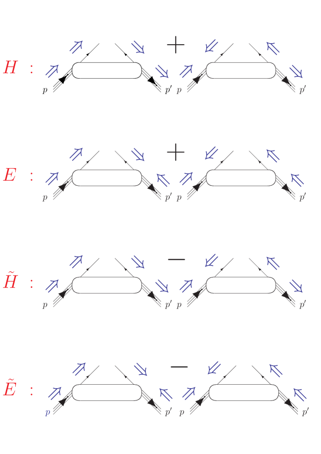
Figure 5: The four GPDs $H$, $E$, $\tilde{H}$ and $\tilde{E}$ correspond to the various quarks helicity and nucleon spin orientations.

Omitting the $Q^{2}$-dependence associated with QCD evolution equation, the GPDs depend on three independent variables: $x$, $\xi$ and $t$. $x$ varies between -1 and 1 and $\xi$ in principle also between -1 and 1 but, due to time reversal invariance, the range of $\xi$ is reduced between 0 and 1. If $|x|>\xi$, GPDs represent the probability amplitude of finding a quark (or an antiquark if $x<-\xi$) in the nucleon with a $+$ momentum fraction $x+\xi$ and of putting it back into the nucleon with a $+$ momentum fraction $x-\xi$ plus some transverse momentum “kick”, which is represented by $t$ (or $\Delta_{\perp}^{2}$).

The other region $-\xi<x<\xi$ implies that one “leg” in Fig. 3 (right panel) has a positive momentum fraction (a quark) while the other one has a negative one (an antiquark). In this region, the GPDs behave like a meson distribution amplitude and can be interpreted as the probability amplitude of finding a quark-antiquark pair in the nucleon. This kind of information on $q{\bar{q}}$ configurations in the nucleon and, more generally, the correlations between quarks (or antiquarks) of different momenta, are relatively unknown, and reveal the richness and novelty of the GPDs.

Each GPD is defined for a given quark flavor: $H^{q},E^{q},\tilde{H}^{q},\tilde{E}^{q}$ ($q=u,d,s,...$). $H$ and $\tilde{H}$ are a generalization of the PDFs of Eq. (1) measured in DIS. In the forward direction, one has the model independent relations :

$$H^{q}(x,0,0)\, = \left\{\begin{array}[]{cr}q(x),&\hskip 14.22636ptx\;>\;0\,,\\ -\bar{q}(-x),&\hskip 14.22636ptx\;<\;0\,.\end{array}\right.$$ (7)

$$\hskip 14.22636pt\tilde{H}^{q}(x,0,0)\, = \left\{\begin{array}[]{cr}\Delta q(x),&\hskip 14.22636ptx\;>\;0\,,\\ \Delta\bar{q}(-x),&\hskip 14.22636ptx\;<\;0\,.\end{array}\right.$$ (10)

The origin of these relations is the optical theorem and the symmetry of the forward Compton process, corresponding with zero four-momentum transfer, i.e. $\xi=0$ and $t=0$. Fig. 6 illustrates this relation.

Figure 6: The optical theorem : the cross section of the DIS process is equal to the imaginary part of the forward amplitude of the (doubly virtual) Compton process.

Also, at finite momentum transfer, there are model independent sum rules which relate the first moments of GPDs to the elastic FFs of Eq. (2):

$$\int_{-1}^{+1}dxH^{q}(x,\xi,t)\,=\,F_{1}^{q}(t)\;,\hskip 14.22636pt\int_{-1}^{+1}dxE^{q}(x,\xi,t)\,=\,F_{2}^{q}(t)\;,$$ (11)

$$\int_{-1}^{+1}dx\tilde{H}^{q}(x,\xi,t)\,=\,G_{A}^{q}(t)\;,\hskip 14.22636pt\int_{-1}^{+1}dx\tilde{E}^{q}(x,\xi,t)\,=\,G_{P}^{q}(t)\;.$$

Fig. 7 illustrates these sum rules.

Figure 7: Illustration of the sum rules of Eq. (11) linking the first $x$ moment of the GPDs to FFs. The integration on the $x$ momentum leads to a local operator (via the $\delta$ function in $y$).

One therefore sees that the PDFs and the FFs appear as simple limits or moments of the GPDs.

Similarly to the FFs, the $t$ variable in GPDs is the conjugate variable of the impact parameter (in the light-front frame) [1, 39, 40]. For $\xi=0$ (where $t=-\Delta_{\perp}^{2}$), one has threfore an impact parameter version of GPDs through a Fourier integral in tranverse momentum $\Delta_{\perp}$ :

$$H^{q}(x,{\bf b_{\perp}})=\int\frac{d^{2}{\bf\Delta_{\perp}}}{(2\pi)^{2}}e^{-i{\bf b_{\perp}\cdot\Delta_{\perp}}}H^{q}(x,0,-{\bf\Delta_{\perp}}^{2}).$$ (12)

At $\xi$=0, the GPD($x,0,t$) can then be interpreted as the probability of finding a parton with longitudinal momentum fraction $x$ at a given transverse distance (relative to the transverse c.m.) in the nucleon. In this way, the information contained in a traditional parton distribution, as measured in DIS, and the information contained within a form factor, as measured in elastic lepton-nucleon scattering, are combined and correlated in the GPD description.

The second moment of the GPDs is relevant to the nucleon spin structure. It was shown in Ref.[9] that there exists a (color) gauge-invariant decomposition of the nucleon spin: ${1\over 2}=J_{q}+J_{g}$, where $J_{q}$ and $J_{g}$ are respectively the total quark and gluon contributions to the nucleon total angular momentum. The second moment of the GPD’s gives (Ji’s sum rule) :

$$J_{q}\,=\,{1\over 2}\,\int_{-1}^{+1}dx\,x\,\left[H^{q}(x,\xi,t=0)+E^{q}(x,\xi,t=0)\right].$$ (13)

The total quark spin contribution $J_{q}$ decomposes (in a gauge invariant way) as $J_{q}={1\over 2}\Delta\Sigma+L_{q}$ where 1/2 $\Delta\Sigma$ and $L_{q}$ are respectively the quark spin and quark orbital contributions to the nucleon spin. $\Delta\Sigma$ can be measured through polarized DIS experiments, and its extracted value is shown in Table 2. One sees from Table 2 that the different determinations of $\Delta\Sigma$ all point to a value in the range 20 - 30 %.

On the other hand, for the gluons it is still an open question how to decompose the total angular momentum $J_{g}$ into orbital angular momentum, $L_{g}$, and gluon spin, $\Delta g$, parts, in such a way that both can be related to observables. For a discussion on recent developments in this active field, see [46] and references therein. At present, it is only known how to directly access the gluon spin contribution $\Delta g$ in experiment. It can be accessed in several ways: inclusive $c-\bar{c}$ or high $p_{T}$ hadron pairs production in polarized semi-inclusive DIS, semi-inclusive $\pi^{0}$, $\gamma$, jet,… production in polarized proton collisions and evolution of $g_{1}(x,Q^{2})$ through global fits of polarized data. At present $\Delta g$ can only be extracted with a large uncertainty, as can be seen from Table 2. While most determinations for $\Delta g$ indicate a too small value to fully explain the spin puzzle, it is clearly very worthwhile to reduce the uncertainty in its extraction by further measurements.

	DSSV08 [41]	BB10 [42]	LSS10 [43]	AAC08 [44]	NNRR12 [45]
$\Delta\Sigma(Q^{2})$	$0.25\pm 0.02$	$0.19\pm 0.08$	$0.21\pm 0.03$	$0.24\pm 0.07$	$0.31\pm 0.10$
$\Delta g(Q^{2})$	$-0.10\pm 0.16$	$0.46\pm 0.43$	$0.32\pm 0.19$	$0.63\pm 0.81$	$-0.2\pm 1.4$

Table 2: Comparison of different determinations of the first moments of the singlet and gluon polarised PDFs at the scale $Q^{2}=4$ GeV² in the $\overline{\mbox{MS}}$ scheme. All uncertainties shown are statistical only.

The sum rule of Eq. (13) in terms of the GPDs provides a model independent way of determining the quark orbital contribution to the nucleon spin and therefore completes the quark sector of the “spin-puzzle”.

Eq. (13) is actually a particular case of a more general rule on the $x$ moments of GPDs. The so-called polynomiality condition state that the $x^{n}$ moment of GPDs must be a polynomial in $\xi$ of order $n$ (for $n$ even, corresponding with non-singlet GPDs) or $n+1$ (for $n$ odd, corresponding with singlet GPDs), e.g. for the $H$ GPD :

$$if\,\,n\,\,even:\int_{-1}^{1}dx\,x^{n}H(x,\xi,t)=a_{0}+a_{2}\xi^{2}+a_{4}\xi^{4}+...+a_{n}\xi^{n},$$

$$if\,\,n\,\,odd:\int_{-1}^{1}dx\,x^{n}H(x,\xi,t)=a_{0}+a_{2}\xi^{2}+a_{4}\xi^{4}+...+a_{n+1}\xi^{n+1}.$$ (14)

There are similar rules for the GPDs $E$, $\tilde{H}$ and $\tilde{E}$. For the GPD $E$, the $a_{n+1}$ coefficient is the same as for $H$ except that it has the opposite sign. For the GPDs $\tilde{H}$ and $\tilde{E}$, the maximum $\xi$ power in Eq. (14) for singlet GPDs is $n-1$ (instead of $n+1$).

We note that in Eq. (14) only even powers of $\xi$ appear which is a consequence of the time reversal invariance which states that : $H(x,-\xi,t)=H(x,\xi,t)$.

Besides the polynomiality constraints on GPDs, the GPDs are also constrained by positivity conditions which should be taken into account both for nonzero and zero skewness parameter. The simplest of these conditions arises from requiring the positivity of the quark distribution in a transversely polarized nucleon. This imposes a relation between the $E$-type and $H$-type GPDs, for more details see Ref. [47].

As mentioned above, an ab initio calculation of soft matrix elements in general seems at present only pratical within lattice QCD. By its nature of discretizing the theory on an euclidean space-time lattice, lattice QCD can robustly calculate a few lowest moments of GPDs, which correspond to matrix elements of local operators. Although at present the calculations are being performed for unphysical pion masses, it is foreseeable that in the next few years calculations for such quantities at the physical point with controlled systematic uncertainties will become available. They can be used in the near future as additional constraints when confronting GPD parameterizations with experiment. We refer to the review paper of Ref. [48] for a recent review of lattice efforts in this field.

1.3 Generalized Transverse-Momentum dependent parton Distributions (GTMDs)

The GPDs can be considered as a particular limit of generalized parton correlation functions. The Generalized Parton Correlation Functions (GPCFs) provide a unified framework to describe the partonic information contained in a hadron. The GPCFs parameterize the fully unintegrated off-diagonal quark-quark correlator, depending on the full 4-momentum $k$ of the quark and on the 4-momentum $\Delta$ which is transferred by the probe to the hadron; for a classification see refs. [49, 50]. They have a direct connection with the Wigner distributions of the parton-hadron system [51, 52, 37], which represent the quantum mechanical analogues of the classical phase-space distributions.
When integrating the GPCFs over the light-cone energy component of the quark momentum one arrives at generalized transverse-momentum dependent parton distributions (GTMDs) which contain the most general one-body information of partons, corresponding to the full one-quark density matrix in momentum space. These GTMDs parameterize the following general unintegrated, off-diagonal quark-quark correlator for a hadron [50] :

$$W^{[\Gamma]}_{\Lambda^{\prime}\Lambda}(\Delta,\vec{k}_{\perp},x;\eta)=\frac{1}{2}\int\frac{{\mathrm{d}}y^{-}\,{\mathrm{d}}^{2}y_{\perp}}{(2\pi)^{3}} \,e^{i(xp^{+}y^{-}-\vec{k}_{\perp}\cdot\vec{y}_{\perp})}\,$$ (15)

$$\times\langle p^{\prime},\Lambda^{\prime}|\overline{\psi}(-\frac{y}{2})\Gamma\mathcal{W}\,\psi(\frac{y}{2})|p,\Lambda\rangle\big{|}_{y^{+}=0},$$

where the superscript $\Gamma$ stands for any element of the basis $\{1,\gamma_{5},\gamma^{\mu},\gamma^{\mu}\gamma_{5},i\sigma^{\mu\nu}\gamma_{5}\}$ in Dirac space, and $\Lambda$ ($\Lambda^{\prime}$) denote the helicities of initial (final) hadron respectively. A Wilson line $\mathcal{W}\equiv\mathcal{W}(-\frac{y}{2},\frac{y}{2}|n)$ ensures the color gauge invariance of the correlator, connecting the points $-\frac{y}{2}$ and $\frac{y}{2}$ via the intermediary points $-\frac{y}{2}+\infty\cdot n$ and $\frac{y}{2}+\infty\cdot n$ by straight lines. This induces a dependence of the Wilson line on the light-cone direction $n$. Furthermore, the parameter $\eta=\textrm{sign}(n^{0})$ gives the sign of the zeroth component of $n$, i.e. indicates whether the Wilson line is future-pointing ($\eta=+1$) or past-pointing ($\eta=-1$). Clearly, such correlators generalizes the GPD correlators introduced in Eq. (3) by allowing the quark operator to be also non-local in the transverse direction, i.e. besides the GPD arguments $x,\xi$, and $t$, the GTMDs also depend on the quark transverse momentum $\vec{k}_{\perp}$.

Figure 8: The GTMDs reduce to different parton distributions and form factors. By integrating over the quark transverse momentum $\vec{k}_{\perp}$, the GTMDs reduce to the GPDs, whereas the forward limit $\xi=0,t=0$ (i.e. $\Delta=0$) can in turn be parameterized in terms of TMDs, which are the quantities which enter semi-inclusive deep inelastic scattering processes. Integrating the TMDs over $\vec{k}_{\perp}$ gives rise to the forward parton distributions. The forward parton distributions are also obtained by taking the forward limit $\Delta=0$ in the GPDs. Integrating the GPDs over $x$ yields the form factors. In the middle row right column figure, “ff” stands for “fragmentation functions” which we do not discuss here.

At leading twist, there are sixteen complex GTMDs, which are defined in terms of the independent polarization states of quarks and hadron. In the forward limit $\Delta=0,$ they reduce to eight transverse-momentum dependent parton distributions (TMDs) which depend on the longitudinal momentum fraction $x$ and transverse momentum $\vec{k}_{\perp}$ of quarks, and therefore give access to the three-dimensional picture of the hadrons in momentum space. On the other hand, the integration over $\vec{k}_{\perp}$ of the GTMDs leads to eight GPDs which are probability amplitudes related to the off-diagonal matrix elements of the parton density matrix in the longitudinal momentum space. After a Fourier transform of $\vec{\Delta}_{\perp}$ to the impact-parameter space, they provide a three-dimensional picture of the hadron in a mixed momentum-coordinate space. The common limit of TMDs and GPDs is given by the standard parton distribution functions (PDFs), related to the diagonal matrix elements of the longitudinal-momentum density matrix for different polarization states of quarks and hadron. Fig. 8 illustrates how the GTMDs reduce to different parton distributions and form factors.

Although it has not been shown to date that the GTMDs can be accessed in a model independent way in experiment, they may however provide useful quantities to gain insight through model calculations of hadron structure, see e.g. [53].

2 From theory to data

Among the hard exclusive leptoproduction processes, the DVCS channel bears the best promises to extract the GPDs from experimental data using the leading-twist handbag diagram amplitude. Indeed, in DVCS, the hard perturbative part of the handbag involves only electromagnetic vertices (Fig. 3) while in Deeply Virtual Meson Electroproduction (DVMP), there are strong vertices involving a gluon exchange, see Fig. 9. In DVMP there is another soft non-perturbative quantity besides the GPDs that enters the calculation: the distribution amplitude (DA) of the meson which is produced. As the gluon virtuality needs to be hard to ensure the leading-twist amplitude, the endpoint behavior of the DA can potentially lead to strong power corrections to the leading-twist amplitude. In this review, we focus on the DVCS process on the proton.

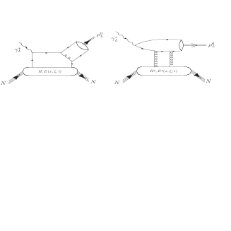
Figure 9: The leading-twist handbag diagram for DVMP involving quark (left) and gluon (right) GPDs. We note that the factorization between a hard scattering process and GPDs and DAs for DVMP has been demonstrated only for longitudinally polarized incoming photons.

2.1 Compton Form Factors

Four independent variables are needed to describe the 3-body final state reaction $e(p_{e})p(p_{p})\to e^{\prime}(p_{e}^{\prime})p(p_{p}^{\prime})\gamma(p_{\gamma})$ at a fixed beam energy $E_{e}$. They are usually chosen as $Q^{2}$, $x_{B}$, $t$ and $\phi$ where $Q^{2}=-(p_{e}-p_{e}^{\prime})^{2}$, $x_{B}=\frac{Q^{2}}{2p_{p}\cdot q}$ (with $q$ the virtual photon four-momentum), $t=(p_{p}-p_{p}^{\prime})^{2}$ and $\phi$ is the azimuthal angle between the electron scattering plane and the hadronic production plane (see Ref. [54] for its explicit definition within the Trento convention). See Fig. 10 for an illustration of these kinematical quantities.

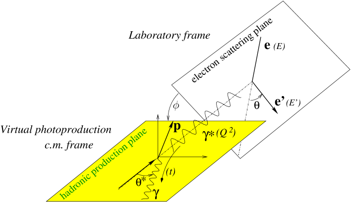
Figure 10: Reference frames and relevant variables for the description of the $ep\rightarrow e^{\prime}p^{\prime}\gamma$ reaction.

At leading-twist, the GPDs depend on the three variables : $x$, $\xi$ and $t$ where the variable $\xi$ is related to $x_{B}$ by: $\xi=x_{B}/(2-x_{B})$. In principle, GPDs depend on $Q^{2}$ as well. However, this dependence can be predicted and calculated through the evolution equations and does not reflect the non-perturbative structure of the nucleon. For simplicity, we will not write the dependence on $Q^{2}$ explicitly in the following. The variables $\xi$ and $t$ can be accessed by measuring the kinematics of the scattered electron and of the final state photon and/or proton. However, the variable $x$ is not experimentally accessible. In the calculation of the DVCS amplitude of the handbag diagram of Fig. 3, the variable $x$ is integrated over. The DVCS amplitude is written as:

$$M_{DVCS}=\epsilon_{\mu}(q)\epsilon^{*}_{\nu}(p_{\gamma})H^{\mu\nu}_{L.O.\,DVCS}$$ (16)

where $\epsilon_{\mu}(q)$ and $\epsilon^{*}_{\nu}(p_{\gamma})$ are respectively the polarisation 4-vectors of the (virtual) initial and final photons and:

$$H^{\mu\nu}_{L.O.\,DVCS}$$ (17)

$$= {1\over 2}\,\left[\tilde{p}^{\mu}n^{\nu}+\tilde{p}^{\nu}n^{\mu}-g^{\mu\nu}\right]\;\int_{-1}^{+1}dx\left[{1\over{x-\xi+i\epsilon}}+{1\over{x+\xi-i\epsilon}}\right]$$

$$\times \left[H^{p}_{DVCS}(x,\xi,t)\;\bar{N}(p^{{}^{\prime}})\gamma.nN(p)+\;E^{p}_{DVCS}(x,\xi,t)\;\bar{N}(p^{{}^{\prime}})i\sigma^{\kappa\lambda}{{n_{\kappa}\Delta_{\lambda}}\over{2m}}N(p)\right]$$

$$+ \;{1\over 2}\,\left[-i\varepsilon^{\mu\nu\kappa\lambda}\tilde{p}_{\kappa}n_{\lambda}\right]\;\int_{-1}^{+1}dx\left[{1\over{x-\xi+i\epsilon}}-{1\over{x+\xi-i\epsilon}}\right]$$

$$\times \left[\tilde{H}^{p}_{DVCS}(x,\xi,t)\bar{N}(p^{{}^{\prime}})\gamma.n\gamma_{5}N(p)+\tilde{E}^{p}_{DVCS}(x,\xi,t)\bar{N}(p^{{}^{\prime}})\gamma_{5}{{\Delta\cdot n}\over{2m}}N(p)\right]\;,$$

with $\varepsilon_{0123}=+1$ and the lightlike vectors along the positive and negative $z$-directions: $\tilde{p}^{\mu}=P^{+}/\sqrt{2}(1,0,0,1)$ and $n^{\mu}=1/P^{+}\cdot 1/\sqrt{2}(1,0,0,-1)$.

One readily sees from Eq. (17) that the variable $x$ which is a “mute” variable is integrated over. It is also weighted by the $\frac{1}{x\pm\xi\mp i\epsilon}$ factors, which originate from the propagator of the quark in the handbag diagram of Fig. 3 (left panel).

The DVCS amplitude contains convolution integrals of the form :

$$\int_{-1}^{+1}dx{{H(x,\xi,t)}\over{x-\xi+i\epsilon}}={\cal P}\int_{-1}^{+1}dx{H(x,\xi,t)\over{x-\xi}}-i\pi H(\xi,\xi,t),$$ (18)

and analogously for the GPDs $E$, $\tilde{H}$ or $\tilde{E}$. In Eq. (18), we have decomposed the expression into a real and an imaginary part where ${\cal P}$ denotes the principal value integral. This means that the maximum information that can be extracted from the experimental data in the DVCS process at a given ($\xi,t$) point is $GPD(\pm\xi,\xi,t)$ or/and $\int_{-1}^{+1}dx{H(\mp x,\xi,t)\over{x\pm\xi}}$. The former is accessed when an observable sensitive to the imaginary part of the DVCS amplitude is measured, such as single beam- or target-spin observables, while the latter is accessed when an observable sensitive to the real part of the DVCS amplitude is measured, such as double beam- or target-spin observables or beam charge sensitive observables. The unpolarized cross section is sensitive to both the real and imaginary parts of the DVCS amplitude.

There are therefore in principle eight GPD-related quantities that can be extracted from the DVCS process:

$$H_{Re}(\xi,t) \equiv {\cal P}\int_{0}^{1}dx\left[H(x,\xi,t)-H(-x,\xi,t)\right]C^{+}(x,\xi),$$ (19)

$$E_{Re}(\xi,t) \equiv {\cal P}\int_{0}^{1}dx\left[E(x,\xi,t)-E(-x,\xi,t)\right]C^{+}(x,\xi),$$ (20)

$$\tilde{H}_{Re}(\xi,t) \equiv {\cal P}\int_{0}^{1}dx\left[\tilde{H}(x,\xi,t)+\tilde{H}(-x,\xi,t)\right]C^{-}(x,\xi),$$ (21)

$$\tilde{E}_{Re}(\xi,t) \equiv {\cal P}\int_{0}^{1}dx\left[\tilde{E}(x,\xi,t)+\tilde{E}(-x,\xi,t)\right]C^{-}(x,\xi),$$ (22)

$$H_{Im}(\xi,t) \equiv H(\xi,\xi,t)-H(-\xi,\xi,t),$$ (23)

$$E_{Im}(\xi,t) \equiv E(\xi,\xi,t)-E(-\xi,\xi,t),$$ (24)

$$\tilde{H}_{Im}(\xi,t) \equiv \tilde{H}(\xi,\xi,t)+\tilde{H}(-\xi,\xi,t),$$ (25)

$$\tilde{E}_{Im}(\xi,t) \equiv \tilde{E}(\xi,\xi,t)+\tilde{E}(-\xi,\xi,t),$$ (26)

with the coefficient functions $C^{\pm}$ defined as :

$$C^{\pm}(x,\xi)=\frac{1}{x-\xi}\pm\frac{1}{x+\xi}$$ (27)

and where one has reduced the $x$-range of integration from $\{-1,1\}$ to $\{0,1\}$ in the convolutions.

The functions $H_{Re},H_{Im}$, etc. on the lhs of Eqs. (19 - 26), which depend on the two kinematical variables $\xi$ and $t$, accessible in experiment, are called the Compton Form Factors (CFFs)  .

For further use, we also introduce the complex functions as :

$${\cal H}(\xi,t)\equiv H_{Re}(\xi,t)-i\pi H_{Im}(\xi,t),$$ (28)

and analogously for the other GPDs.

In the following, we will also use the notation:

$$H_{+}(x,\xi,t) \equiv H(x,\xi,t)-H(-x,\xi,t),$$

$$E_{+}(x,\xi,t) \equiv E(x,\xi,t)-E(-x,\xi,t),$$ (29)

$$\tilde{H}_{+}(x,\xi,t) \equiv \tilde{H}(x,\xi,t)+\tilde{H}(-x,\xi,t),$$

$$\tilde{E}_{+}(x,\xi,t) \equiv \tilde{E}(x,\xi,t)+\tilde{E}(-x,\xi,t),$$ (30)

since these are the so-called singlet ($\mathcal{C}$ = +1) GPD combinations, which enter in the CFFs, and consequently in the DVCS observables.

2.2 The Bethe-Heitler process

The DVCS process is not the only amplitude contributing to the $ep\to ep\gamma$ reaction. There is also the Bethe-Heitler (BH) process, in which the final state photon is radiated by the incoming or scattered electron and not by the nucleon itself. This is illustrated in Fig. 12. The BH process leads to the same final state as the DVCS process and interferes with it. Since the nucleon form factors $F_{1}$ and $F_{2}$ can be considered as well-known at small $t$, the BH process is precisely calculable theoretically. The BH cross section has the very distinct feature to sharply rise around $\phi$=0^∘ and 180^∘. These are the regions where the radiated photon is emitted in the direction of the incoming electron or the scattered one. The strong enhancements when the outgoing photon is emitted in the electron-proton plane is due to singularities (for massless electrons) in the electron propagators.

In those regions, a small variation in the kinematical variables $Q^{2}$, $x_{B}$, $t$ or $\phi$ produces strong variations in the cross section. For instance, Fig. 11 shows that a variation of $x_{B}$ by 1% around the particular kinematical setting $x_{B}$=0.300, $Q^{2}$=2.500 GeV², $t$=-0.200 GeV², $E_{e}$=5.750 GeV induces a variation of almost 10% at very low and large $\phi$. It should be noted that, even at $\phi$=180^∘, this relative difference remains more than 5%. Experiments should therefore as much as possible quote and control the values of the kinematic variables at least at the percent level to achieve a few percent accuracy on the BH+DVCS cross sections.

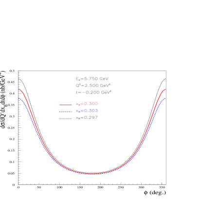
Figure 11: The theoretical cross section of the BH process at the central kinematics $E_{e}$=5.750 GeV, $x_{B}$=0.300, $Q^{2}$=2.500 GeV², $t$=-0.200 GeV², with variations of 1% in $x_{B}$.

The importance of the BH relative to the DVCS strongly depends on the ($x_{B}$, $Q^{2}$, $t$, $\phi$) phase space regions. It can largely dominate or be negligible compared to DVCS. The presence of BH can actually be considered as an asset when one measures observables which are sensitive to the BH-DVCS interference. The BH can then act as an amplifier for the DVCS process and gives access to CFFs in a linear fashion, instead of a bilinear one if only DVCS was present.

Figure 12: The cross section of the $ep\to ep\gamma$ reaction is proportional to the squared amplitude : $\mid M_{DVCS}+M_{BH}\mid^{2}$. The DVCS process is proportional to GPDs while the BH process is proportional to FFs. The two processes interfere.

2.3 Experimental observables

As illustrated in Fig. 5, the four GPDs reflect the four independent spin/helicity nucleon/quark combinations in the handbag diagram. Therefore, the way to separate them is to use the spin degrees of freedom of the beam and of the target and measure various polarization observables. In Ref. [55], analytical relations linking the observables and the CFFs have been derived for the $ep\to ep\gamma$ reaction, considered as the (coherent) sum of the BH and DVCS processes. We present here a few of them:

$$\Delta\sigma_{LU}\propto\sin\phi\;\;Im\{F_{1}\mathcal{H}+\xi(F_{1}+F_{2})\tilde{\mathcal{H}}-kF_{2}\mathcal{E}+...\}$$ (31)

$$\Delta\sigma_{UL}\propto\sin\phi\;\;Im\left\{F_{1}\tilde{\mathcal{H}}+\xi(F_{1}+F_{2})\left(\tilde{\mathcal{H}}+\frac{x_{B}}{2}\mathcal{E}\right)-\xi kF_{2}\tilde{\mathcal{E}}+...\right\}$$ (32)

$$\Delta\sigma_{LL}\propto(A+B\cos\phi)\;\;Re\left\{F_{1}\tilde{\mathcal{H}}+\xi(F_{1}+F_{2})\left(\mathcal{H}+\frac{x_{B}}{2}\mathcal{E}\right)+...\right\}$$ (33)

$$\Delta\sigma_{Ux}\propto\sin\phi\;\;Im\{k(F_{2}\mathcal{H}-F_{1}\mathcal{E})+...\}$$ (34)

where $\Delta\sigma$ stands for a difference of polarized cross sections, with the first index referring to the polarization of the beam (“U” for unpolarized and “L” for longitudinally polarized) and the second one to the polarization of the target: “U” for unpolarized, ‘L” for longitudinally polarized and “x” or “y” for a transversely polarized target. Indeed, in this latter case, there are two independent polarization directions: “x” is in the hadronic plane and “y” is perpendicular to it (see Fig. 10). Furthermore, the kinematical variable $k$ is defined as : $k=-t/(4m_{N}^{2})$.

The difference of polarized cross sections in Eqs. (31-34) are sensitive only to the BH-DVCS interference term. The CFFs arise from the DVCS process while the $F_{1}$ and $F_{2}$ FFs originate from the BH process and only products of FFs and CFFs appear, thus providing access to CFFs in a linear fashion. At leading order in a $\frac{1}{Q}$ expansion, only $\sin\phi$ or $\cos\phi$ modulations appear. One also notices in general that single spin observables are sensitive to the imaginary CFFs while double-spin observables are sensitive to the real CFFs.

In a first approximation, neglecting terms multiplied by kinematical factors such as $\xi$, $x_{B}$ and $k$, one can see that, on a proton target, $\Delta\sigma_{LU}$ is dominantly sensitive to $H_{Im}^{p}$, $\Delta\sigma_{UL}$ to $\tilde{H}_{Im}^{p}$, $\Delta\sigma_{LL}$ to $\tilde{H}_{Re}^{p}$ and $\Delta\sigma_{UT}$ to $H_{Im}^{p}$ and $E_{Im}^{p}$. For a neutron target, the sensitivity of these spin observables to the CFFs changes as the values of the FFs are different (in particular, $F_{1}\approx 0$ at small $t$). Thus, on a neutron target, $\Delta\sigma_{LU}$ is dominantly sensitive to $E_{Im}^{n}$ and $\tilde{H}_{Im}^{n}$, $\Delta\sigma_{UL}$ to $\tilde{H}_{Im}^{n}$, $\Delta\sigma_{LL}$ to $H_{Re}^{n}$ and $\Delta\sigma_{UT}$ to $H_{Im}^{n}$.

Here, we have displayed explicitely the “$p$” and “$n$” superscripts to underline that GPDs on the proton and on the neutron are not equal. The relations expressing the “$p$” and “$n$” GPDs entering the DVCS amplitudes, in terms of the $u$- and $d$-quark contributions, are given for the GPD $H$ by :

$$H^{p}(\xi,\xi,t)=\frac{4}{9}H^{u}(\xi,\xi,t)+\frac{1}{9}H^{d}(\xi,\xi,t),$$ (35)

$$H^{n}(\xi,\xi,t)=\frac{4}{9}H^{d}(\xi,\xi,t)+\frac{1}{9}H^{u}(\xi,\xi,t),$$ (36)

and similarly for the GPDs $E$, $\tilde{H}$ or $\tilde{E}$.

In summary, given the number of variables on which the GPDs depend (three, omitting the $Q^{2}$-dependence), the convolution over $x$ in the amplitudes, the presence of the BH process with it singularities, the number of CFFs (eight at leading twist), the quark flavor decomposition, not to mention the $Q^{2}$ evolution and higher-twist corrections, it is clearly a non-trivial task to extract the GPDs from the experimental data and, ultimately to map them in the three variables $x,\xi,t$. It requires a broad experimental program measuring several DVCS (or DVMP) spin observables on proton and neutron targets over large ranges in $x_{B}$ and $t$ (and $Q^{2}$).

There are several strategies to make progress in such a program. One of them is, as an intermediate step, to extract the CFFs from DVCS data for a given $(\xi,t)$ point by fitting the $\phi$ distribution at a given beam energy. This can be done in an essentially model-independent way provided one has enough constraints, i.e. experimental observables, to extract the eight CFFs. As we will see in section 4, even if there are only two observables which are measured, to be fitted by eight CFFs taken as free parameters, making the problem a priori largely under-constrained, some results can still be obtained due to the domaince of such few observables by one or two CFFs. However, this is only the first step of the program, since the $x$ dependence still needs to be uncovered, in principle with the help of a model with adjustable parameters. The problem can be simplified with the help of dispersion relations which we will discuss in section 3.4. They can in principle reduce from eight to five the number of GPD quantities to be extracted. They state, in a model-independent way, that the real part CFFs defined by Eqs. (19 - 22) are actually integrals over $\xi$ of their respective imaginary part CFFs defined by Eqs. (23 - 26). In this approach, there is in addition a real subtraction constant (at fixed $\xi$ and $t$) which intervenes and makes the number of independent quantities to be five in total. To apply dispersion relations, it is needed to measure data over a very wide range in $\xi$ (at fixed $t$) unless one has good reasons to truncate the integral or to extrapolate. Another strategy consists in fitting directly the experimental observables by a model which has for each GPD $H$, $E$, $\tilde{H}$ or $\tilde{E}$, a parameterization of the full $x,\xi,t$-dependence with parameters to be fitted. We will discuss these various approaches below.

Let us also mention that there is an experimental way to measure indepedently the $x$ and $\xi$-dependence of GPDs. The double-DVCS process consists of the DVCS process with a virtual (space-like or time-like) photon in the final state. In the case of a final timelike photon, the virtuality of this second photon can be measured and varied, thus providing an extra lever arm and allowing to measure the GPDs for each $x,\xi,t$ values independently (though with some limitations if the final photon is timelike) [56, 57]. However, since the cross section of such process is reduced by a factor $\alpha\approx 1/137$, and since one needs to make measurements above the vector meson resonance region to avoid the strong vector meson processes, the double DVCS has not revealed so far to be a practical way to access GPDs.

We now review the existing DVCS measurements, limiting ourselves to the large and intermediate $x_{B}$ regions.

2.4 Existing DVCS measurements

Three experiments have provided these past 10 years DVCS data which can potentially lend themselves to a GPD interpretation. These are the Hall A and CLAS experiments from JLab (with a $\approx$ 6 GeV electron beam energy) and the HERMES experiment at DESY (with a $\approx$ 27 GeV electron or positron beam energy).

2.4.1 JLab Hall A

The $ep\to e^{\prime}p^{\prime}\gamma$ reaction was measured in the JLab Hall A experiment [58] by detecting only the scattered electron in a high resolution ($\frac{\delta p}{p}\approx 10^{-4}$ for momentum) arm spectrometer and the real photon in an electromagnetic calorimeter ($\frac{\sigma E}{\sqrt{E}}\approx 4$ % for energy). A cut on the missing mass of the proton which clearly stood out over a small background was used to unambiguously identify the exclusive process.

The Hall A experiment measured the 4-fold beam-polarized and unpolarized differential cross sections $d\sigma/dx_{B}dQ^{2}dtd\phi$, i.e. without any integration over an independent variable, as a function of $\phi$, for four $-t$ values (0.17, 0.23, 0.28 and 0.33) at the average kinematics: $<x_{B}>=0.36$ and $<Q^{2}>=2.3$ GeV². The beam-polarized cross sections have also been measured at $<Q^{2}>=1.5$ GeV² and $<Q^{2}>=1.9$ GeV². Fig. 13 shows these results. The particular shape in $\phi$ of the BH contribution in the unpolarized cross section (red curve in the upper panels of Fig. 13) is easily recognizable. The difference between the red curve and the data is the contribution of the DVCS process and therefore of the GPDs.

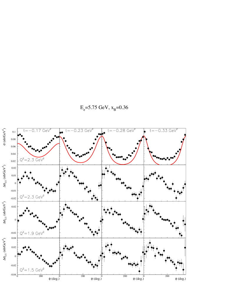
Figure 13: The panels of the top row show the DVCS/BH unpolarized cross sections on the proton, as a function of the $\phi$ angle, measured by the JLab Hall A collaboration [58]. The average kinematics is $<x_{B}>$=0.36, $<Q^{2}>$=2.3 GeV² and $<-t>$=0.33, 0.28, 0.23 and 0.17 GeV² (left to right). The red curves show the BH contribution. The bottom panels show the difference of beam-polarized cross section as a function of $\phi$ for the same kinematics at $<Q^{2}>$=2.3 GeV² (second row), $<Q^{2}>$=1.9 GeV² (third row) and $<Q^{2}>$=1.5 GeV² (fourth row).

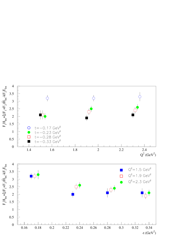
Figure 14: Top panel: $Q^{2}$-dependence of the combination of CFFs: $F_{1}H_{Im}+\xi(F_{1}+F_{2})\tilde{H}_{Im}-kF_{2}E_{Im}$ for four different values of $-t$, as extracted from the fit of the beam-polarized cross sections of Fig. 13 (three bottom panels). Bottom panel: $t$-dependence of the same combination of CFFs as extracted from the fit of the beam-polarized cross sections of Fig. 13 (three bottom panels).

The difference of beam-polarized cross sections, i.e. $\Delta\sigma_{LU}$, is displayed in the three lower panels of Fig. 13. In the leading order $\frac{1}{Q}$ expansion, the amplitude of the sinusoidal is directly proportional to the combination of CFFs: $F_{1}\mathcal{H}+\xi(F_{1}+F_{2})\tilde{\mathcal{H}}-kF_{2}\mathcal{E}$ (see Eq. (31)). Fitting these sinusoids has thus permitted to extract the $Q^{2}$-dependence of this combination of CFFs at four different $t$ values. The results of these fits is presented in Fig. 14. At leading-twist, GPDs and CFFs are predicted to be $Q^{2}$ independent and the data seem to exhibit this scaling feature. Although the $Q^{2}$ lever arm is very limited ($\approx$ 1 GeV²), this is a very encouraging sign that one can access the leading twist handbag process at the JLab kinematics.

We also mention that the beam spin asymmetry of the DVCS+BH process on the neutron $en\to en\gamma$ has been measured in an exploratory way by the JLab Hall A collaboration at one single $(<x_{B}>,<Q^{2}>)$ value (0.36,1.9) as a function of $t$ [59]. Although these results are encouraging and might possibly give some first constraints on the $E_{Im}$ CFF, we decide, in this review, to focus on the proton channel. There is a variety of observables which have been measured over a wide phase space for this latter process. This should give the strongest constraints on the GPD models and fits.

2.4.2 JLab Hall B

The JLab CLAS collaboration uses a large acceptance spectrometer and has measured the DVCS process by detecting the three particles of the final state, i.e. the scattered electron, the recoil proton and the produced real photon, over a much broader phase space than in Hall A. Since CLAS has a lesser resolution ($\frac{\delta p}{p}\approx 10^{-2}$ for momentum) than the Hall A arm spectrometers, the kinematic redundancy and overconstraint due to the detection of the full final state is the best way to ensure the exclusivity of the process.

Beam-polarized and unpolarized cross-sections measurements are under way  [60] but to this day, only beam spin asymmetries, i.e. the ratio of $\Delta\sigma_{LU}$ to the unpolarized cross section, and longitudinally polarized target asymmeties, i.e. the ratio of $\Delta\sigma_{UL}$ to the unpolarized cross section, have been measured. These asymmetries are observables which are relatively straightforward to extract experimentally since, in a first order approximation, normalization factors such as the efficiency/acceptance of the detector and, more generally, many sources of systematic errors cancel in the ratio. Both asymmetries have a shape close to a sin$\phi$ like Eq. (31) and (32) were predicting. The beam spin asymmetry was fitted by a function of the form $a\sin\phi/(1+c\cos\phi+d\cos 2\phi)$. Fig. 15 (left panel) shows the value of this fitted asymmetry at $\phi$ = 90^∘ for the $\approx$60 ($x_{B},Q^{2},t$) bins covered by CLAS and which were measured with a 5.77 GeV beam.

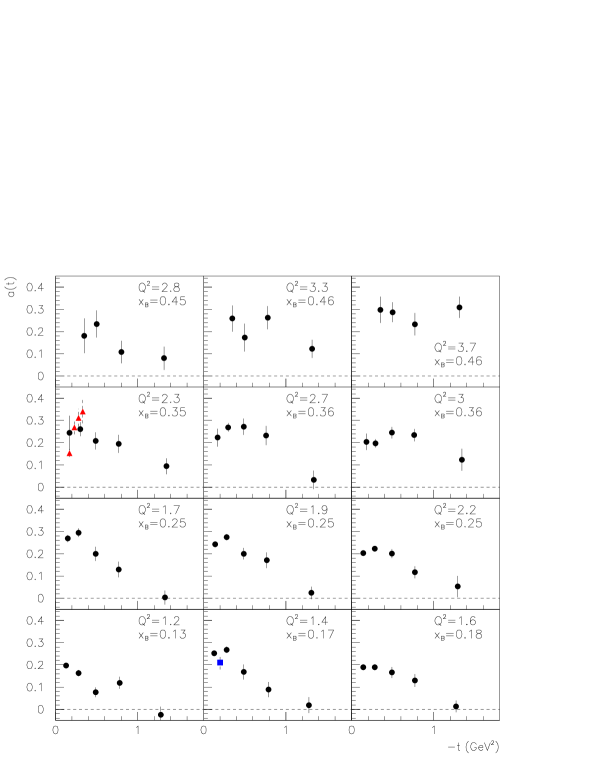
Figure 15: DVCS-BH beam spin asymmetry at $\phi$ = 90^∘ as a function of $t$ for different ($x_{B}$,$Q^{2}$) bins, as measured by the JLab Hall B/CLAS collaboration [61] (black solid circles). The red empty triangles are the beam spin asymmetries derived from the ratio of the beam-polarized and unpolarized cross sections of Hall A (see Fig. 13). The blue square point is the pionner measurement from the CLAS collaboration [62].

Figure 16: The $\sin(\phi)$ moments of the azimuthal moment of the DVCS-BH longitudinally polarized target asymmetry [63]. Left: Three bins $-t$, integrated over $x_{B}$; Right: Three bins in $x_{B}$, integrated over $t$.

Figure 17: Selection of ten DVCS-BH asymmetry $\phi$-moments as a function of $t$ as measured by HERMES. All moments in this figure are expected to be non-null in the leading $\frac{1}{Q}$ expansion but for the $A_{UL}^{\sin 2\phi}$ moment (bottom right plot).

The longitudinally polarized target asymmetries are displayed in Fig. 16. These observables show a $\sin\phi$-like shape, as predicted by theory (see Eq. (32)), and their $\sin\phi$ moment $A_{UL}^{\sin\phi}$ is presented in the figure. Here we extend the subscript notation of Eqs. (31) to (34) to asymmetry moments $A$, where the upperscript denotes the particular azumuthal moment considered. The use of a polarized target limited the statistics and the moments could be extracted only for 3 ($x_{B},Q^{2},t$) bins.

2.4.3 HERMES

At higher energies, $x_{B}\approx$ 0.1, the HERMES collaboration has carried out a measurement of ALL independent DVCS observables, except for cross sections: beam spin asymmetries [64, 65], longitudinally polarized target asymmetries [66], transversally polarized target asymmetries [67, 68], beam charge asymmetries [69, 70, 71] and all associated beam spin/target spin and spin/beam-charge double asymmetries. In a first stage, the HERMES experiment requested the detection of the scattered electron (or positron) and of the final real photon. Then, a cut on the missing mass of the proton was applied. The width of this missing mass peak being more than 1 GeV, a substantial background subtraction had to be performed. In a second stage, the HERMES spectrometer was completed by a recoil detector allowing the detection of the recoil proton and therefore a complete identification of the DVCS final state. The kinematics being then overconstrained, this allowed for a much cleaner selection of the exclusive reaction with a reduction of the contamination of non-DVCS events at the level of less than 1% [72]. In this “pure” DVCS samples, the amplitudes of beam-spin asymmetries were actually found to be somewhat larger (by about 10% in average).

HERMES used a positron beam as well as an electron beam and the target spin asymmetries have a different sensitivity to the BH+DVCS amplitude according to the charge of the beam. To describe such correlated charge and beam-spin asymmetries, one therefore introduces a second index (“I” or “DVCS”) for the labelling of the asymmetries, according to (for instance for the beam-spin asymmetries):

$$A_{\{LU,DVCS\}}=\frac{(\sigma^{+}_{+}(\phi)-\sigma^{+}_{-}(\phi))+(\sigma^{-}_{+}(\phi)-\sigma^{-}_{-}(\phi))}{\sigma^{+}_{+}(\phi)+\sigma^{+}_{-}(\phi)+\sigma^{-}_{+}(\phi)+\sigma^{-}_{-}(\phi)},$$ (37)

$$A_{\{LU,I\}}=\frac{(\sigma^{+}_{+}(\phi)-\sigma^{+}_{-}(\phi))-(\sigma^{-}_{+}(\phi)-\sigma^{-}_{-}(\phi))}{\sigma^{+}_{+}(\phi)+\sigma^{+}_{-}(\phi)+\sigma^{-}_{+}(\phi)+\sigma^{-}_{-}(\phi)},$$ (38)

where the superscript represents the charge of the beam and the subscript the beam (or target) spin projection. At leading-twist, only the asymmetries with an “I” subscript can be sensitive to GPDs while the ones with the “DVCS” subscript are null.

All DVCS azimuthal asymmetries have at leading twist a general sine, cosine or constant shape (see Eqs. 31-34 for a few examples), slightly modulated by the $\phi$-dependence of the denominator. The sine, cosine and constant moments of the nine asymmetries which are expected to be non-null in the leading-twist handbag formalism are displayed in Fig. 17. We added as a tenth observable the $A_{UL}^{\sin 2\phi}$ moment (bottom right plot) which is expected to be power suppressed in this approximation. However the data show a 2- to 3-standard deviation difference from zero. If one doesn’t consider this difference as a statistical fluctuation, it is a puzzle as it cannot be described by any leading-twist handbag calculation. Indeed, HERMES extracted also the “DVCS-subscript” asymmetries (see Eq. 38), as well as several $\sin 2\phi$, $\cos 2\phi$ or $\cos 3\phi$ moments, which are expected to be null in the hypothesis of DVCS leading-twist dominance. We do not display here these data but they were all found to be compatible with zero within error bars. Except for this puzzling $A_{UL}^{\sin 2\phi}$ moment, this gives further support to the idea that higher-twist contributions are small at the currently finite $Q^{2}$ values explored, confirming the first conclusions drawn from the JLab Hall A data.

In Fig. 17, we display only the $t$-dependence of these moments at the average $x_{B}$ and $Q^{2}$ values of 0.09 and 2.5 GeV² respectively. The data were taken with a 27.6 GeV beam energy. HERMES also measured the $x_{B}$- and $Q^{2}$-dependences, with the other kinematic variables fixed. Also, in this figure, the data correspond to data analysis carried out without the recoil detector.

We also mention that the HERMES collaboration has measured the DVCS+BH charge, beam spin and longitudinally polarized target asymmetries with a deuterium target [73, 74]. Such process is dominated by the incoherent DVCS+BH process on the proton and the results are in general consistent (with larger uncertainties) with the proton data shown in Fig. 17.

We finish this section by mentioning that the unpolarized $ep\to ep\gamma$ cross section has also been measured at much higher energy (30 $<W<$ 120 GeV, 2 $<Q^{2}<$ GeV² where $W$ is the center of mass energy of the $\gamma^{*}-p$ system), by the H1 and ZEUS collaborations [75, 76]. At such large $W$ (i.e. low $x_{B}$), the DVCS process is sensitive mostly to “gluon” GPDs which we do not cover in this review.

3 Models of GPDs and dispersive framework for DVCS

In this section, we review a few current state-of-the-art parameterizations of GPDs. We distinguish three families of models: models based on double distributions (VGG and GK), the dual parameterization and the Mellin-Barnes model.

3.1 Double distributions / Regge phenomenology: the VGG and the GK models

3.1.1 ($x$,$\xi$) dependence and Double Distributions

Double Distributions (DDs) were originally introduced by A. Radyushkin [77, 78] and D. Muller et al. [8]. They provide an elegant guideline to parameterize the ($x$,$\xi$) dependence of the GPDs which automatically satisfies the polynomiality relations (see Eq. (14)).

The idea of the DDs is to decorrelate the transferred longitudinal momentum ($\Delta$) from the initial nucleon momentum $P$ (see Fig. 3-right). In the light cone frame, one introduces then the new variables $\alpha$ and $\beta$ such that the initial quark has a longitudinal momentum $\beta P^{+}-\frac{1}{2}(1+\alpha)\Delta^{+}$ (see Fig. 18-left), instead of $(x+\xi)P^{+}$ (see Fig. 3-left). Since, by definition, $-2\xi=\frac{\Delta^{+}}{P^{+}}$, this means that $x=\beta+\alpha\xi$. The variable $\alpha$ is playing the role of $\xi$, the fraction of longitudinal momentum of the transfer, but the difference is that $\alpha$ is now an absolute value, i.e. it has no reference to the (average) initial nucleon momentum, unlike $\xi$. The link between a GPD and a DD is then only a change of variables, i.e. from $(\alpha,\beta)$ to $(x,\xi)$, such that :

$$GPD^{q}(x,\xi)=\int_{-1}^{1}d\beta\int_{-1+\mid\beta\mid}^{1-\mid\beta\mid}d\alpha\delta(x-\beta-\xi\alpha)DD(\alpha,\beta)$$ (39)

Figure 18: Left: illustration of the $\langle p^{\prime}|\bar{\psi}_{q}(0)\mathcal{O}\psi_{q}(y)|p\rangle$ matrix element in terms of the $\alpha$ and $\beta$ variables, instead of $x$ and $\xi$ (see Fig. 3-right). Right: the integration over the $(\alpha,\beta)$ variables, in order to relate DDs and GPDs, takes place over the $\beta=x-\xi\alpha$ straight line ”inside” the rhombus defined by the equation $\mid~{}\beta~{}\mid~{}+~{}\mid~{}\alpha~{}\mid~{}\leq~{}1$. The slope of the straight line is given by $\xi$ and its intercept at $\alpha=0$ is given by $x$.

One should integrate on all values/combinations of $\alpha$ and $\beta$ which produce the $(x,\xi)$ variables. Given that $x=\beta+\xi\alpha$, one has actually only a one-dimensionnal integral. The limits of the integration on the $\alpha$ and $\beta$ variables are constrained by the fact that $x$ has to be comprised between -1 and 1 and $\xi$ between 0 and 1, so that one has always $\mid x\mid+\mid\alpha\mid\leq 1$. This constraint means that the integration over the variables $\alpha$ and $\beta$ takes place over the $\beta=x-\xi\alpha$ straight line “inside” the rhombus defined by the equation $\mid\beta\mid+\mid\alpha\mid\leq 1$ (see Fig. 18-right).

Due to the linear relation between $x$ and $\xi$ imposed by the $\delta$ function, the polynomiality relation is automatically satisfied: the $x^{n}$ moment of Eq. (39) will always produce a $\xi^{n}$ power.

An advantage of the DDs is that the ($\alpha$,$\beta$) dependence can be more conveniently infered than the ($x$,$\xi$)-dependence. The matrix element corresponding to Fig. 18-left can be written:

$$\langle p+\Delta|\bar{\psi}_{q}(0)\mathcal{O}\psi_{q}(y)|p\rangle$$ (40)

where we can consider two “extreme” cases. When there is no longitudinal momentum transfer brought by the photon, i.e. $\Delta=0$, one gets :

$$\langle p|\bar{\psi}_{q}(0)\mathcal{O}\psi_{q}(y)|p\rangle{\Bigg{|}}_{y^{+}=\vec{y}_{\perp}=0}$$ (41)

and one recovers, as it should, the forward matrix element of Eq. (1) and which is equal to the standard inclusive PDF, the forward limit of GPDs.

However, there is now a second, new, limiting case : when $P=0$ and $\Delta\neq 0$, which is a case that couldn’t be considered before, since $\Delta$ was proportional to $P$ :

$$\langle\Delta|\bar{\psi}_{q}(0)\mathcal{O}\psi_{q}(y)|0\rangle{\Bigg{|}}_{y^{+}=\vec{y}_{\perp}=0}.$$ (42)

This matrix element should be interpreted as the probability amplitude to find in the nucleon a $q\bar{q}$ pair which shares the momentum $\Delta$ in $(1+\alpha)$ and $(1-\alpha)$ fractions (see Fig. 18 with $P=0$). Then, the idea is that the $\alpha$ functionnal dependence of the GPD could, in this domain, take the shape of a Distribution Amplitude (DA). A DA gives the probability amplitude to find in a meson $M$ a $q\bar{q}$ pair which carries $z$ and $1-z=\bar{z}$ fractions of the meson momentum $p_{M}$. The corresponding matrix element is the following :

$$\langle 0|\bar{\psi}(0)\,\mathcal{O}\,\psi(y)|p_{M}\rangle{\Bigg{|}}_{y^{+}=\vec{y}_{\perp}=0}\;,$$ (43)

where $\mathcal{O}$ can be a vector ($\gamma^{+}$) or axial ($\gamma^{+}\gamma^{5}$) operator according to the parity of the meson. Such matrix element is illustrated In Fig. 19 and its Fourier transform reads :

$$\Phi_{M}(z)\;=\;\int dy^{-}\,e^{i\left(zp_{M}\right)y^{-}}\,\;\langle 0|\bar{\psi}(0)\,\mathcal{O}\,\psi(y)|p_{M}\rangle{\Bigg{|}}_{y^{+}=\vec{y}_{\perp}=0}\;.$$ (44)

Figure 19: Illustration of the $\langle 0|\bar{\psi}(0)\,\mathcal{O}\,\psi(y)|p_{M}\rangle{\Bigg{|}}_{y^{+}=\vec{y}_{\perp}=0}$ matrix element. A DA represents the probability amplitude to find a quark and antiquark of momentum fraction, respectively, $z$ and $\bar{z}=1-z$, in a meson $M$ of momentum $p_{M}$ (or, equivalently, to create from the vacuum $\langle 0|$ a meson $M$ with such a quark-antiquark pair).

A DD can therefore be considered as a ”mixture”/”hybrid” of a PDF and a DA, i.e. two limiting cases of a DD (respectively, $\Delta=0$ and $P=0$). Knowing the two limiting cases of the DD, the idea is to find a functional form of $\alpha$ and $\beta$ which smoothly interpolates between a DA and a PDF when, respectively, $\alpha\to 0$ and $\beta\to 0$. A form which fulfills these requirements and proposed by Radyushkin [77, 78], is :

$$DD(\beta,\alpha)=h(\beta,\alpha)q(\beta),$$ (45)

$$h(\beta,\alpha)=\frac{\Gamma(2b+2)}{2^{2b+1}\Gamma^{2}(2b+1)}\frac{\left[(1-\mid\beta\mid)^{2}-\alpha^{2}\right]^{b}}{(1-\mid\beta\mid)^{2b+1}},$$ (46)

where $b$ is a free parameter. It governs the amount of $\xi$ dependence of the DDs. The higher the $b$ value, the weaker the $\xi$ dependence for $GPD^{q}(x,\xi,t)$. For instance, when $b\to\infty$, $h(\beta,\alpha)\to 1$ and the DDs are independent of $\xi$ and resemble a PDF. In principle, one can define a value for the valence, $b_{val}$, and another one for the sea, $b_{sea}$. Figure 20 shows $H^{u}(x,\xi,t)$ as a function of $x$ and $\xi$ for $t=0$ and for $b_{val}=b_{sea}=1$, following the DD ansatz of Eq. (39) and (46), based on the VGG model which will be soon discussed.

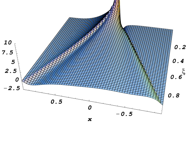
Figure 20: The GPD $H^{u}(x,\xi,t)$ as a function of the longitudinal momentum fraction $x$ and the longitudinal momentum transfer $\xi$ at $t=0$ according to the VGG model. One recognizes for $\xi$=0 the typical shape of a parton distribution (with the sea quarks rising as $x$ goes to 0, the negative $x$ part being interpreted as the antiquark contribution) and as $\xi$ increases the (asymptotic) shape of a distribution amplitude.

One identifies at $\xi=0$ a standard quark density distribution, with the rise around $x=0$ corresponding to the diverging sea contribution. The negative $x$ part is related to antiquarks. One sees the evolution with $\xi$ which tend towards the shape of an asymptotic DA.

3.1.2 The $D$-term

As we saw, GPDs built on the DD ansatz automatically satisfy the polynomiality rule. However, because of the $\delta(x-\beta-\xi\alpha)$ function in Eq. (39), the $n^{th}$ $x$ moment of the so defined GPDs is at most a polynomial in $\xi$ of order $n$, while the polynomiality rule allows for a term with one more power, i.e. a $\xi^{n+1}$ term. This means that the DD decomposition of the GPDs is not complete. The so-called $D$-term, denoted by $D(x/\xi,t)$ has been introduced by C. Weiss and M. Polyakov [79] to take into account this “missing” power $\xi^{n+1}$. It can be decomposed in a Gegenbauer series as :

$$D(z,t)=(1-z^{2})\sum_{\stackrel{{\scriptstyle n=1}}{{n\;odd}}}^{\infty}\;d_{n}(t)\;C_{n}^{3/2}(z),$$ (47)

with $|z|\leq 1$. Since the $D$-term corresponds to a flavor singlet contribution, it receives the same contribution from each quark flavor. One can then define a $D$-term contribution for each quark flavor by dividing by a factor $N_{f}=3$, denoting the number of light quark flavors. Furthermore in Eq. (47), the form factors $d_{1}(t)$, $d_{3}(t)$, … at $t=0$ have been estimated, in a first approach, in the chiral soliton model as [34] : $d_{1}=-4$, $d_{3}=-1.2$ et $d_{5}=-0.4$.

The D-term “lives” only in the $-\xi<x<\xi$ region, i.e. the $q\bar{q}$ part of the GPDs, whence the motivation to expand it on odd Gegenbauer polynomials which are the standard functions on which meson DAs are decomposed. We will come back to the D-term in section 3.4 devoted to dispersion relations.

We are now going to describe the VGG and GK models which are both based on the DD (+ D-term) ansatz for the $(x,\xi)$-dependence and which differ essentially by the parameterization of their $t$-dependence.

3.1.3 The VGG model

The VGG model is associated with a series of publications released between 1999 and 2005 [80, 81, 34, 82]. The first version of the model was published in 1998 but has since then continuously evolved, benefitting from and integrating the work and inputs of several other authors, as the field of GPD grew and improved. We quote here the main publications and associated steps and improvements of the VGG model over the past 10 years :

• In Ref. [80], at first a parameterization of the GPDs via a $\xi$-independent and $t$-factorized ansatz was used. In a concise notation : $H^{q}(x,\xi,t)=q(x)F_{1}^{q}(t)$, $\tilde{H}^{q}(x,\xi,t)=\Delta q(x)G_{A}^{q}(t)$, etc…

• In Ref. [81], the $\xi$-dependence via the Double Distributions (DD) which was discussed in the previous subsection, was introduced in the GPD parameterization. In a concise notation : $H^{q}(x,\xi,t)=H^{q}_{DD}(x,\xi)F_{1}^{q}(t)$, $\tilde{H}^{q}(x,\xi,t)=\tilde{H}^{q}_{DD}(x,\xi)G_{A}(t)$, etc…

• In Ref. [34], the ”$D$-term” ($D$), as suggested by C. Weiss and M. Polyakov [79], was introduced as well as a “Regge-inspired” unfactorized $t$-dependence, which are we are going to detail in the remaining of this subsection. In a concise notation : $H^{q}(x,\xi,t)=H^{q}_{DD}(x,\xi)x^{-\alpha_{1}^{\prime}t}+\frac{1}{N_{f}}D(\frac{x}{\xi})$, $E^{q}(x,\xi,t)=E^{q}_{DD}(x,\xi)x^{-\alpha_{2}^{\prime}t}-\frac{1}{N_{f}}D(\frac{x}{\xi})$, etc…

• In Ref. [82], the Regge dependence was modified so as to satisfy the FF counting rules at large $t$. In a concise notation : $H^{q}(x,\xi,t)=H^{q}_{DD}(x,\xi)x^{-\alpha_{1}^{\prime}(1-x)t}+\frac{1}{N_{f}}D(\frac{x}{\xi})$, $E^{q}(x,\xi,t)=E^{q}_{DD}(x,\xi)(1-x)^{\eta}x^{-\alpha_{2}^{\prime}(1-x)t}-\frac{1}{N_{f}}D(\frac{x}{\xi})$, etc…

One can also complement this list by the work of Ref. [17] in which twist-3 effects are estimated in the Wandura-Wilczek approximation.

1. Parameterization of the GPD $H$
   

   The $t$-dependence of the GPD $H$ in the VGG model is based on Regge theory. In short, Regge theory is based on the general concepts of unitarity and analyticity of scattering amplitudes and states that the high energy behavior of amplitudes should follow a $s^{\alpha(t)}$ behavior, where $s$ is the (squared) center-of-mass energy of the system and $\alpha(t)$ is a Regge trajectory. A Regge trajectory is the relation between the squared mass and the spin of a family of mesons (or baryons) which share the same quantum numbers, except for spin. This high energy property is used, for instance, to determine, by extrapolation, the PDFs into the very small $x$ region (i.e. high $s$ domain since $x\approx\frac{1}{s}$) where no measurement is possible.

   Thus, $q(x)$, which governs the $x$ behavior of the DIS cross section, or, equivalently, of the forward ($t=0$) Compton amplitude, should follow, as $x\to 0$, a $\frac{1}{x^{\alpha(0)}}$ behavior. The leading meson trajectory associated to the valence part $q_{v}(x)$, which corresponds to an isovector combination (i.e. non-singlet), is the isovector vector meson $\rho$ trajectory whose intercept $\alpha_{\rho}(0)=0.5$. The sea (and gluon) part of the PDF $q_{s}(x)$ is an isoscalar (singlet) combination, and the associated trajectory is the Pomeron trajectory, which has the quantum numbers of the vacuum and for which $\alpha_{\wp}(0)=1$. One therefore infers that $q_{v}(x)\approx x^{-0.5}$ and $q_{s}(x)\approx g(x)\approx x^{-1}$ as $x\to 0$ (the trajectories governing the small $x$ behavior of the polarized quark distributions are those of the axial vector mesons).

   For GPDs, i.e. the “non-forward” PDFs, the idea is to generalize this Regge ansatz for non-zero $t$ values. Thus, the first formula which naturally suggests itself, is (for the $H$ GPD and for $\xi=0$, to simplify matter in a first stage) :

   $$H^{q}(x,0,t)=q_{v}(x)x^{-\alpha^{\prime}t}$$ (48)

   with the assumption of a linear Regge trajectory, i.e. : $\alpha(t)=\alpha(0)+\alpha^{\prime}t$. $\alpha^{\prime}$ is a parameter which can be strongly constrained by the sum rules linking the GPDs to the $F_{1}$ (and $F_{2}$) FF(s), following Eq. (11) and, in particular, the nucleon charge radius.

   However, the ansatz of Eq. (48) has the shortcoming that it doesn’t produce a correct behavior of the FFs at large $t$. At large $t$, quark counting rules dictate that $F_{1}(t)$ should behave as $\frac{1}{t^{2}}$. $F_{2}(t)$, which is spin flip, and is therefore suppressed, should behave as $\frac{1}{t^{3}}$. The ansatz of Eq. (48) does not satisfy these limits. Indeed, if $q_{v}(x)\approx(1-x)^{\nu}$ for $x\to 1$, one can show that, at large $\mid t\mid$ :

   $$\int_{0}^{1}(1-x)^{\nu}x^{-\alpha^{\prime}t}dx\propto\frac{1}{\alpha^{\prime}}\,\mid t\mid^{-(\nu+1)}$$ (49)

   which, with $\nu\approx 3$, taken from phenomenology, yields a $1/t^{4}$ asymptotic behavior for $F_{1}(t)$, which is at variance with the $1/t^{2}$ behavior seen in the $F_{1}$ form factor data, and expected from the asymptotic behavior.

   The large-$t$ power behavior of $F_{1}(t)$ should be governed by the large $x$ ($\to 1$) behavior of $q(x)$. Physically, the asymptotic large $t$-domain consists in probing the simplest configuration of the nucleon, i.e. the 3-quark configuration of the nucleon wave function which corresponds to the large $x$ region. The idea is then to modify the large $x$ behavior of Eq. (48). It can be done by introducing a $(1-x)$ term in the exponent of Eq. (48). With:

   $$\int_{0}^{1}(1-x)^{\nu}x^{-\alpha^{\prime}(1-x)t}dx\propto\frac{1}{\alpha^{\prime}}\,\mid t\mid^{-(\nu+1)/2}$$ (50)

   one has, for $\nu\approx 3$, a $\frac{1}{t^{2}}$ behavior at large $t$.

   To summarize, the ansatz for the VGG GPD $H$ is therefore (for $\xi=0$) :

   $$H(x,0,t)=q_{v}(x)x^{-\alpha^{\prime}(1-x)t}.$$ (51)

   Finally, the full $(x,\xi)-t$ correlation is introduced by “folding in” the Regge ansatz for the $(x,t)$ dependence into the DD concept for the $(x,\xi)$ dependence. One then defines Regge-type DDs :

   $$F^{q}(\beta,\alpha,t)=F^{q}(\beta,\alpha,0)\,\beta^{-\alpha^{\prime}(1-\beta)t}$$ (52)

   where $F^{q}(\beta,\alpha,0)$ is given by the form of Eq. (46). To satisfy the polynomiality rule of Eq. (14) for the GPD $H$, is has been shown in Ref. [79] that a $D$-term has to be added. The full $(x,\xi,t)$ dependence for the GPD $H$ in the VGG model then reads :

   $$H^{q}(x,\xi,t) = \int d\alpha d\beta\delta(x-\beta-\xi\alpha)F^{q}(\beta,\alpha,t)$$ (53)

   $$+ \theta(\xi-|x|)\,\frac{1}{N_{f}}D\left(\frac{x}{\xi},t\right),$$

   with $F^{q}(\beta,\alpha,t)$ defined by Eq. (52).

2. Parameterization of the D-term
   

   The $t$-dependence of the $D$-term is unknown. The $D$-term, being odd in $x$, is not at all constrained by the FF sum rules of Eq. (11). VGG adopts a factorized form with a dipole behavior in $t$ with an adjustable mass scale.

3. Parameterization of the GPD $E$
   

   The parameterization of the GPD $E^{q}$, corresponding with a nucleon helicity flip process, is less constrained as we don’t have the DIS constraint for the $x$-dependence in the forward limit.
   One contribution to the GPD $E^{q}$ is however determined through the polynomiality condition, which requires that the $D$-term contribution is cancelled in the combination $H+E$. Therefore it contributes with opposite sign to $H$ and $E$.
   Similarly to Eq. (53) for $H^{q}$, $E^{q}$ is parameterized in the VGG model by adding a double distribution part to the $D$-term as :

   $$E^{q}(x,\xi,t) = E^{q}_{DD}(x,\xi,t)\,-\,\theta(\xi-|x|)\frac{1}{N_{f}}D\left(\frac{x}{\xi},t\right)\,,$$ (54)

   where $E^{q}_{DD}$ is the double distribution part.
   In the forward limit, the DD part reduces to the function $e^{q}(x)\equiv E^{q}_{DD}(x,0,0)$ which is a priori unknown, apart from its first moment :

   $$\int_{-1}^{+1}dx\;e^{q}(x)\,=\,\kappa^{q}\;,$$ (55)

   where $\kappa^{u}$ and $\kappa^{d}$ are the flavor combinations of the nucleon anomalous magnetic moments given by :

   $$\kappa^{u}\,=\,2\,\kappa^{p}\,+\,\kappa^{n}\,=\,1.673\,,\quad\quad\kappa^{d}\,=\,\kappa^{p}\,+\,2\,\kappa^{n}\,=\,-2.033\,.$$ (56)

   For the $x$-dependence of the forward GPD $e^{q}(x)$, a sum of valence and sea-quark parameterization is implemented in VGG, according to Ref. [34] as :

   $$e^{u}(x)\, = \,A^{u}\;u_{val}(x)\;+\;B^{u}\;\delta(x)\,,$$

   $$e^{d}(x)\, = \,A^{d}\;d_{val}(x)\;+\;B^{d}\;\delta(x)\,,$$

   $$e^{s}(x)\, = \,0\;,$$ (57)

   where the parameters $A^{u},A^{d}$ are related to $J^{u},J^{d}$ through the total angular momentum sum rule, which yields :

   $$A^{q}\,=\,{{2\,J^{q}\,-\,M_{2}^{q}}\over{M_{2}^{q_{val}}}}\,,$$ (58)

   and where the parameters $B^{u},B^{d}$ follow from the first moment sum rule Eq. (55) as :

   $$B^{u}\,=\,\kappa^{u}\,-\,2\,A^{u},\quad\quad B^{d}\,=\,\kappa^{d}\,-\,A^{d}.$$ (59)

   Such parameterization allows to use the total angular momenta carried by $u$- and $d$-quarks, $J^{u}$ and $J^{d}$, directly as GPD fit parameters, and can be used to see the sensitivity of hard electroproduction observables on $J^{u}$ and $J^{d}$, as will be shown further on in section 4.
   Starting from the model for the forward distribution $e^{q}(x)$, the $\xi$-dependence of the GPD $E^{q}_{DD}(x,\xi,0)$ is generated through a double distribution $K^{q}(\beta,\alpha,t)$ as :

   $$E^{q}_{DD}(x,\xi,t)\,=\,\int_{-1}^{1}d\beta\ \int_{-1+|\beta|}^{1-|\beta|}d\alpha\ \,\delta(x-\beta-\alpha\xi)\,K^{q}(\beta,\alpha,t)\ \,.$$ (60)

   The double distribution $K^{q}(\beta,\alpha,0)$ is taken in analogy as in Eq. (46), by multiplying the forward distribution $e^{q}(\beta)$ with the same profile function as in Eq. (46) as :

   $$K^{q}(\beta,\alpha,t)=h(\beta,\alpha)\,e^{q}(\beta)\,.$$ (61)

   The parameterization of Eq. (57) yields for the GPD $E^{q}_{DD}(x,\xi,0)$ :

   $$E^{q}_{DD}(x,\xi,0)\, = \,E^{q}_{val}(x,\xi,0)$$

   $$+ \,B^{q}\,\frac{\Gamma(2b+2)}{2^{2b+1}\Gamma^{2}(b+1)}\,{1\over\xi}\,\theta(\xi-|x|)\,\left(1-{{x^{2}}\over{\xi^{2}}}\right)^{b}\,,$$ (62)

   where the first (second) term originates from the valence (sea) contribution to $e^{q}$ respectively in Eq. (57), and where the parameter $b$ is the power entering the profile function.

   For the $t$-dependence of the GPD $E$, the VGG model uses a Regge ansatz, which was constrained in Ref. [82] to provide a fit to the Pauli form factor $F_{2}$. Since the large-$t$ behavior of $F_{2}(t)$ goes steeper than $1/t^{2}$, the Drell-Yan-West relation implies a different large-$x$ behavior of $e^{q}(x)$ compared with $q(x)$. To produce a faster decrease with $t$, a simple ansatz is to multiply $q_{val}(x)$ by an additional factor of the type $(1-x)^{\eta_{q}}$, thus modifying the $x\approx 1$ limit which is the region driving the large-$t$ behavior of $F_{2}(t)$, as we discussed previously. This yields for the valence part :

   $$K^{q}_{val}(\beta,\alpha,t)=h(\beta,\alpha)\,N_{q}\,q_{val}(\beta)(1-\beta)^{\eta_{q}}\,\beta^{-\alpha^{\prime}t}.$$ (63)

   where the normalization constant $N_{q}$ is determined from the anomalous magnetic moment, and where the Regge slope $\alpha^{\prime}$ and the parameter $\eta_{q}$, which determines the large-$x$ behavior of the forward GPD $e^{q}(x)$, are to be determined from a fit to the nucleon Pauli form factor data as. In contrast, the sea-quark cannot been constrained by the $F_{2}$ FF data. It has for simplicity been assumed to have a same $t$-dependence within VGG as for the valence part.

4. Parameterization of the GPD $\widetilde{H}$
   

   For the ($x$,$\xi$)-dependence, the GPD $\widetilde{H}$ is also based on the DD ansatz with the replacement of the unpolarized PDF $q(\beta)$ in Eq. (46) by the polarized PDF $\Delta q(\beta)$, so as to obtain the appropriate forward limit of Eq. (10):

   $$\tilde{F}(\beta,\alpha,0)=h(\beta,\alpha)\Delta q(\beta)$$ (64)

   For the $t$-dependence, in principle, a Regge ansatz similar to the one used for the unpolarized GPDs (Eq. (51)) could be used. However, at this time, given the relatively few experimental constraints from DVCS on this GPD, a $t$-factorized ansatz has been kept:

   $$\tilde{H}(x,\xi,t)=\int d\alpha d\beta\delta(x-\beta-\xi\alpha)\tilde{F}(\beta,\alpha,t)G_{A}(t)/G_{A}(0).$$ (65)

5. Parameterization of the GPD $\widetilde{E}$
   

   Following the argument of Ref. [83, 84], it is parameterized by the pion exchange in the $t$-channel, which, due to the small pion mass, should be a major contribution:

   $$\tilde{E}^{u/p} = -\tilde{E}^{d/p}={1\over 2}\;\tilde{E}^{(3)}_{\pi-pole}\;,$$

   $$\tilde{E}^{(3)}_{\pi-pole}\, = \,\theta(\xi-|x|)\;h_{A}(t)\;{1\over\xi}\;\phi_{as}\left({x\over\xi}\right)\,$$ (66)

   with the asymptotic distribution amplitude $\phi_{as}$ is given by $\phi_{as}(z)=3/4$ $(1-z^{2})$, and $h_{A}(t)$ is the induced pseudo scalar FF of the nucleon. The contribution of Eq. (66) to the $\widetilde{E}$ GPD, corresponding to a meson or $q\bar{q}$ exchange in the $t$-channel, lives only in the $-\xi\leq x\leq\xi$ region and as such, contributes only to the real part of the DVCS amplitude.

In summary, the VGG parameterization is based on very few inputs:

• a choice for the PDF which drives the forward limit. By choosing a PDF parameterization which take into account the evolution equation, a $Q^{2}$-dependence can be introduced in the GPDs.

• the parameters $b_{v}$ and $b_{s}$, which drive the $(x,\xi)$-dependence and which are set to 1 by default.

• the parameters $\alpha^{\prime}$ and $\eta_{q}$ which drive the $t$-dependence. In Ref. [82], the fit to the proton and neutron FF data yielded $\alpha^{\prime}=1.105$ GeV^-2, $\eta_{u}$=1.713 and $\eta_{d}$=0.566.

• the parameters $J_{u}$, $J_{d}$ which control the normalization of the $E$ GPD and which are unknown a priori.

3.1.4 The GK model

The GK parameterization of the GPDs has been developed in the process of fitting the high-energy (low $x$) DVMP data and has been published in a series of articles [85, 86, 87]. There are numerous data available for DVMP and since the same GPDs as for DVCS enter in the DVMP handbag diagram (Fig. 9), strong constraints on the GPD model parameters can be derived, which are not present in VGG.

• In Ref. [85] the DVMP 2-gluon exchange handbag diagram amplitude (Fig. 9-right) was derived for exclusive $\rho^{0}$ and $\phi$ electroproduction on the proton, taking into account some higher-twist corrections (Sudakov suppression and transverse momenta of the quark). The authors proposed a DD-based ansatz for the gluon GPDs and compared their calculation to the HERA data.

• In Ref. [86] the 2-quark exchange handbag diagram amplitude (Fig. 9-left) was added and a DD-based ansatz for the quark GPDs $H^{q}$ and $E^{q}$ was proposed, which we will describe in the following.

• In Ref. [87], exclusive $\pi^{+}$ electroproduction on the proton was investigated, which allowed to derive a parameterization for the $\tilde{H}$ and $\tilde{E}$ GPDs (as well as for the transversity GPD $H_{T}$, which will not discuss here).

Like VGG, the GK model is based on DDs for the $(x,\xi)$-dependence. In VGG, the $b$ exponents in the profile function of Eq. (46) are usually taken as 1 but they are essentially unconstrained and left as free parameters due to the lack of constraint from the DVCS data. In GK, the $b$ parameters are taken as 1 for valence quarks and 2 for sea quaks. This values correspond to the asymptotic behavior of quark and gluon DAs respectively.

For the $t$-dependence, the GK GPD is expressed (at $\xi=0$) as its forward limit multiplied by an exponential in $t$ with a slope depending on $x$ :

$$GPD^{i}(x,\xi=0,t)=GPD^{i}(x,\xi=0,t=0)\,e^{t\,p_{i}(x)}$$ (67)

with a Regge-inspired profile functional form:

$$p_{i}(x)=\alpha_{i}^{\prime}\ln{1/x}+b_{i}.$$ (68)

The label $i$ stands for valence or sea quark flavours, or gluons. Gluon GPDs are in principle taken into account in GK. This is a difference with VGG which takes into account only quark (valence and sea) GPDs. However, since the present review focuses on the valence region and on the leading-twist leading order domain, the gluonic degrees of freedom are not included in the following calculations.

For quark GPDs, Eq. (67) can be rewritten:

$$GPD^{i}(x,t)=q(x)x^{-\alpha^{\prime}t}\,e^{b_{i}t}$$ (69)

in order to better compare to the VGG ansatz of Eq. (51).

The GK $t$-dependence is different from the one of the VGG model in that:

• There is an $x$-independent term in the exponential (associated with the parameter $b_{q}$),

• The $x$-dependence of the $t$-slope has an extra $(1-x)$ factor in VGG (Eq. (51)).

The parameters in Eq. (67) and (68) are determined by the analysis of DVMP data in the kinematical region $\xi\leq 0.1$, $Q^{2}\geq 3\,\textrm{GeV}^{2}$, $W\geq 4\,\textrm{GeV}$ and $-t\leq 0.6\,\textrm{GeV}^{2}$. The data sensitive mostly to the GPD $H$ are available over a wide $Q^{2}$ range, while the existing data which have a higher sensitivity to $E$, $\tilde{H}$, $\tilde{E}$ are available only in a restricted $Q^{2}$ range. Therefore, a $Q^{2}$-dependence on the GPD $H$ is taken into account through the $Q^{2}$ dependence of the PDF used in the DD ansatz [86, 87] (like in VGG) while it is neglected for the $E$, $\tilde{H}$ and $\tilde{E}$ GPDs. It is also ensured that the valence quark GPDs are in agreement with the nucleon form factors at small $t$ and that all GPDs satisfy positivity bounds [47, 90]. We now detail the parameterization of each GPD.

1. Parameterization of the GPD $H$
   

   The forward limit of the GPD $H$ is the usual unpolarized PDF. To allow an analytic evaluation of the resulting GPD, PDFs are expanded on a basis of half-integer powers of $x$:

   $$H^{i}(x,\xi=0,t=0) = x^{-\alpha_{Hi}(0)}(1-x)^{2n_{i}+1}\sum_{j=0}^{3}c_{ij}\,x^{j/2}$$ (70)

   where $i$ represents various quark flavours. The $Q^{2}$-dependent expansion coefficients $c_{ij}=c_{ij}(Q^{2})$ have been obtained from a fit to the CTEQ6M PDFs [88] and are summarized in Ref. [89]. The parameters appearing in the profile functions (67) obey linear Regge trajectories:

   $$\alpha_{Hi}=\alpha_{Hi}(0)+\alpha_{Hi}^{\prime}t.$$ (71)

   It is assumed that $\alpha_{H{\rm sea}}(t)=\alpha_{Hg}(t)$ and $\alpha_{Hg}(0)=1+\delta_{g}$ as seen in the HERA experiments. The expression of the GPD $H$ stemming from the expansion of Eq. (70) is:

   $$H_{i}(x,\xi,t)=e^{b_{Hi}t}\sum_{j=0}^{3}c_{ij}H_{ij}(x,\xi,t)\,.$$ (72)

   where integrals $H_{ij}$ are written down in Ref. [86]. The slopes $b_{Hi}$ are modeled by:

   $$b_{H{\rm val}} = 0\,,$$

   $$b_{H{\rm sea}}=b_{Hg} = 2.58\,\textrm{GeV}^{-2}+0.25\,\textrm{GeV}^{-2}\ln{\frac{m_{N}^{2}}{Q^{2}+m_{N}^{2}}}\,,$$ (73)

   Sea quark GPDs are further simplified [87] as:

   $$H^{u}_{\rm sea} = H^{d}_{\rm sea}=\kappa_{s}H^{s}_{\rm sea}\,,$$

   $${\rm with}\;\;\;\;\;\;\kappa_{s} = 1+0.68/(1+0.52\ln Q^{2}/Q_{0}^{2}).$$ (74)

   The flavor symmetry breaking factor $\kappa_{s}$ possesses a $Q^{2}$-dependence fitted from the CTEQ6m PDFs. The parameters in the previous equations are determined by the HERA $\rho^{0}$ and $\phi$ data.

2. Parameterization of the GPD $E$
   The constraints on $E$ come mostly from the Pauli FF data [90], through the sum rules of Eq. (11). A DD ansatz is also used. $E(x,\xi=0,t=0)$ is parameterized with a classical PDF functional form:

   $$E^{q}_{\rm val}(x,\xi=0,t=0)=\frac{\Gamma(2-\alpha_{\rm val}+\beta^{q}_{\rm val})}{\Gamma(1-\alpha_{\rm val})\Gamma(1+\beta^{q}_{\rm val})}\kappa_{q}x^{-\alpha_{\rm val}}(1-x)^{\beta^{q}_{\rm val}}\,.$$ (75)

   where the ratio of $\Gamma$ functions ensures the correct normalization of E at $t=0$. The fits to the nucleon Pauli form factors performed in Ref. [90] fix the parameters specifying $E$ for valence quarks to $\beta^{u}_{\rm val}=4$ and $\beta^{d}_{\rm val}=5.6$. The trajectory $\alpha_{E{\rm val}}$ and slope parameter $b_{Ei}$ are assumed equal to the corresponding $H$ parameters.

   The GK model of the gluon and sea $E$ GPDs has been given in Ref. [91] following an idea of M. Diehl and W. Kugler [92]. The DD ansatz is used again and the forward limits of the gluonic and strange quark GPDs are parameterized as

   $$E^{s}(\rho,\xi=t=0)=N_{s}\rho^{-1-\delta_{g}}(1-\rho)^{\beta_{Es}}$$ (76)

   using $\beta_{Es}$=7 and the same Regge trajectory as for $H$. The sea is supposed to be flavour-symmetric. The slopes of the residues $b_{Ei}$ are estimated as :

   $$b_{Es}=0.9\,b_{Hg}.$$ (77)

   The normalization $N_{s}$ of $E^{s}$ is fixed from saturating a positivity bound for a certain range of $x$ [91] (which does not allow to fix the sign of $N_{s}$) : $N_{s}=\pm 0.155$.

3. Parameterization of the GPD $\widetilde{H}$
   The Blümlein-Böttcher results [93] are taken to describe the forward limit of $\widetilde{H}^{i}$ [86, 87]. Only $\widetilde{H}^{i}_{\rm val}$ is modeled and constrained by the HERMES data [94, 95]. $\widetilde{H}_{\rm sea}$ is set to zero. In the same spirit as the modeling of GPDs $H$ and $E$, the forward limit $\widetilde{H}^{i}_{\rm val}(x,\xi=0,t=0)$ is written following a DD ansatz and in an analytical expansion, with the following profile function:

   $$\widetilde{H}^{i}_{\rm val}(x,\xi=0,t=0)=\eta_{i}\,A_{i}x^{-\alpha_{\tilde{H}i}(0)}\,(1-x)^{3}\,\sum_{j=0}^{2}\tilde{c}_{ij}\,x^{j}\,,$$ (78)

   where $i=u,d$. The factors $\eta_{u}$ and $\eta_{d}$ guarantee the correct normalization of the first moment of $\widetilde{H}^{i}_{\rm val}$ which is known from $F$ and $D$ values and $\beta$-decay constants $\eta_{u}=0.926\pm 0.014$ and $\eta_{d}=-0.341\pm 0.018$. The normalization factors $A_{u}$ and $A_{d}$ are defined by:

   $$A_{i}^{-1}=B(1-\alpha_{\tilde{H}i},4)\left[\tilde{c}_{i0}+\tilde{c}_{i1}\,\frac{1-\alpha_{\tilde{H}i}}{5-\alpha_{\tilde{H}i}}+\tilde{c}_{i2}\,\frac{(2-\alpha_{\tilde{H}i})(1-\alpha_{\tilde{H}i})}{(6-\alpha_{\tilde{H}i})(5-\alpha_{\tilde{H}i})}\right]\,,$$ (79)

   where $B(a,b)$ is Euler’s beta function. The coefficients $\tilde{c}$ can be found in Ref. [89].

4. Parameterization of the GPD $\widetilde{E}$
   The GPD $\widetilde{E}$ is also determined only for valence quarks. Its sea part is set to 0. As for VGG, its modeling takes into account the pion pole contribution which reads [81, 84]:

   $$\widetilde{E}^{u}_{\rm pole}=-\widetilde{E}^{d}_{\rm pole}=\Theta(|x|\leq\xi)\,\frac{F_{P}(t)}{4\xi}\,\Phi_{\pi}\Big{(}\frac{x+\xi}{2\xi}\Big{)}\,,$$ (80)

   where $F_{P}$ is the pseudoscalar from factor of the nucleon. The pole contribution to the pseudoscalar form factor is written as

   $$F_{P}(t)=-m_{N}f_{\pi}\,\frac{2\sqrt{2}g_{\pi NN}F_{\pi NN}(t)}{t-m_{\pi}^{2}}\,.$$ (81)

   where $m_{\pi}$ denotes the mass of the pion and $g_{\pi NN}\simeq 13.1$ is the pion-nucleon coupling constant, $f_{\pi}$ is the pion decay constant.

   The pion’s distribution amplitude $\Phi_{\pi}$ is taken as:

   $$\Phi_{\pi}(\tau)=6\tau(1-\tau)\,\big{[}1+a_{2}C^{3/2}_{2}(2\tau-1)\big{]}\,.$$ (82)

   with $a_{2}=0.22$ at the initial scale $Q_{0}^{2}=4\,\textrm{GeV}^{2}$. The form factor of the pion-nucleon vertex $F_{\pi NN}$ is described by [87]:

   $$F_{\pi NN}=\frac{\Lambda_{N}^{2}-m_{\pi}^{2}}{\Lambda_{N}^{2}-t}$$ (83)

   with $\Lambda_{N}=0.44\,\textrm{GeV}$. Such a hadronic FF is not present in the VGG parameterization of $\widetilde{E}$.

   A non-pole contribution, which is not present in VGG, is added and modeled in the same way as $H$, $E$ and $\tilde{E}$, i.e. a functional form for the forward limit is assumed, then skewed with a profile function in a DD ansatz. Flavour independence of the Regge trajectory and the slope of the residue are assumed. The forward limit reads [87, 96]:

   $$\widetilde{E}^{q}_{\rm val}(x,\xi=0,t=0)=N_{\tilde{E}}^{q}x^{\alpha_{\tilde{E}}(0)}\,(1-x)^{5}\,.$$ (84)

   The following values for the various parameters involved are $\alpha_{\tilde{E}}(0)$ = 0.48, $\alpha^{\prime}_{\tilde{E}}$ = 0.45, $b_{\tilde{E}}$ = 0.9 GeV^-2, $N^{u}_{\tilde{E}}$ = 14.0 and $N^{d}_{\tilde{E}}$ = 4.0.

3.2 Dual parameterization

3.2.1 Evolution equations and conformal symmetry

By definition, conformal transformations change only the scale of the metric of Minkowski space, and in particular leave the light cone invariant. The whole conformal group admits a particular subgroup, named collinear conformal group, which maps a given light ray onto itself. This is of special relevance for hadron structure functions since in the parton model, hadrons are viewed as a bunch of partons moving fast along a direction on the light cone. It helps classifying fields according to their collinear conformal symmetry properties. For details we refer to the review of Ref. [97].

Although QCD is not a scale invariant theory (it exhibits a spectrum of massive bound states), conformal symmetry is a symmetry of the classical theory when quarks are considered as massless. It is thus relevant for renormalization at leading order since the counter terms satisfy the symmetry properties of the tree-level (classical) Lagrangian. As operators with different quantum numbers (or symmetry properties) do not mix under renormalization, conformal symmetry is a powerful tool to separate operators at leading order.

In particular Gegenbauer polynomials $C^{3/2}_{n}$ parameterize the local conformal operators associated to the twist 2 matrix elements used to define PDFs or GPDs. They diagonalize the ERBL evolution equations that describe the evolution of GPDs in the inner region $-\xi<x<+\xi$ [33, 34, 35, 36, 37, 38] where GPDs probe the presence of quark-antiquark pairs in the nucleon. This is the region of interest when representing GPDs as an infinite series of $t$-channel exchange resonances, as in the case of the dual model, or alternatively of the Mellin-Barnes representation. Therefore expanding GPDs on a series of orthogonal Gegenbauer polynomials $C^{3/2}_{n}$ is an appealing starting point to parameterize GPDs.

3.2.2 Partial wave expansion and CFFs

The dual parameterization of the GPDs is based on a representation of parton distributions as an infinite series of $t$-channel exchanges [98]. For the unpolarized GPDs, one defines electric ($H^{E}$) and magnetic ($H^{M}$) GPD combinations :

$$H^{(E)}(x,\xi,t) = H(x,\xi,t)+\frac{t}{4m_{N}^{2}}E(x,\xi,t),$$ (85)

$$H^{(M)}(x,\xi,t) = H(x,\xi,t)+E(x,\xi,t),$$ (86)

which are suitable for a $t$-channel partial-wave expansion, which read for the singlet combinations as [99]:

$$H^{(E)}_{+}(x,\xi,t) = 2\sum_{n=1\atop\rm{odd}}^{\infty}\sum_{l=0\atop\rm{even}}^{n+1}B_{nl}^{(E)}(t)\theta\left(1-\frac{x^{2}}{\xi^{2}}\right)\left(1-\frac{x^{2}}{\xi^{2}}\right)C_{n}^{\frac{3}{2}}\left(\frac{x}{\xi}\right)P_{l}\left(\frac{1}{\xi}\right),$$

$$H^{(M)}_{+}(x,\xi,t) = 2\sum_{n=1\atop{\rm odd}}^{\infty}\sum_{l=0\atop{\rm even}}^{n+1}B_{nl}^{(M)}(t)\theta\left(1-\frac{x^{2}}{\xi^{2}}\right)\left(1-\frac{x^{2}}{\xi^{2}}\right)C_{n}^{3/2}\left(\frac{x}{\xi}\right)\frac{1}{\xi}P^{\prime}_{l}\left(\frac{1}{\xi}\right),$$

where $C_{n}^{3/2}(z)$ are the Gegenbauer polynomials, $P_{l}(z)$ are Legendre polynomials, and $B_{nl}(t)$ are generalized form factors. Note that for $H_{+}^{(E)}$ intermediate states with $l^{PC}=0^{++},2^{++},...$ contribute, whereas for $H_{+}^{(M)}$ intermediate states with $l^{PC}=2^{++},4^{++},...$ contribute.

As stated before, the expansion onto a basis of Gegenbauer polynomials allows a trivial solution of the QCD evolution equations at leading order: The $Q^{2}$-evolution of the generalized form factors $B_{nl}(t,Q^{2})$ reads [105]:

$$B_{nl}(t,Q^{2})=B_{nl}(t,Q_{0}^{2})\left(\frac{\ln Q_{0}^{2}/\Lambda^{2}}{\ln Q^{2}/\Lambda^{2}}\right)^{\frac{\gamma_{n}}{\beta_{0}}},$$ (89)

with $\beta_{0}=11-\frac{2}{3}n_{f}$ and:

$$\gamma_{n}=\frac{4}{3}\left(3+\frac{2}{n(n+1)}-4\big{(}\Psi(n+1)+\gamma_{E}\big{)}\right),$$ (90)

where $\Psi$ denotes the Digamma function and $\gamma_{E}$ the Euler-Mascheroni constant.

At fixed $x$ and $\xi$ the series on the rhs of Eqs. (LABEL:eq:duale, LABEL:eq:dualm) are divergent: the sums $H^{(E)}_{+}$ and $H^{(M)}_{+}$ have a support $-1<x<+1$ while each term of the expansions have a support $-\xi<x<+\xi$. However, these formal series can be recast onto convergent Gegenbauer polynomial expansions. For example the electric singlet GPD reads [100]:

$$H^{(E)}_{+}(x,\xi,t)=2(1-x^{2})\sum_{n=1\atop{\rm odd}}^{\infty}A_{n}(\xi,t)C_{n}^{3/2}(x).$$ (91)

The coefficients $A_{n}$ are defined by:

$$A_{n}(\xi,t) = -\frac{2n+3}{(n+1)(n+2)}\sum_{p=1\atop{\rm odd}}^{n}\xi R_{np}(\xi)\frac{(p+1)(p+2)}{2p+3}\sum_{l=0\atop{\rm even}}^{p+1}B_{pl}(t)P_{l}\left(\frac{1}{\xi}\right).$$

Here $R_{np}(\xi)$ is a polynomial of degree $n$:

$$R_{np}(\xi) = \frac{(-1)^{\frac{n+p}{2}}\Gamma\left(\frac{3}{2}+\frac{n+p}{2}\right)}{\Gamma\left(\frac{n-p}{2}+1\right)\Gamma\left(\frac{3}{2}+p\right)}\xi^{p}\vphantom{.}_{2}F_{1}\left(\frac{p-n}{2},\frac{3}{2}+\frac{n+p}{2},\frac{5}{2}+p,\xi^{2}\right),$$ (93)

with $\vphantom{.}{}_{2}F_{1}$ the Gauss hypergeometric function. The convergent expression (91) has been used explicitely for fitting in a truncated form as explained in Sec. 4.2.3.

The procedure to sum the formal series of Eqs. (LABEL:eq:duale, LABEL:eq:dualm) over orbital momentum $l$ through analytical continuation was originally outlined in Ref. [100]. We briefly discuss this in the following for the function $H_{+}^{(E)}$ and for simplicity drop the superscript $(E)$. For an analogous discussion of $H^{(M)}$, as well as the polarized GPDs $\tilde{H}$ and $\tilde{E}$, we refer the reader to Ref. [99].

In order to sum the formal series of Eq. (LABEL:eq:duale), a set of generating functions $Q_{2\nu}(x,t)$ ($\nu=0,1,...$) are introduced, whose Mellin-Barnes moments yield the generalized form factors $B_{nl}(t)$ as [100]:

$$B_{n\,n+1-2\nu}(t)=\int_{0}^{1}dxx^{n}Q_{2\nu}(x,t).$$ (94)

The functions $Q_{2\nu}(x,t)$ are forward-like because at leading order (LO), their scale dependence is given by the standard DGLAP evolution equation, so that these functions behave as usual parton distributions under QCD evolution. Furthermore, the function $Q_{0}(x,t=0)$ is directly related to the parton densities $q(x)$ measured in DIS [100]:

$$Q_{0}(x,t=0)=\left[q+\bar{q}\right](x)-\frac{x}{2}\int_{x}^{1}\frac{dz}{z^{2}}\ \left[q+\bar{q}\right](z)\,.$$ (95)

The usefulness of the dual parameterization originates when expanding the GPD around $\xi=0$. The functions with higher $\nu$ are more suppressed for small values of $\xi$. An expansion with $x$ fixed to the order $\xi^{2\nu}$ involves only a finite number of functions $Q_{2\mu}(x,t)$ with $\mu\leq\nu$.

Within the dual parameterization for the GPDs, the CFFs entering hard exclusive observables can be expressed in terms of forward-like functions. For the combination of the CFF of Eqs. (19, 20), corresponding with the electric GPD of Eq. (85), this is given by [100, 101]:

$$H_{Im}+\frac{t}{4m_{N}^{2}}E_{Im} = \frac{2}{\pi}\int\limits_{\frac{1-\sqrt{1-\xi^{2}}}{\xi}}^{1}\frac{dx}{x}N^{(E)}(x,t)\ \Biggl{[}\frac{1}{\sqrt{2x/\xi-x^{2}-1}}\Biggr{]}\,,$$ (96)

$$H_{Re}+\frac{t}{4m_{N}^{2}}E_{Re} = -2\int\limits_{0}^{\frac{1-\sqrt{1-\xi^{2}}}{\xi}}\frac{dx}{x}N^{(E)}(x,t)$$ (97)

$$\times\Biggl{[}\frac{1}{\sqrt{1-2x/\xi+x^{2}}}+\frac{1}{\sqrt{1+2x/\xi+x^{2}}}-\frac{2}{\sqrt{1+x^{2}}}\Biggr{]}$$

$$- 2\int\limits_{\frac{1-\sqrt{1-\xi^{2}}}{\xi}}^{1}\frac{dx}{x}N^{(E)}(x,t)\ \Biggl{[}\frac{1}{\sqrt{1+2x/\xi+x^{2}}}-\frac{2}{\sqrt{1+x^{2}}}\Biggr{]}$$

$$- \frac{4}{N_{f}}D(t)\,,$$

where $N_{f}=3$ and where the $D$-form factor is obtained from the $D$-term of Eq. (47) as :

$$D(t)=\sum_{n=1}^{\infty}d_{n}(t).$$ (98)

Furthermore, in Eqs. (96, 97), the function $N^{(E)}(x,t)$ is defined as :

$$N^{(E)}(x,t)=\sum_{\nu=0}^{\infty}x^{2\nu}\ Q^{(E)}_{2\nu}(x,t)\,.$$ (99)

Analogous relations are obtained of the magnetic GPD combination $H^{(M)}$ of Eq. (86) in terms of a function $N^{(M)}$ which is a sum of forward-like functions $Q^{(M)}_{2\nu}$. The amplitude within the dual parameterization of GPDs, given by Eqs. (96, 97), automatically satisfies a dispersion relation, with the subtraction constant given by the $D$-FF [101]. We will discuss the general dispersion relation approach for the DVCS amplitude in more detail in Section 3.4.

The information contained in the LO DVCS amplitude is in one-to-one correspondence with the knowledge of the functions $N(x,t)$ and the $D$-FF $D(t)$, because Eq. (96) can be inverted [101], i.e. the functions $N$ can be expressed unambiguously in terms of integrals over $\xi$ of $H_{Im}$ and $E_{Im}$. This inversion corresponds to the Abel transform tomography [102], for details see Ref. [101, 103]. This equivalence implies that the function $N(x,t)$ contains the maximal information about GPDs that is possible to obtain from the observables. Another important feature of the expressions (96, 97) for the amplitude is that one can easily single out the contributions to the amplitude coming from the forward parton densities. Indeed, the first term in the sum (99) is given by the function $Q_{0}$ which is related to the ($t$-dependent) parton densities by Eq. (95). The advantage of the dual parameterization is that one can clearly separate the contribution of the ($t$-dependent) parton densities from genuine non-forward effects encoded in the functions $Q_{2},Q_{4},\dots$.

3.2.3 Modeling the forward functions

A number of phenomenological studies of DVCS observables have been made using the dual parameterization. Most prominently, studies involving only the forward function $Q_{0}$ have been made. In such a minimal model, the $x$ dependence is parameter free as it is completely fixed by the forward parton distributions, merely leaving the $t$ dependence of the GPD to be modeled. One typically uses a Regge motivated model to correlate the $x$ and $t$-dependence of the function $Q_{0}(x,t)$, analogous as it was discussed above for the double distribution model.

Such a minimal model was found to overpredict the data at small and intermediate $x_{B}$: Ref. [104, 105, 106] found that DVCS experiments at HERA (HERMES) were overpredicted by roughly a factor of 2 (1.5) respectively. At larger values of $x_{B}$, for DVCS experiments at JLab@6GeV, it was shown that the bulk effect of the DVCS beam helicity cross section difference can be understood within such a minimal dual model [108], which we show in more detail below.

To improve on the description, especially at smaller values of $x_{B}$, within the dual parameterization requires to go beyond the minimal model by keeping more generating functions $Q_{2},Q_{4},...$, and extend to the next-to-leading order accuracy. A first step to model the functions $Q_{2}$ and $Q_{4}$ has been made using a nonlocal chiral quark model [107] or by extracting them from comparison with the double distribution parameterization [99].

For a comparison with data in the valence, we will be using a model for the LO forward-like functions $Q_{0}^{(E)}$ and $Q_{0}^{(M)}$ as [109] :

$$Q_{0}^{(E)}(x,t) = \left[q_{+}(x,t)+\frac{t}{4m^{2}}e_{+}(x,t)\right]$$ (100)

$$- \frac{x}{2}\int_{x}^{1}\frac{dz}{z^{2}}\left[q_{+}(z,t)+\frac{t}{4m^{2}}e_{+}(z,t)\right],$$

$$Q_{0}^{(M)}(x,t) = \frac{1}{2}\int_{x}^{1}\frac{dz}{z}\left[q_{+}(z,t)+e_{+}(z,t)\right]\left(1+\frac{x}{z}\right),$$ (101)

For the forward GPD $H_{+}(x,0,t)\equiv q_{+}(x,t)$, we use a Regge type ansatz :

$$q_{+}(x,t)=q_{+}(x)\,x^{-\alpha^{\prime}t},$$ (102)

with $\alpha^{\prime}=1.105$ GeV^-2 fixed from the form factor sum rule [82]. For the forward GPD $E_{+}(x,0,t)\equiv e_{+}(x,t)$, we use an ansatz by expressing the magnetic GPD $q_{+}+e_{+}$ as a Mellin convolution of $q_{+}$ with a kernel function, modeled as :

$$q_{+}(x,t)+e_{+}(x,t)=\int_{x}^{1}\frac{dz}{z}q_{+}(z,t)\,C\left(\frac{x}{z}\right)^{\alpha}\left(1-\frac{x}{z}\right)^{\beta},$$ (103)

where $C$ is a constant, which is to be determined from the second moments of the GPDs.

The second moment of the forward parton distribution $q_{+}$ at $t=0$ yields the total momentum carried by quarks and anti-quarks :

$$M^{q}_{2}=\int_{0}^{1}dxxq_{+}(x,0),$$ (104)

whereas the second moment of the magnetic GPD combination $(q_{+}+e_{+})$ at $t=0$ yields the total quark angular momentum :

$$2J^{q}=\int_{0}^{1}dxx\left[q_{+}(x,0)+e_{+}(x,0)\right].$$ (105)

Eqs. (104, 105) then allow to express the constant $C$ as :

$$C=\frac{2J^{q}}{M^{q}_{2}}\frac{\Gamma(\alpha+\beta+3)}{\Gamma(\alpha+2)\Gamma(\beta+1)}.$$ (106)

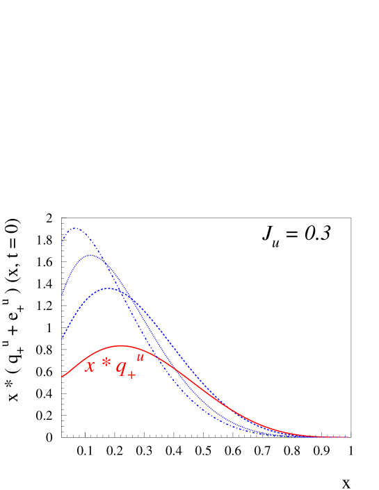
Figure 21: Parameterization for the forward function $(q_{+}^{u}+e_{+}^{u})(x,t=0)$ for $J_{u}=0.3$, and for different values of $\alpha,\beta$ : $\alpha=0$, $\beta=0$ (dashed-dotted curve); $\alpha=1$, $\beta=0$ (dotted curve); $\alpha=2$, $\beta=-0.5$ (dashed curve). The solid curve shows the parameterization for the forward function $q_{+}^{u}(x,t=0)$.

3.3 Mellin-Barnes parameterization of GPDs

3.3.1 Partial wave expansion

In this section, we will discuss the Mellin-Barnes parameterization of GPDs described in the works of  [113, 114]. For simplicity, we do not write the dependence of GPDs on the momentum transfer $t$. The method is based on making a partial-wave expansion of GPDs. It is analogous in spirit to the dual model partial wave expansion explained in Sec. 3.2, although both representations differ on the resummation of this expansion.

In order to recover the Mellin moments of PDFs when taking the forward limit of conformal moments of GPDs, one rescales the Gegenbauer polynomials to define the polynomials $c_{n}(x,\xi)$:

$$c_{n}(x,\xi)=\frac{\Gamma\left(\frac{3}{2}\right)\Gamma(n+1)}{2^{n}\Gamma\left(\frac{3}{2}+n\right)}\,\xi^{n}C^{3/2}_{n}\left(\frac{x}{\xi}\right),$$ (107)

for any integer $n$. Conformal moments $F_{n}(\xi)$ of a GPD $F$ ($F$ = $H$, $E$, $\tilde{H}$ or $\tilde{E}$) are then defined by:

$$F_{n}(\xi)=\int_{-1}^{+1}dx\,c_{n}(x,\xi)F(x,\xi).$$ (108)

The polynomiality of GPDs ensures that $F_{n}$ is a polynomial in $\xi$ of degree at most $n+1$. The rescaled polynomials are orthogonal to the polynomials $p_{n}$ defined by:

$$p_{n}(x,\xi)=\frac{1}{\xi^{n+1}}\theta\left(1-\frac{x^{2}}{\xi^{2}}\right)\left(1-\frac{x^{2}}{\xi^{2}}\right)\frac{2^{n}\Gamma\left(\frac{5}{2}+n\right)}{\Gamma\left(\frac{3}{2}\right)\Gamma(3+n)}(-1)^{n}C^{3/2}_{n}\left(\frac{x}{\xi}\right).$$ (110)

The conformal partial wave expansion then reads:

$$F(x,\xi)=\sum_{n=0}^{\infty}(-1)^{n}p_{n}(x,\xi)F_{n}(\xi).$$ (111)

This is the common basis of the dual and Mellin-Barnes representations. The left-hand-side of Eq. (111) has support $x\in[-1,+1]$ and the right-hand-side has support $x\in[-\xi,+\xi]$. Therefore for $|\xi|<1$ this sum has to be divergent and can be understood as a formal definition of conformal moments. It can be resummed by means of the Sommerfeld - Watson transform [115]:

$$F(x,\xi)=\frac{1}{2i}\int_{\mathcal{C}}dj\,\frac{1}{\sin\pi j}p_{j}(x,\xi)F_{j}(\xi),$$ (112)

where $\mathcal{C}$ is a contour in the complex plane enclosing all non-negative integers (which are the poles of $j\mapsto 1/\sin\pi j$ with residues $(-1)^{j}/\pi$). At this stage, it is only assumed that the analytic continuations of the functions $p_{n}$ and of the moments $F_{n}$ have no singularities inside the contour $\mathcal{C}$. Using the residue theorem one relates Eq. (112) to Eq. (111). Since the analytic continuation of a function of a discrete variable is not unique, this is a non-trivial step. A justification for it is given below.

Using such analytic continuations $p_{j}$ and $F_{j}$, one can deform the integration contour $\mathcal{C}$ so that all singularities of conformal moments lie left to a straight line parallel to the imaginary axis. If the integrand of Eq. (114) decreases fast enough at infinity, one obtains:

$$F(x,\xi)=\frac{1}{2i}\int_{c-i\infty}^{c+i\infty}dj\,\frac{1}{\sin\pi j}p_{j}(x,\xi)F_{j}(\xi),$$ (113)

where the real $c$ constant is suitably chosen. This large-$j$ behavior is another condition that should be fulfilled by the analytic continuations $p_{j}$ and $F_{j}$.

The analytic continuation of $p_{n}$ can be expressed in terms of hypergeometric $\hphantom{}{}_{2}F_{1}$ and gamma $\Gamma$ functions:

$$p_{j}(x,\xi)=\theta(\xi-|x|)\frac{1}{\xi^{j+1}}P_{j}\left(\frac{x}{\xi}\right)+\theta(x-\xi)\frac{1}{\xi^{j+1}}Q_{j}\left(\frac{x}{\xi}\right),$$ (114)

where:

$$P_{j}\left(\frac{x}{\xi}\right) = \frac{2^{j+1}\Gamma\left(\frac{5}{2}+j\right)}{\Gamma\left(\frac{1}{2}\right)\Gamma(1+j)}(1+x)\hphantom{}_{2}F_{1}\left(-(j+1),j+2,2,\frac{\xi+x}{2\xi}\right),$$ (115)

$$Q_{j}\left(\frac{x}{\xi}\right) = -\frac{\sin\pi j}{\pi}\hphantom{}_{2}F_{1}\left(\frac{j+1}{2},\frac{j+2}{2},\frac{5}{2}+j,\frac{\xi+x}{2\xi}\right).$$ (116)

However the explicit calculation of the analytic continuation of conformal moments for any value of $\xi$ and any GPD model fulfilling the aforementioned conditions is an intricate mathematical question. An explicit general procedure is nevertheless described in the case $|\xi|\leq 1$ in Ref. [114].

3.3.2 Compton Form Factors in the Mellin-Barnes representation

To simplify the discussion we restrict ourselves to the case of the singlet GPD $H_{+}$ and its associated CFF defined in Eq. (28). Inserting the Mellin-Barnes representation (113) for the GPD $H$ and permuting the integrals over $x$ and $j$, the CFF $\mathcal{H}(\xi,Q^{2})$ reads:

$$\mathcal{H}(\xi,Q^{2})=\frac{1}{2i}\int_{c-i\infty}^{c+i\infty}dj\,\frac{1}{\xi^{j+1}}\left[i+\tan\left(\frac{\pi j}{2}\right)\right]\left[C^{0}_{j}+\ldots\right]H_{j}(\xi,\mu^{2}),$$ (117)

where we indicated the hard scale $Q^{2}$ explicitly. Furthermore, the coefficients $C^{0}_{j}$ are the conformal moments of the hard scattering kernel $C^{+}$, and the dots refer to NLO terms proportional to $\alpha_{s}$. Since we will discuss LO results, we only quote the expression for $C^{0}$ (for results at NLO, see Ref. [114]):

$$C^{0}_{j}=\frac{2^{j+1}\Gamma\left(\frac{5}{2}+j\right)}{\Gamma\left(\frac{3}{2}\right)\Gamma(3+j)}.$$ (118)

Evolution of GPDs can be included as well in this formalism, taking the conformal moment $(C\otimes E)_{j}$ of the convolution of hard scattering $C$ and evolution $E$ operators.

3.3.3 Modeling of GPD conformal moments

In the spirit of the dual model, the conformal moments of GPDs can be viewed as the result of $t$-channel exchanges of resonances $R_{J}$ with angular momentum $J$, taking into account an effective $\gamma^{*}\gamma R_{J}$ vertex $h_{J}$, a propagator with an effective Regge pole $\alpha(t)$ and a smooth profile for the distribution amplitude of $R_{J}$:

$$H_{j}(\xi,t)=\sum_{J}^{j+1}H_{J,j}\frac{1}{J-\alpha(t)}\frac{1}{\left(1-\frac{t}{M^{2}}\right)^{p}}\xi^{j+1-J}d_{0,\nu}^{J}(\xi)$$ (119)

where Wigner’s $SO(3)$ functions [117] are denoted $d_{0,\nu}$ where $\nu=0$ or $\nu=\pm 1$ depending on hadron helicities. They involve Legendre polynomials when $\nu=0$ (electric GPD combination of Eq. (85)) and derivative of Legendre polynomials when $|\nu|=1$ (magnetic GPD combination of Eq. (86)).

Such modeling of conformal moments has been used in Ref. [113] to fit to unpolarized DVCS data at small $x_{B}$ at LO, NLO (in the $\overline{\textrm{MS}}$ and $\overline{\textrm{CS}}$ schemes) and NNLO (in the $\overline{\textrm{CS}}$ scheme).

3.3.4 Modeling of the GPD $H(\xi,\xi,t)$ within the quark spectator model

With a DD representation and a $t$-dependence inspired from a quark spectator model, the following functional form for the GPD $H$ is used for fitting:

$$H(\xi,\xi,t)=\frac{nr}{1+\xi}\left(\frac{2\xi}{1+\xi}\right)^{-\alpha(t)}\left(\frac{1-\xi}{1+\xi}\right)^{b}\frac{1}{\left(1-\frac{1-\xi}{1+\xi}\frac{t}{M^{2}}\right)^{p}}$$ (120)

where the parameters $n$, $\alpha(t)$ and $p$ are a priori known. In the valence case these parameters are deduced from Regge $\omega$ and $\rho$ trajectories and PDF parameterization. In the sea case, the parameterization (120) is requested to reproduce the small $x_{B}$ fits in the Mellin-Barnes representation.

LO dispersion relations (see next section) are implemented by means of a $t$-dependent subtraction constant parameterized with a normalization constant $C$ and a mass scale $M_{C}$:

$$D(t)=C\left(1-\frac{t}{M_{c}^{2}}\right)^{2}.$$ (121)

For the valence part, this leaves thus five free parameters to fit data: $M$ (valence), $b$ (valence), $r$ (valence) which respectively control the $t$-dependence, the large $x$ behavior and the skewdness effect of the valence part of $H$, and $C$ and $M_{C}$ which respectively control the normalization and $t$-dependence of the D-term. One can use an ansatz similar to Eq. 120 for $\tilde{H}$ which introduces three additional parameters $\tilde{M}$, $\tilde{b}$ and $\tilde{r}$. We come back to this in Section 4.1.4.

3.4 Dispersion relation approach to DVCS: general formalism

As has been discussed in Section 2, the observables entering DVCS are the CFFs, which depend on the GPDs. The CFFs correspond with the real and imaginary parts of the DVCS amplitudes, as given by Eqs. (19 - 26). At a fixed value of the momentum transfer $t$ and the external virtuality $Q^{2}$, the analyticity of the virtual Compton amplitude in the energy variable $\nu$ (or equivalently in the variable $\xi$) allows to write down general dispersion relations, which relate these real and imaginary parts. The different GPD models and parameterizations detailed above are specific ways to implement such dispersion relations. In particular, the double distribution, dual, and Mellin-Barnes parameterizations all satisfy the general dispersion relation for the twist-2 DVCS amplitude which we will detail below.

When making contact with data, the dispersion relation (DR) approach is a very useful tool as it allows to put additional constraints on the data by relating different observables. For the non-forward virtual Compton scattering (VCS) on a nucleon, described by a spacelike incoming photon and a real outgoing photon, the general dispersive framework for the 12 independent invariant amplitudes has been developed in Ref. [118]. Such a framework has been successfully applied to VCS data in the region around threshold and into the first nucleon resonance region, and allowed to extract low-energy constants, proportional to nucleon polarizabilities from VCS data, see Ref. [119] for a review and details.

When describing DVCS data, one may also use the dispersive techniques to put additional constraints on GPD parameterizations of the CFFs. For the twist-2 DVCS amplitude, the dispersive framework for the DVCS amplitude has been discussed in a number of different works, see Refs. [120, 121, 101, 122, 108, 123]. We will discuss here the use of DRs for the DVCS amplitude in some detail for the GPD $H$. Subsequently, we will briefly discuss the amplitudes involving the other GPDs.

We denote the DVCS amplitude which involves the GPD $H$ by $A(\xi,t)$ :

$$A(\xi,t)\equiv-\int_{0}^{1}\,dx\,H_{+}(x,\xi,t)\left[\frac{1}{x-\xi+i\varepsilon}+\frac{1}{x+\xi-i\varepsilon}\right],$$ (122)

which depends on the GPD singlet combination $H_{+}$ defined in Eq. (29). The real and imaginary parts of the amplitude $A(\xi,t)$ are related to the CFF introduced in Eq. (28), as :

$$A(\xi,t) = -{\cal H}(\xi,t).$$ (123)

To write down DRs, we start by introducing the kinematic (energy) variables :

$$\nu=\frac{Q^{2}}{2m\xi},\quad\quad\nu^{\prime}=\frac{Q^{2}}{2mx},$$ (124)

which allow to define amplitudes which are either even or odd in $\nu$. Denoting the DVCS amplitude depending on $\nu$ and $t$ by $\bar{A}(\nu,t)$, the unpolarized DVCS amplitude is even in $\nu$, i.e.:

$$\bar{A}(\nu,t)=\bar{A}(-\nu,t).$$ (125)

We can then write down a once-subtracted DR for the amplitude $\bar{A}$ (assuming one subtraction is enough to make it convergent) as :

$$Re\bar{A}(\nu,t)=\bar{A}(0,t)+\frac{\nu^{2}}{\pi}{\cal P}\int_{\nu_{0}}^{\infty}\frac{d{\nu^{\prime}}^{2}}{{\nu^{\prime}}^{2}}\frac{Im\bar{A}(\nu^{\prime},t)}{{\nu^{\prime}}^{2}-\nu^{2}},$$ (126)

where a subtraction has been made at $\nu=0$, and where $\nu_{0}=Q^{2}/2m_{N}$ corresponds to the elastic threshold. Using Eq. (124), we can rewrite Eq. (126) in a DR in the variable $\xi$ as :

$$ReA(\xi,t)=\Delta(t)+\frac{2}{\pi}{\cal P}\int_{0}^{1}\,\frac{dx}{x}\,\frac{ImA(x,t)}{\left(\xi^{2}/x^{2}-1\right)},$$ (127)

or equivalently

$$ReA(\xi,t)=\Delta(t)-{\cal P}\int_{0}^{1}\,dx\,H_{+}(x,x,t)\left[\frac{1}{x-\xi}+\frac{1}{x+\xi}\right],$$ (128)

where the subtraction term (at zero energy) is denoted by $\Delta(t)$. One notices that in contrast to the convolution integral entering the real part of the CFF in Eq. (123), where the GPD enters for unequal values of its first and second argument, the integrand in the DR (spectral function) corresponds to the GPD where its first and second arguments are equal. Combining Eqs. (122) and (128) allows to re-express the subtraction term as:

$$\Delta(t)={\cal P}\int_{0}^{1}\,dx\,\left[H_{+}(x,\xi,t)-H_{+}(x,x,t)\right]\left[\frac{1}{\xi-x}-\frac{1}{\xi+x}\right],$$ (129)

which is independent of $\xi$. When formally taking $\xi=0$ in Eq. (129) and use time reversal invariance : $H(x,-x,t)=H(x,x,t)$ to convert from the singlet GPD $H_{+}$ to the GPD $H$, one arrives at the sum rule:

$$\Delta(t)=-2\;\int_{-1}^{1}\,dx\,\frac{1}{x}\left[H(x,0,t)-H(x,x,t)\right].$$ (130)

As pointed out in Ref. [124], since both $H(x,0,t)/x$ and $H(x,x,t)/x$ are even functions of $x$, their singularities cannot be regularized by the principle value prescription, and there are no indications that the singularities of both functions cancel each other. However, it was shown [124] that the validity of the sum rule of Eq. (130) can be demonstrated by decomposing the GPD into a double distribution ($H_{DD}$) part and a D-term $(H_{D})$ part. The 1/x integrals of the $H_{DD}$ parts (plus distributions) do not contribute to the sum rule of Eq. (130). The D-term parts are proportional to a $\delta$-function in $x$ as:

$$\frac{H_{D}(x,0,t)}{x} = \delta(x)\,\frac{1}{N_{f}}\,\int_{-1}^{1}dz\frac{D(z,t)}{z}\,,$$

$$\frac{H_{D}(x,x,t)}{x} = \delta(x)\,\frac{1}{N_{f}}\,\int_{-1}^{1}dz\frac{D(z,t)}{z(1-z)}\,,$$ (131)

where $D(z,t)$ is the D-term, see Eq. (47). Using Eq. (131), one then obtains for the sum rule of Eq. (130):

$$\Delta(t)\equiv\frac{2}{N_{f}}\int_{-1}^{1}dz\,\frac{D(z,t)}{1-z}.$$ (132)

We thus observes that the subtraction term entering the DR for the DVCS amplitude $A$ is directly proportional to the D-term form factor. It can be obtained from the Gegenbauer expansion of the $D$-term, Eq. (47), as:

$$\Delta(t)=\frac{4}{N_{f}}\sum_{\stackrel{{\scriptstyle n=1}}{{n\;odd}}}^{\infty}\;d_{n}(t).$$

In practise, one can evaluate the dispersion integral in Eq. (128) by the ordinary integral:

$$ReA(\xi,t) = \Delta(t)-\int_{0}^{1}\,dx\,\left\{H_{+}(x,x,t)-H_{+}(\xi,\xi,t)\right\}\left[\frac{1}{x-\xi}+\frac{1}{x+\xi}\right]$$ (133)

$$- H_{+}(\xi,\xi,t)\ln\left(\frac{1-\xi^{2}}{\xi^{2}}\right),$$

which is easy to implement in a numerically stable way. Note that for the case where $H(x,x,0)\sim 1/x$ for $x\to 0$, the singularity cancels out of the integral.

For the CFF involving the GPD $E$, one can write down an analogous sum rule as for $H$. In this case, the subtraction function is given by $-\Delta(t)$, as the $D$-form factor drops out in the sum of $H+E$.

Analogous to the unpolarized DVCS amplitude, which is even in $\nu$, one can also write down a DR for the polarized DVCS amplitude, which involves the GPD $\tilde{H}$, and which is odd in $\nu$ :

$$\bar{A}(\nu,t)=-\bar{A}(-\nu,t).$$ (134)

Assuming an unsubstracted DR for the odd amplitude, allows to write :

$$Re\bar{A}(\nu,t)=\frac{2\nu}{\pi}{\cal P}\int_{\nu_{0}}^{\infty}\,d\nu^{\prime}\frac{Im\bar{A}(\nu^{\prime},t)}{{\nu^{\prime}}^{2}-\nu^{2}}.$$ (135)

Denoting the polarized DVCS amplitude, depending on $\xi$ and $t$ by $\tilde{A}(\xi,t)$, the DR then reads :

$$Re\tilde{A}(\xi,t)=-\frac{1}{\pi}{\cal P}\int_{0}^{1}\,dx\,Im\tilde{A}(x,t)\left[\frac{1}{x-\xi}-\frac{1}{x+\xi}\right],$$ (136)

with

$$Im\tilde{A}(x,t) = \pi\,\tilde{H}_{+}(x,x,t),$$ (137)

with the polarized singlet GPD $\tilde{H}_{+}$ defined as in Eq. (30).

In Figs. 22 and 23, we show a DR evaluation of the DVCS amplitude corresponding with the GPDs $H$ and $E$ respectively, within both DD and dual parameterizations.

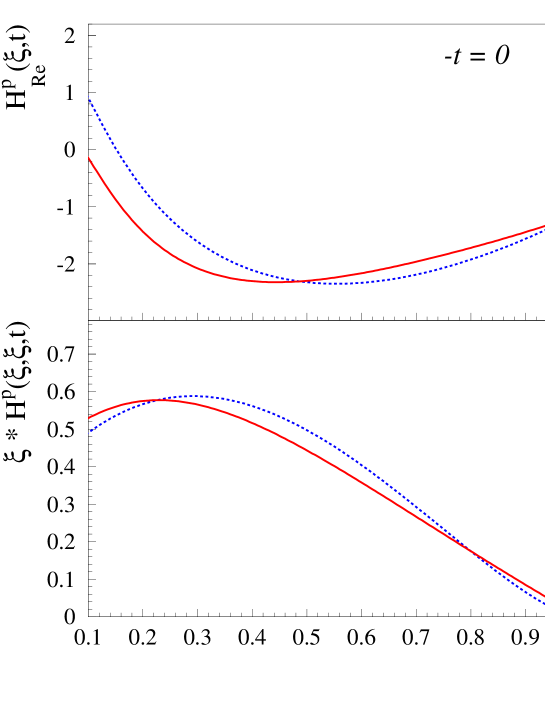
Figure 22: Comparison of the real and imaginary parts of the CFF related with the GPD $H$ for the proton at $t=0$, excluding the $D$-FF subtraction term. The DD parameterization for $b_{val}=b_{sea}=1$ is shown by the solid red curves. The dual parameterization based on the forward function $Q_{0}$, Eq. (95), is shown by the dashed blue curves.

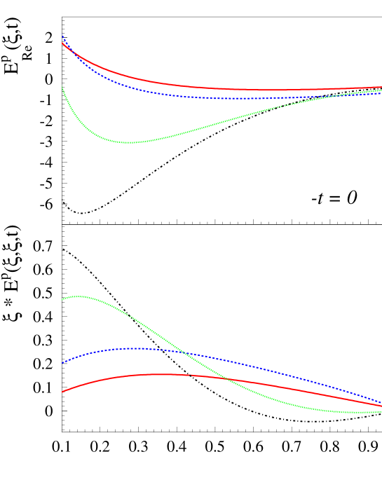
Figure 23: Comparison of the real and imaginary parts of the CFF related with the GPD $E$ for the proton at $t=0$, excluding the $D$-FF subtraction term. The DD parameterization for $J_{u}=0.3$, $J_{d}=0$, and for $b_{val}=b_{sea}=1$ is shown by the solid red curves. The dual parameterization is shown for $J_{u}=0.3$, $J_{d}=0$, and for different values of $\alpha,\beta$ in the model for the forward function $e_{+}$ : $\alpha=0$, $\beta=0$ (dashed-dotted black curves); $\alpha=1$, $\beta=0$ (dotted green curves); $\alpha=2$, $\beta=-0.5$ (dashed blue curves).

4 Data vs Models and Fits

4.1 Comparison of models to current data

In this section, we compare the outputs of the models that we describe in the previous section with the currently existing DVCS data that we presented in section 2.3.

4.1.1 VGG vs data

We begin by exploring a few configurations and options offered by the VGG model. In Fig. 24, we show the JLab Hall A unpolarized (top panel) and beam-polarized (bottom panel) cross sections data [58] as a function of $\phi$. The green dotted curve in the top panel shows the result of the BH calculation. It is at the origin of the characteristic shape of the cross-section which peaks at low and large $\phi$. However, it is clearly not sufficient to fully describe the data. There is certainly room for another process, i.e. DVCS as we believe.

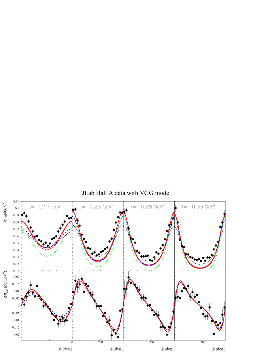
Figure 24: Unpolarized (top row) and beam-polarized (bottom row) cross sections for the $e^{-}p\to e^{-}p\gamma$ reaction. The solid circles are the data points from JLab/Hall A [58]. The dotted green curve is the result of the BH alone calculation. Four different configurations of the VGG model are displayed. The solid red curves are the VGG calculation with only the $H$ GPD, without the D-term, and with $b_{val}=b_{sea}$=1. The dashed red curves are the same but with $b_{val}=b_{sea}$=3. The dotted black curves correspond to this latter calculation with the addition of the $D$-term. The blue dashed curve is the VGG calculation with only the $H$ GPD, without the D-term, and with $b_{val}=b_{sea}$=1 at the slightly shifted kinematics $x_{B}$=0.365 and $Q^{2}$=2.35 GeV² (compared to $x_{B}$=0.36 and $Q^{2}$=2.3 GeV² for the other calculations).

The solid red curve in Fig. 24 shows the result for the BH+DVCS process when only the $H$ GPD, with $b_{val}=b_{sea}$=1 (Eq. (46)) and without the D-term, is included. The calculation is now rather close to the data but nevertheless it doesn’t perfectly describe the $\phi$ distribution. In the $-t=0.17$ GeV² bin, it underestimates the low and large $\phi$ data while it gives a good agreement around $\phi$=180^∘. In the larger $-t$ bins, the situation is opposite: it gives a good agreement with the low and large $\phi$ data while it underestimates the data around $\phi$=180^∘. Regarding the beam-polarized cross sections (bottom panel of Fig. 25), we see that this configuration, with only the $H$ GPD and without the D-term, provides a relatively good agreement with the data for the three lowest $t$-bins. This observable is therefore largely dominated by the $H$ GPD, which was expected (see Eq. (31)). One notes however a disagreement between the data and the calculation for the largest $t$-bin. This might be a shortcoming of the VGG model in the $H$ parameterization but this might also be a sign of higher-twist effects turning in as $-t$ increases, as these calculations, we recall, have been done at the leading-twist order.

The dashed red curve in Fig. 24 shows the result of the same configuration but for $b_{val}=b_{sea}$=3. The effect is to decrease the unpolarized cross section by several percents at low $-t$ and the beam-polarized cross section by a couple of percent (in absolute value) for all $-t$ values. The effect of these parameters is therefore not dramatic.

The black dotted curves in Fig. 24 show the inclusion of the $D$-term in the previous calculation. We recall that the D-term contributes to both $H$ and $E$ GPDs, so that this calculation contains also an $E$ contribution. The $D$-term has a significant influence on the cross section: it tends to increase the cross section around $\phi$=180^∘ and thus improve the agreement with the data but at the same time it reduces the cross section at low and large $\phi$ which is actually not particularly desired. The inclusion of the $D$-term in the calculation has no effect on the beam-polarized cross section (the dashed blue and black dotted curves are superposed in Fig. 24-bottom panel). Indeed, this observable is sensitive only to the imaginary part of the DVCS amplitude (see Eq. (31)) while the $D$-term, which lives uniquely in the $-\xi\leq x\leq\xi$ region, contributes only to the real part.

Finally, we wanted to highlight the importance of determining precisely the kinematics of the observables, an issue that we brought up in section 2.2. The values of $x_{B}$ and $Q^{2}$ provided by Ref. [58] are respectively 0.36 and 2.3 GeV². Since this leaves free the third digit, we explore the kinematics corresponding to $x_{B}$=0.365 and $Q^{2}$=2.35 GeV², i.e. a set of extreme values yielding the rounding $x_{B}$=0.36 and $Q^{2}$=2.3 GeV². The dashed blue curve in Fig. 24 show the result, for the configuration with only the $H$ GPD contribution with $b_{val}=b_{sea}$=1 and without the $D$-term (i.e. directly comparable to the solid red curves). The effect is non-negligible, decreasing the unpolarized cross section by up to 15% at the lowest $-t$ values and the beam-polarized cross sections by even a larger amount. Keeping this potential effect in mind, we continue our studies in the following with the published $x_{B}$=0.36 and $Q^{2}$=2.3 GeV² kinematics.

We do not display calculations with the $\tilde{E}$ GPD because its only effect on the observables of Fig. 24 is to increase by 1 or 2% the unpolarized cross section (it cannot contribute to the beam-polarized cross section).

Having discussed these few effects on the $H$ GPD, we are now going to focus on the effect of the $\tilde{H}$ and $E$ GPDs. In the following figures, we will keep $b_{val}=b_{sea}$=1 for $H$. We will compare the VGG calculations to the JLab Hall A, CLAS and HERMES data. We will show systematically four sets of curves and configurations:

• Only the GPDs $H$ contribution, without the $D$-term. In the following figures, this configuration will be described by the red solid curves.

• Adding, with respect to the previous configuration, the $\tilde{H}$ contribution. This configuration will be described by the dashed red curves.

• Adding, with respect to the previous configuration, the $E$ GPD with its valence and sea contributions (see Eq. (57)). The values of ($J_{u}$, $J_{d}$) are taken as (0.3, 0.). The D-term contribution to $H$ and $E$ is included. In the figures, this configuration will be described by the black dash-dotted curves.

• Changing, with respect to the previous configuration, the values of ($J_{u}$, $J_{d}$) which are taken as (0., 0.3). In the figures, this configuration will be described by the blue dashed curves.

Fig. 25 shows the results of these four calculations for the JLab Hall A unpolarized and beam-polarized cross sections. By comparing the dashed red curves ($\tilde{H}$+$H$ contribution) to the solid red curves ($H$-only calculation), one sees that the $\tilde{H}$ GPD has very little effect on the unpolarized cross section as the two curves are barely distinguishable in the top panel of Fig. 24. The effect of $\tilde{H}$ on the beam-polarized cross section is more visible. It tends to increase by $\approx$ 15% the amplitude of the sine-like modulation.

One sees that the VGG $E$ GPD has almost no influence on the beam polarized cross section as the black dash-dotted curves and the blue dashed curves are essentially superposed on the dashed red curves in Fig. 25-bottom panel. The beam polarized cross section is thus largely dominated by $H$ with a small extra contribution of $\tilde{H}$. Concerning the unpolarized cross section, the sizable influence of the GPD $E$ is essentially through the $D$-term as the dashed-dotted black curves and dashed blue curves of Fig. 25-top panel are almost indistinguishable. In other words, there is no sensitivity of the unpolarized cross section to the ($J_{u}$, $J_{d}$) contribution of the $E$ GPD.

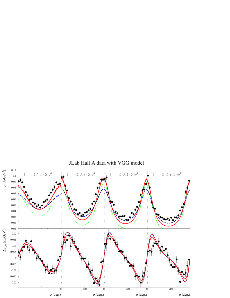
Figure 25: Unpolarized (top row) and beam-polarized (bottom row) cross sections for the $e^{-}p\to e^{-}p\gamma$ reaction. The solid circles are the data points from JLab/Hall A [58]. Four different configurations of the VGG model are displayed. The solid red curves are the VGG calculation with only $H$. The dashed red curves are the same calculation with the addition of the $\tilde{H}$ contribution. The dashed-dotted black curves are the same with the addition of the $E$ GPD with its valence and sea contributions with ($J_{u}$,$J_{d}$)=(0.3,0.) and the $D$-term. The dashed blue curves are the same but with ($J_{u}$,$J_{d}$)=(0.,0.3). The dotted green curve is the result of the BH alone calculation.

In Fig. 26, we compare the four VGG calculations to the beam spin asymmetries of the CLAS collaboration. We recall that these asymmetries are the ratio of the beam-polarized to the unpolarized cross sections. Since the VGG calculation with only $H$ and with or without $\tilde{H}$ is in general underestimating the unpolarized cross section while describing correctly the beam-polarized cross section at low $-t$, as we saw in Fig. 25, it should be expected that the beam spin asymmetry be overestimated at low $-t$. This is indeed what we observe in Fig. 26. Since the addition of $\tilde{H}$ increases the amplitude of the beam polarized cross section (Fig. 25-bottom panel), the corresponding asymmetry is also amplified. At larger $-t$ ($>\approx$ 0.8 GeV²), where the leading-twist handbag formalism is expected to be less valid, the agreement between the data and the calculation is better. However, we saw in Fig. 25 that, for the largest $-t$ bin, the VGG calculation was overestimating the beam-polarized cross section so that the better agreement for the beam spin asymmetry might simply result of the ratio of two overestimated quantities. This clearly shows the limit of comparing calculations to one single asymmetry.

Adding $E$ in the VGG calculation (black dash-dotted and blue dashed curves in Fig. 26) moves the VGG beam-spin asymmetries calculations closer to the data. This could be expected since the addition of $E$ tends to increase the cross section around $\phi$=90^∘ (see Fig. 25). However, some discrepancy clearly remains. One can also note that in general, as $Q^{2}$ increases, the agreement between the calculations and the data tends to improve.

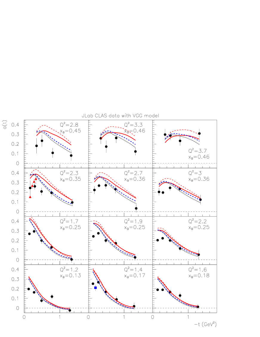
Figure 26: Beam spin asymmetries at $\phi$=90^∘ as a function of $t$ as measured by the CLAS collaboration [61] with VGG calculations. The convention for the curves is the same as in Fig. 25.

We finally compare in Fig. 27 our four VGG calculations to the lower $x_{B}$ HERMES domain. We show in this figure the nine asymmetry $\phi$ moments which are expected to be non-null in the leading-twist handbag formalism. We added as a tenth observable the $A_{UL}^{\sin 2\phi}$ moment (bottom right plot in Fig. 27) which is expected to be small (suppressed by powers of $Q$) in this approximation. However the data shows a rather large asymmetry which cannot be described by any leading-twist handbag calculation, whatever the parameterization of the GPDs.

In Fig. 27, we see that the main trends of the data are reproduced by the VGG model: for instance, as $-t$ increases, the trend towards increasing negative values of $A_{C}$ and $A_{Uy,I}^{\cos\phi}$, the rise of $A_{C}^{\cos\phi}$ and $A_{Uy,I}$, etc… Except for the amplitudes of $A_{C}$ and $A_{C}^{\cos\phi}$ which are overestimated, the VGG calculation provides a good description of the amplitudes of the nine leading-twist observables. We note the particular sensitivity of $A_{C}$ and $A_{C}^{\cos\phi}$ to the $E$ GPD. It actually mostly comes from the $D$-term contribution to $E$, since there is little difference between the dashed-dotted black and dashed blue curves (non-$D$-term contribution to $E$). However, since $A_{C}$ and $A_{C}^{\cos\phi}$ are largely overestimated, it seems that no really reliable conclusion on $E$ or the $D$-term can be extracted at the moment.

The transversally polarized target asymmetries are also expected to be particularly sensitive to $E$ and one does see some difference between the two ($J_{u}$, $J_{d}$) configurations. However, we see that these observables are actually largely dominated by $H$ and that $E$ comes only as a small variation around $H$. It is also difficult in those conditions to extract a reliable information on $E$, as long as $H$ is not determined a the few percent accuracy.

As expected, $A_{UL}^{\sin\phi}$ is particularly sensitive to the $\tilde{H}$ GPD contribution, which is necessary in order to explain the magnitude of the data. Finally, the large amplitude of the $A_{UL}^{\sin 2\phi}$ moment is a puzzle.

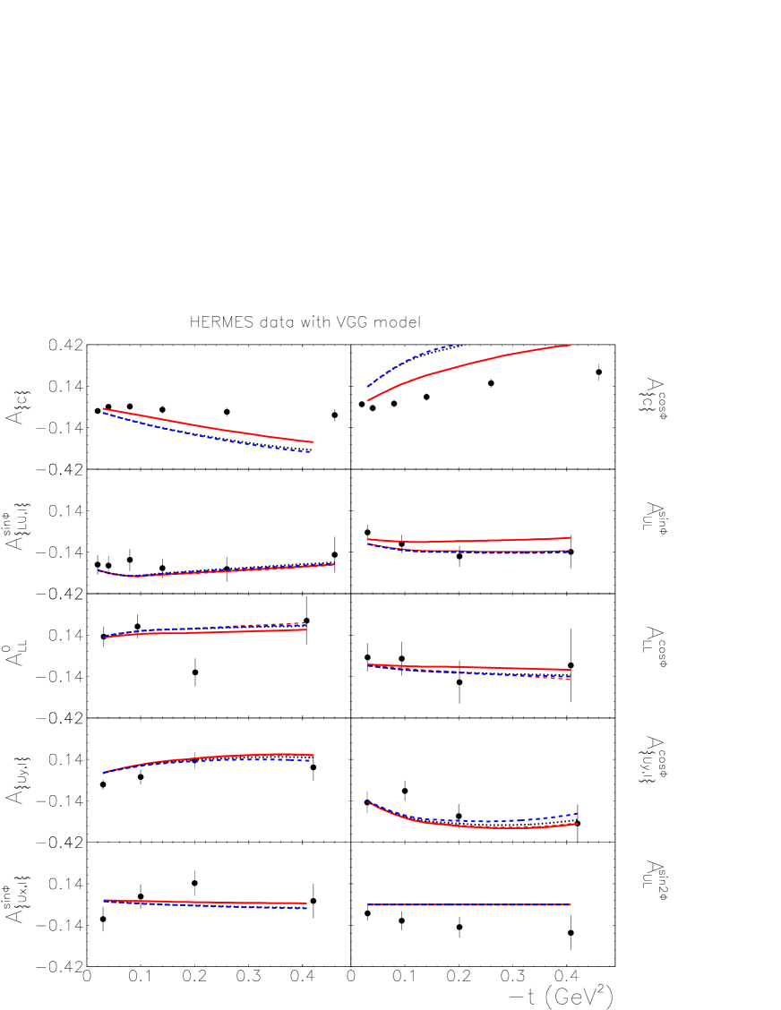
Figure 27: Ten azimuthal moments as a function of $-t$ as measured by the HERMES collaboration [64, 65, 66, 67, 68, 69, 70, 71] with VGG calculations. The convention for the curves is the same as in Fig. 25.

4.1.2 The GK model vs data

We have ran the GK model in three different configurations:

• Keeping only the GPD $H$. In the figures, this configuration will be described by the red solid curves.

• Adding with respect to the previous configuration the contribution of the $\tilde{H}$ GPD. This configuration will be described by the dashed red curves

• The “full model”, i.e. with the contributions of all four GPDs. This configuration will be described by the black dash-dotted curves.

Fig. 28 shows the results of these three calculations for the unpolarized and beam-polarized cross sections as measured by the JLab Hall A data [58].

We observe some features very similar to the VGG calculation. The beam-polarized cross section (bottom panel of Fig. 28) is well described for the three lowest $-t$ bins and is mostly the result of the $H$ GPD contribution. The inclusion in the calculation of the $\tilde{H}$ GPD increases, like for VGG and in about the same proportions, the amplitude of the polarized cross section. Since the dashed-dotted black curves (“full model”) are essentially superposed on the dashed red curves, we conclude that $E$ (and $\tilde{E}$) have basically no influence on this observable. In the largest $-t$ bin, the GK calculation tends to overestimate the data although to a lesser extent than VGG.

For the unpolarized cross section (top panel of Fig. 28), we also see features similar to the VGG model. The calculation with only the $H$ GPD is rather close to the data but is not fully satisfactory. There is clearly some missing strength for $\phi$ around 180^∘, where the handbag DVCS contribution is expected to be dominant. Adding the contribution of the other GPDs barely makes a difference. It might even slightly decrease the cross section around $\phi$=180^∘, worsening the situation. We recall that the GK model has no $D$-term implemented.

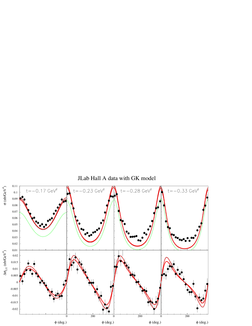
Figure 28: Unpolarized (top row) and beam-polarized (bottom row) cross sections for the $e^{-}p\to e^{-}p\gamma$ reaction. The solid circles are the data points from JLab/Hall A [58]. Three different configurations of the GK model are displayed. The solid red curves are the GK calculation with only the $H$ GPD. The dashed red curves are the GK calculation with in addition the $\tilde{H}$ GPD. The dashed-dotted black curves are the “full” GK calculation, i.e. with the contribution of all GPDs. The dotted green curve is the result of the BH alone calculation.

Fig. 29 compares the CLAS beam spin asymmetries with the GK calculations. As could be anticipated, the beam spin asymmetries are in general overestimated at low $-t$ since the unpolarized cross sections are underestimated (top panel of Fig. 29) and the beam-polarized cross sections are correctly reproduced (bottom panel of Fig. 29). Adding the contribution of the GPDs other than $H$ tends to increase the disagreement between the calculation and the data. This can be attributed to the decrease of the unpolarized cross section that we noted in Fig. 28-top panel. However, like for VGG, we observe that the GK calculation provides a better agreement with the data for the largest $Q^{2}$ values, in which case, the inclusion of the GPDs other than $H$ does help.

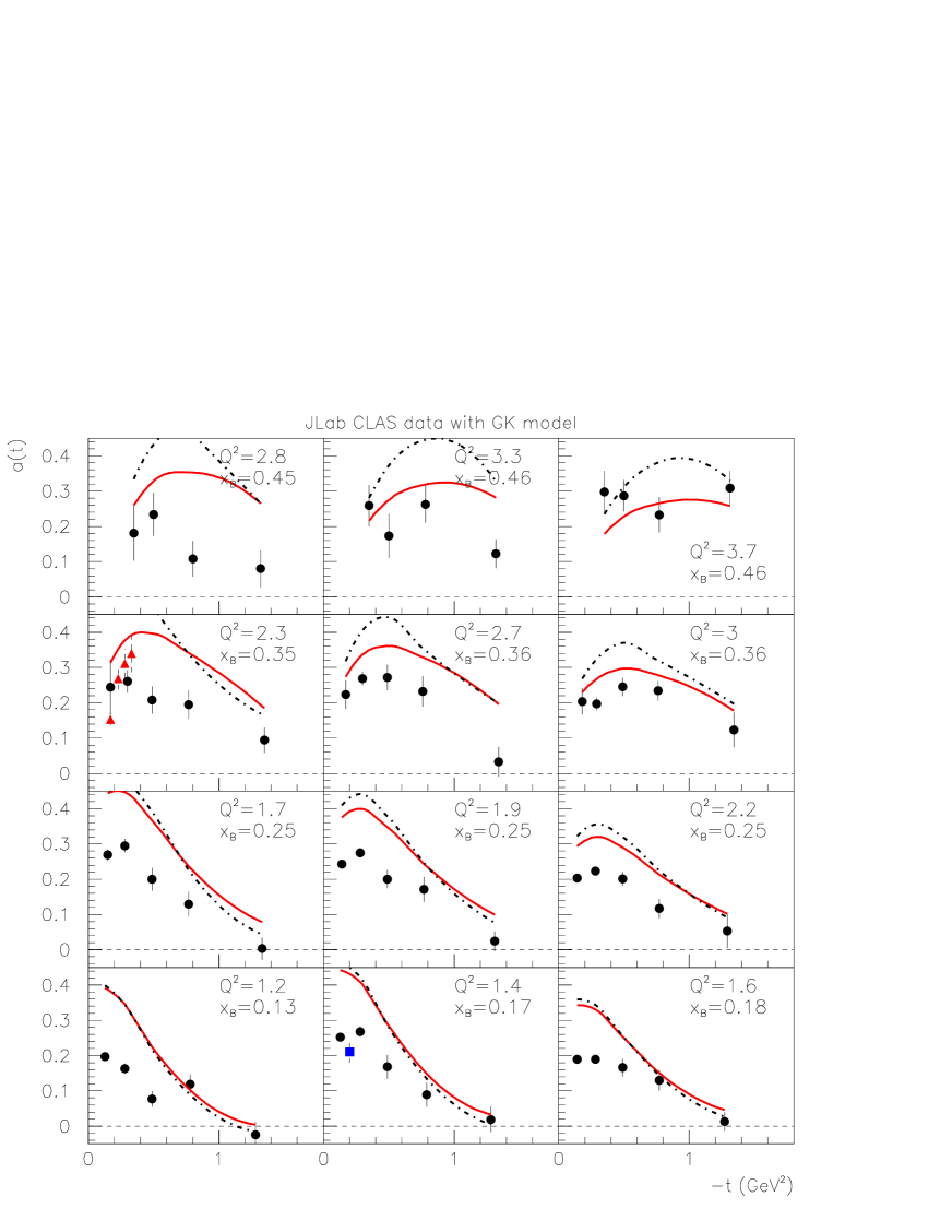
Figure 29: Beam spin asymmetries at $\phi$=90^∘ as a function of $t$ as measured by the CLAS collaboration [61] with GK calculations. The convention for the curves is the same as in Fig. 28.

Fig. 30 compares the HERMES azimuthal moments with the GK calculation. Like for VGG, the general trend of the data is correctly reproduced. A notable difference is that the amplitudes of the $A_{C}$ and $A_{C}^{\cos\phi}$ moments agree much better with the data. This can in part be attributed to the absence of a $D$-term in the GK calculation as we saw that; in the VGG model, it was a major contribution, both to $H$ and $E$. We notice again that the$A_{Uy,I}$ moments are largely dominated by the contribution of the $H$ GPD and that any reliable extraction of the comparatively small $E$ contribution requires a control of $H$ at the few percent level. Like in VGG, the strong $A_{UL}^{\sin 2\phi}$ moment is a mystery.

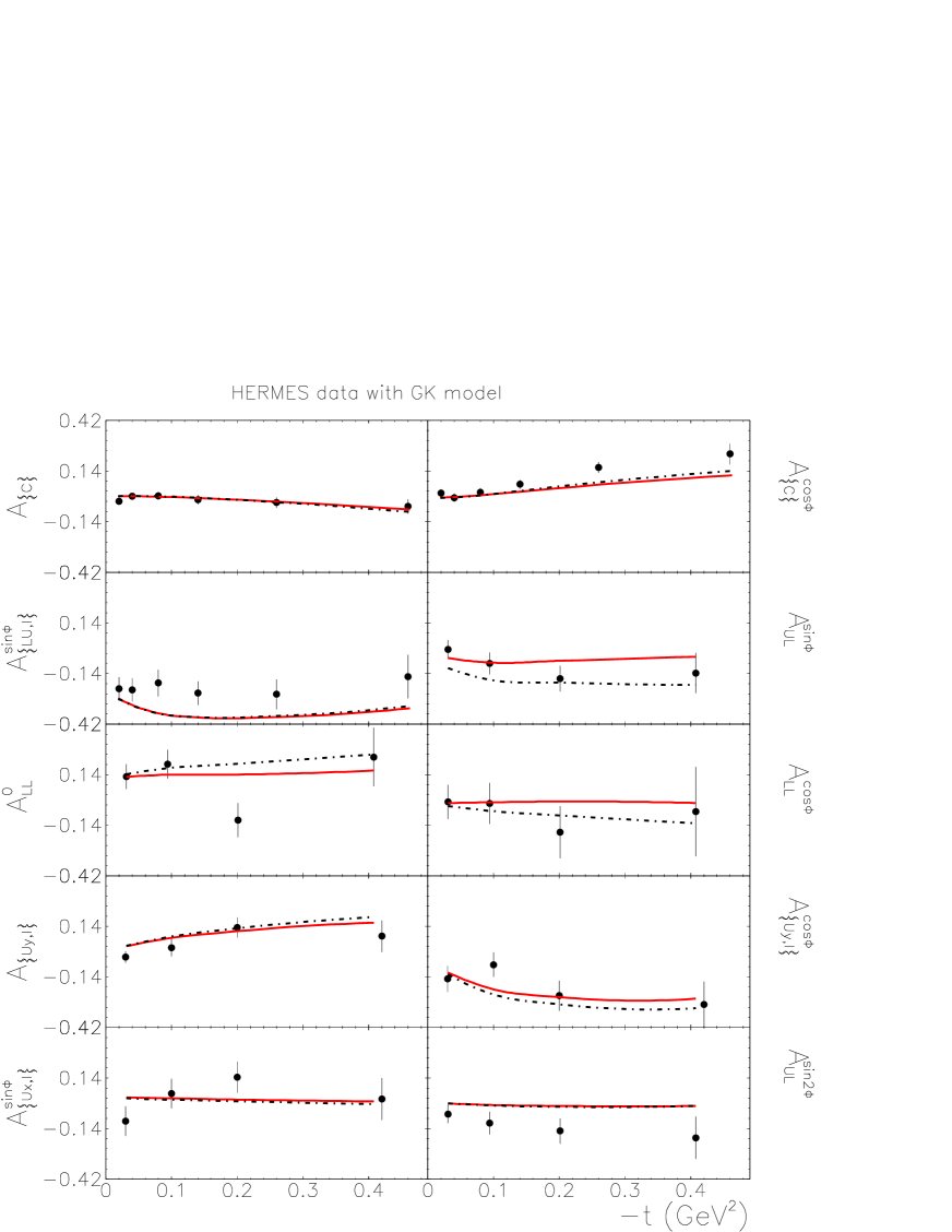
Figure 30: Ten azimuthal moments as a function of $-t$ as measured by the HERMES collaboration [64, 65, 66, 67, 68, 69, 70, 71] with GK calculations. The convention for the curves is the same as in Fig. 28.

4.1.3 The dual model vs data

We have ran the dual model in three different configurations:

• Keeping only the GPDs $H$, without D-term, i.e. for $d_{1}=0$. In the figures, this configuration will be described by the red solid curves.

• Adding, with respect to the previous configuration, the $E$ GPD with $d_{1}=-4/3$ and ($J_{u},J_{d}$)= (0.3, 0.). The ($\alpha,\beta$) values in the model for the function $e^{+}(x,t)$ (Eq. (103)) are taken as (0., 0.). In the figures, this configuration will be described by the black dash-dotted curves.

• Changing, with respect to the previous configuration, the values of ($\alpha,\beta$) (Eq. (103)) to (2., -0.5). In the figures, this configuration will be described by the blue dashed curves.

Fig. 31 shows the results of these three calculations for the unpolarized and beam-polarized cross sections as measured by the JLab Hall A data [58].

The beam-polarized cross sections (bottom panel of Fig. 31), are very well described for the three lowest $-t$ bins. This gives support to the description of the $H_{Im}$ CFF in the dual model. One can note that there is a little influence (a few percents) of the $E$ GPD on this observable. Like for the previous models (VGG and GK), the largest $-t$ bin shows a discrepancy between the calculation and the data.

Regarding the unpolarized cross section (Fig. 31-top), we see that having only the GPD $H$ for the DVCS contribution is not sufficient to describe the data. We note that the GPD $H$ in the dual model brings less strength to the unpolarized cross section than in the VGG and GK models (see Figs. 25 and 28). Like for the VGG and GK models, adding a $E$ GPD contribution doesn’t improve the situation: it increases the cross section around $\phi$=180^∘ but decreases it at low and large $\phi$.

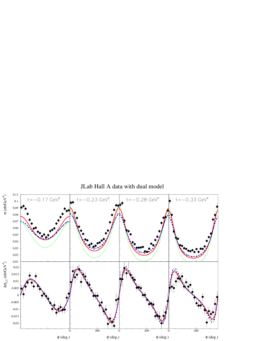
Figure 31: Unpolarized (top row) and beam-polarized (bottom row) cross sections for the $e^{-}p\to e^{-}p\gamma$ reaction. The solid circles are the data points from JLab/Hall A [58]. Three different configurations of the dual model are displayed. The solid red curves are the dual parameterization for the vector amplitude (GPD $H$) only (without D-term, i.e. for $d_{1}=0$). The other curves are the dual parameterization including both GPD’s $H$ and $E$, for $d_{1}=-4/3$, $J_{u}=0.3$, $J_{d}$ = 0, and for different values of $\alpha,\beta$ in the model for the function $e_{+}(x,t)$ : $\alpha=0$, $\beta=0$ (dashed-dotted black curves), and $\alpha=2$, $\beta=-0.5$ (dashed blue curves). The dotted green curve is the result of the BH alone calculation.

In Fig. 32, we compare the three dual calculations to the beam spin asymmetries of the CLAS collaboration. We observe the same features as with the VGG and GK calculations, i.e. the best agreement between the data and the calculation for the couple of bins with $Q^{2}>$ 3 GeV² bins but otherwise an overestimation (by 20 to 30%) of the data. This is obviously due to the underestimation of the unpolarized cross section. Adding a contribution of the $E$ GPD can bring the calculation a bit closer (or further) to the data according to the parameterization chosen but this is clearly not a main factor.

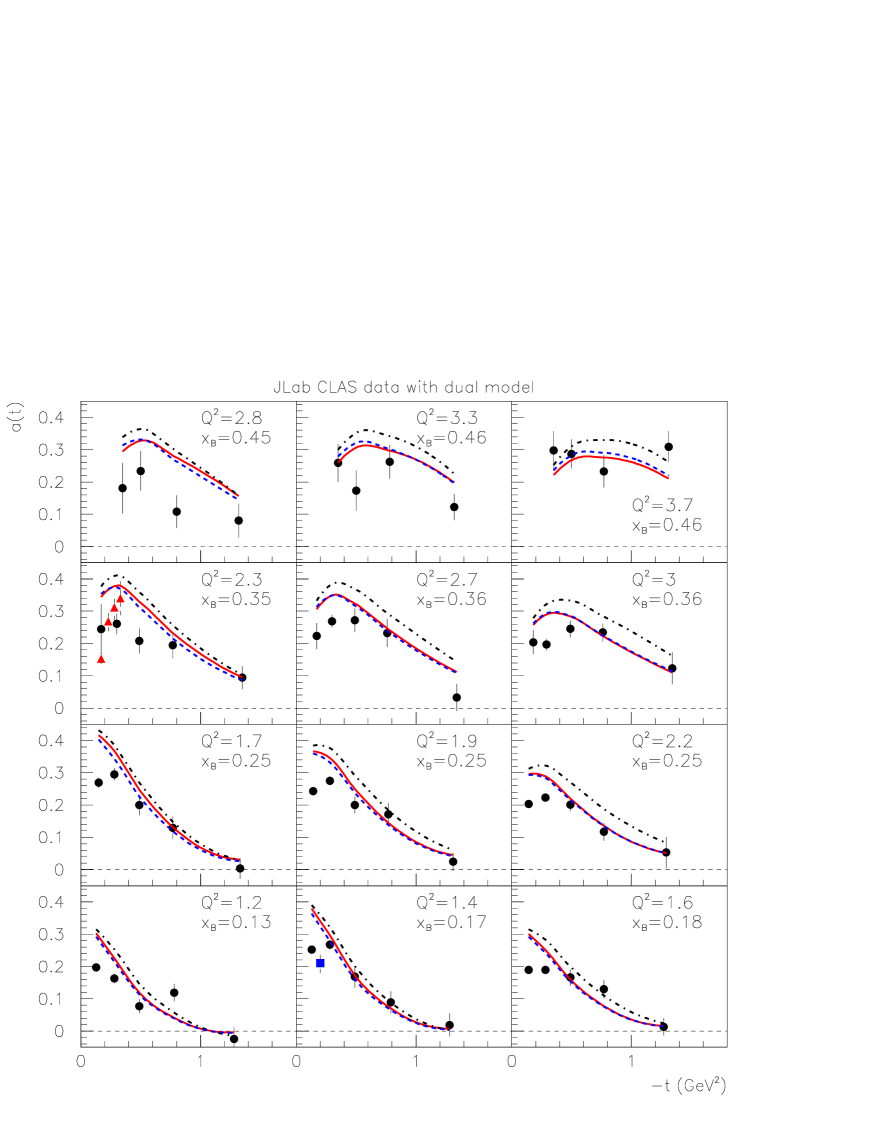
Figure 32: Beam spin asymmetries at $\phi$=90^∘ as a function of $t$ as measured by the CLAS collaboration [61] with the dual model calculations. The convention for the curves is the same as in Fig. 31.

In Fig. 33, we compare the three dual calculations to the azimuthal moments measured by the HERMES collaboration. We observe the same trends as for the VGG and GK models, i.e. a general good description of the trend of the data. However, in the details, the $A_{C}$ and $A_{C}^{\cos\phi}$ amplitudes are overestimated. The strong sensitivity of the $A_{Uy,I}^{\cos\phi}$ moment of the $E$ GPD is again noticed. Here, the data clearly favor the $\alpha=2$, $\beta=-0.5$ configuration for the parameterization of the $e^{+}(x,t)$ function.

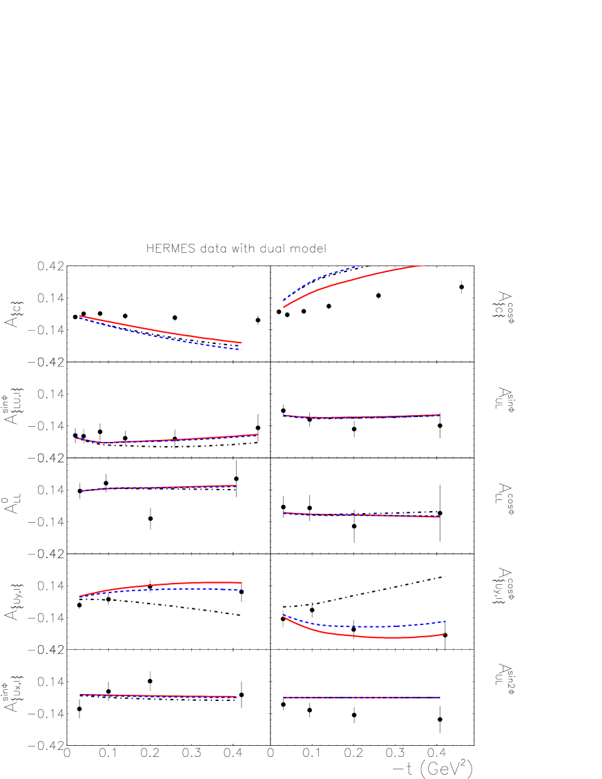
Figure 33: Ten azimuthal moments as a function of $-t$ as measured by the HERMES collaboration [64, 65, 66, 67, 68, 69, 70, 71] with the dual model calculations. The convention for the curves is the same as in Fig. 31.

4.1.4 The KM model vs data

The KM model is the model originally developped by K. Kumericki and D. Mueller [113] based on the Mellin-Barnes parameterization of GPDs which we discussed in section 3.3. The parameters of the KM model are determined from fitting H1/ZEUS, HERMES (with or without target polarization data) and JLab data (CLAS and with or without Hall A). In the following, we have used three versions of the code:

• KM10: in this version, the four GPDs are considered: $H$ and $\tilde{H}$ are modeled for their valence part by Eq.( 120), the $E$ contribution is only through the D-term and $\tilde{E}$ by the pion pole (like in VGG and GK). There are fifteen free parameters. They are $b$ (val), $r$ (val) and $M$ (val) for the valence part of $H$ (see Eq.( 120)), three similar ones $\tilde{b}$ (val), $\tilde{r}$ (val) and $\tilde{M}$ (val) for the valence part of $\tilde{H}$, $C$ and $M_{C}$ for the D-term (see Eq.( 121)), two for the pion pole (one for the normalization and one for the $t$-dependence) and five for the small $x$ behavior of $H$: $M$ (sea) which controls the $t$-dependence trough a dipole ansatz, $s_{2}$ (sea), $s_{2}$ (gluon) , $s_{4}$ (sea) and $s_{4}$ (gluon) which control the normalization and evolution flow of the sea and gluon contributions. One should however note that the five latter parameters are determined by the collider experiments which are then just propagated to the valence region. In other words, the JLab and HERMES data that we discuss in this review only impact the first ten parameters and the KM10 model can effectively be considered as having 10 free parameters in this framework. These parameters are determined by fitting the JLab Hall A, CLAS beam spin asymmetries and HERMES data, excluding the polarized target data. The values of the free parameters and more details in the ingredients of the model are given explicitely in Ref. [111]. In the following figures, this version will be described by the black dot-dashed curves.

• KM10a: compared to the KM10 version, this version sets $\tilde{H}$ to zero and fixes the pion pole, which removes five free parameters and therefore reduces the total number of free parameters to five. These are determined by fitting only the HERMES (without the polarized target data) and CLAS data, i.e. excluding the JLab Hall A data of the fit. The JLab Hall A cross sections are indeed notoriously difficult to describe, as was illustrated by the comparison of the VGG, GK and dual models with data shown in the previous sections. We will see shortly that this “minimal” version of the KM model is indeed unable to describe or predict the JLab Hall A cross sections. In the figures, this version will be described by the red solid curves.

• KMM12: this latest version of the KM model includes the HERMES polarized target data in the fit (as well as the JLab Hall A data) and has the same ten free parameters than KM10. The values of these parameters and the detailed ingredients of this version of the model are given in Ref. [112]. In the figures, this version will be described by the blue dashed curves.

We mention that the code for the KM10 and KM10a versions of the model can be found on the public link of Ref. [110]. We are thankful to K. Kumericki and D. Mueller for having provided us with a private version of the KMM12 code.

The results of the three KM model versions are displayed in Fig. 34 in comparison to the JLab Hall A unpolarized (top panel) and beam-polarized (bottom panel) cross sections data. The solid red curves (KM10a model), which don’t include the JLab Hall A data in the determination of the parameters are essentially the result of the $H$ contribution (with some $E$ contribution through the D-term and $\tilde{E}$ contribution through the pion pole, as discussed earlier). We then find results similar to those obtained with the three previous models that we discussed, i.e. that the unpolarized cross sections are underestimated while the beam-polarized cross section are approximatively well described. It is only with the addition of a $\tilde{H}$ contribution (KM10 or KMM12 models) that an agreement is obtained for the description of the unpolarized cross section. An issue is that this $\tilde{H}$ contribution is about a factor 3 larger than values given by standard parameterizations, such as in VGG or GK. In the KM model, $\tilde{H}$ could therefore be viewed as an effective GPD contribution, not clearly linked to polarized PDFs. The inclusion of the HERMES polarized target data in the fit (blue dashed curve) does not strongly affect the description of the Hall A data (one essentially notes a change of $\approx$ 10% for the unpolarized cross section lowest $\mid t\mid$ bin).

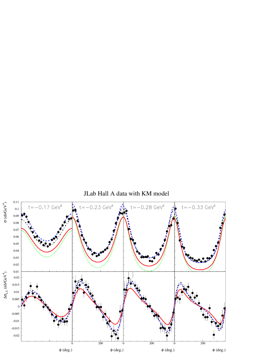
Figure 34: Unpolarized (top row) and beam-polarized (bottom row) cross sections for the $e^{-}p\to e^{-}p\gamma$ reaction. The dotted green curve is the result of the BH alone calculation. The solid circles are the data points from JLab/Hall A [58]. Three different versions of the KM code are displayed. The red solid curves are the results of the 5-free parameter model version with the Hall A data and the HERMES polarized target data excluded from the fit (version KM10a). The black dot-dashed curves are the results of the 10-free parameter model version with the Hall A data included in the fit, but not the HERMES polarized target data (version KM10). The blue dashed curves are the results of the 10-free parameter model version with the HERMES polarized target data included in the fit (version KMM12).

In Fig. 35, we compare the results of the KM model versions to the CLAS beam spin asymmetries. The comparison between the data and the calculations is available only on some limited range, i.e. $Q^{2}>$ 1.5 GeV² and $-t<<Q^{2}$, due to the restrictions in the KM code. We note that those are actually very reasonable limits for the application of the GPD formalism in DVCS and should probably be valid for all models, not only KM. All three versions of the KM model describe relatively well the data which is expected since these data are included in the fit of the parameters for all three configurations. The behavior of the three model versions differ somewhat but the data do not allow to favor one more than the others.

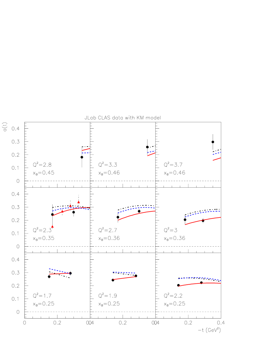
Figure 35: Beam spin asymmetries at $\phi$=90^∘ as a function of $t$ as measured by the CLAS collaboration [61] with the KM model calculations. The convention for the curves is the same as in Fig. 34.

In Fig. 36, we finally compare the results of the KM model versions to the HERMES azimuthal moments. The polarized target data are described only by the KMM12 version of the code, which explicitely took those data in the fit. It achieves a relatively good description of the nine leading-twist asymmetry moments. As usual, the $A_{LU}^{\sin 2\phi}$ is not explained but since it is not related to the DVCS leading-twist formalism, this should not come as a surprise.

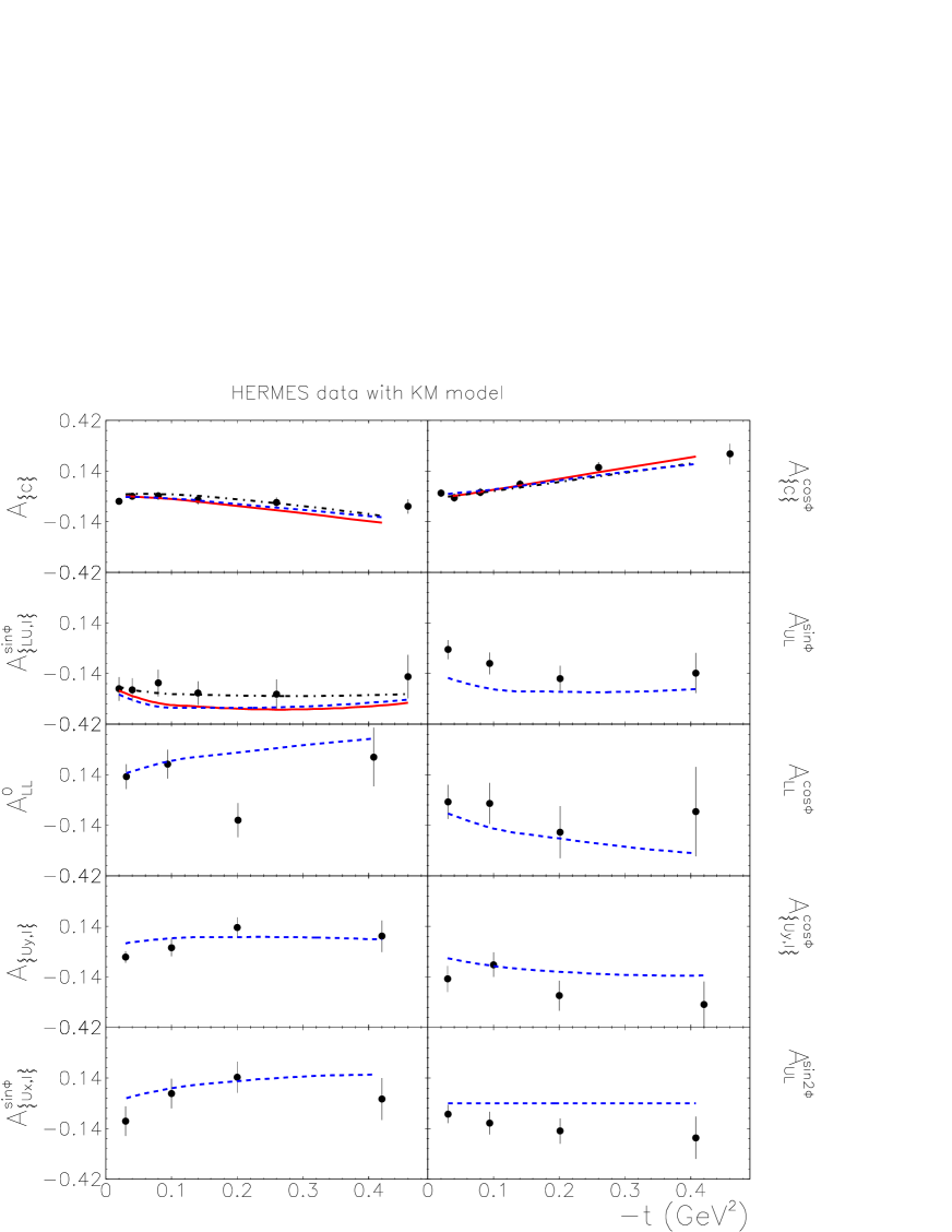
Figure 36: Ten azimuthal moments as a function of $-t$ as measured by the HERMES collaboration with the KM model calculations. The convention for the curves is the same as in Fig. 34.

In summary, the KM model, in particular the KMM12 version, is, to this day, the only model available on the market which achieves a relatively good description (with an overall normalized $\chi^{2}$ of $\approx$ 1.55 for 95 data points [112]) of all presently available DVCS data in the valence region (and even beyond, at lower $x_{B}$ values). The challenge lied particularly in the description of the JLab Hall A data, for which the other three models that we discussed failed to give a satisfying description. Though, the price to pay has been to introduce in KM a strong $\tilde{H}$ contribution, which remains to be understood.

4.2 CFF fits

In the previous section, we have compared the JLab Hall A, CLAS and HERMES DVCS data with four models with adjustable parameters: VGG, GK, the dual model and KM. Although many general trends of the data are reproduced by these four models, none can claim to have a perfect global description of all data with fully reliable inputs (in particular, the meaning of the strong $\tilde{H}$ contribution in KM, which achieves the best $\chi^{2}$ fit all the data sets, remains to be understood). Specifically, the observable which is the most challenging to reproduce is the JLab Hall A unpolarized cross section. The question arises if this deficiency is due to the limitations of the models which imposes some particular functional form for the ($x,\xi,t$)-dependence of the GPDs that might be too constraining or if the data simply don’t lend themselves in general to a leading-twist and leading-order handbag formalism.

To give some element of response to this question, we now present an alternative way to work on the data. Instead of starting from a model whose parameters, in the frame of a particular functional form, are to be fitted to the data, another approach is to directly take the CFFs as free parameters and fit them to the data for each individual kinematic point. As we saw with (see Eqs.( 31-34) for a few examples), there are well established relations (at least at the leading-twist and leading order) between the CFFs and the observables and they depend only on kinematical factors. At a given ($E_{e},x_{B},Q^{2},t,\phi$) experimental point, these kinematical factors can be determined and the idea is thus, for each ($E_{e},x_{B},Q^{2},t,\phi$) experimental point, to fit simultaneously the various observables available for this particular kinematics, taking the CFFs as free parameters. The main advantage of this approach is to be model-independent (in the limit that the leading-twist and leading order relation between the observables and the CFFs are valid), as the CFFs can vary freely without being constrained or restrained by a particular function. The main shortcoming of this approach is that CFFs are fitted, i.e. not GPDs themselves. We recall that CFFs, which depend only on $\xi$ and $t$ while GPDs depend on $x$, $\xi$ and $t$, are (weighted) integrals of the GPDs (over $x$) or GPDs at the lines $x=\pm\xi$. Therefore, in order to access GPDs, there is, in a second stage, an unavoidable additional model-dependent deconvolution to carry out. Nevertheless, we will see in the following that already extracting CFFs, in a model-independent way as much as possible, as a first step towards GPDs, carries a lot of interest.

We describe in the following the work in this direction of Refs. [126, 127, 128, 129, 125, 112].

4.2.1 “Brute force” least square minimization

The method was pioneered in 2008 in Ref. [126]. Knowing the well-established BH and DVCS amplitudes (see Eq.(17) for the latter process), which provides the relation between the observables and the CFFs, the procedure consists in fitting, at each ($x_{B}$, $Q^{2}$, $-t$) kinematic point, the $\phi$ distribution (or the moment) of all the available observables at this kinematic point, taking the eight CFFs as free parameters. In Refs. [126, 127, 128, 129], actually only seven CFFs were considered: $H_{Re}$, $E_{Re}$, $\tilde{H}_{Re}$, $\tilde{E}_{Re}$, $H_{Im}$, $E_{Im}$ and $\tilde{H}_{Im}$. In this work, the eighth CFF $\tilde{E}_{Im}$ has been set to 0. The reason is that, as was seen in section 3, it is common to model the $\tilde{E}$ GPD by the pion pole, which contributes only to the real part of the DVCS amplitude. This is essentially the only model assumption in this procedure. Otherwise, the other CFFs are free to vary within a 7-dimensional hypervolume, which is only bounded by conservative limits: $\pm$5 times the values of the VGG CFFs. We recall that some GPDs have to satisfy a certain number of normalization constraints. These are all fulfilled by the VGG model and it should be clear that $\pm$5 times the VGG CFFs make up conservative bounds.

It is clear that fitting only one observable with seven free parameters does not converge. All data can be fitted with high quality but many combinations of the seven CFFs provide an equally good fit and no information can really be extracted on any CFFs. However, it was striking to observe in Ref. [126] that fitting simultaneously two observables, namely the unpolarized and the beam-polarized cross sections of Hall A, with the seven CFFs as free parameters, resulted in a convergence for two CFFs, i.e. $H_{Re}$ and $H_{Im}$. This resulted for the first time in quasi-model-independent constraints on the $H_{Re}$ and $H_{Im}$ CFFs for the Hall A kinematics. Fig. 37 shows the resulting fits of the Hall A data and Fig. 38-left column the resulting $H_{Re}$ and $H_{Im}$ CFFs obtained, displayed as a function of $-t$.

The reason for the convergence of the particular $H_{Re}$ and $H_{Im}$ CFFs is, as we saw in section 4.1, that the unpolarized and the beam-polarized cross sections are largely dominated by these two CFFs (respectively). The fitting procedure allows to determine central values for these two CFFs which are the values which minimize the $\chi^{2}$ between the theory and the data, and two error bars, which correspond to $\chi^{2}+1$. These error bars are asymmetric which reflects the non-linearity and undersconstrained nature of the problem (we recall that CFFs enter as bilinear combinations in a cross section). The error bars that are obtained reflect actually not the statistical accuracy of the data (which are precise at the few percent level) but the influence of the five other CFFs which are subdominant and do not converge to a particularly well defined value within the 7-dimensional hypervolume defined previously. The error bars are therefore correlation error bars. If, guided by some theoretical considerations, one can reduce the number of CFFs entering the fit as free parameters (like it is done for $\tilde{E}_{Im}$ or like it will be done in the next section by keeping only the $H$ GPD) or if one can reduce their range of variation into an hyperspace smaller than $\pm$ 5 times the VGG CFFs as has been done here, the error bars can obviously only diminish. In this case, one has clearly to make sure that the assumptions are well founded, otherwise, errors will of course be underestimated. The present approach should be considered as a most conservative estimation of uncertainties and as minimally theory-biased.

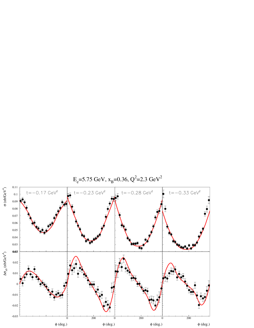
Figure 37: Result of the fit of the unpolarized (top panel) and beam-polarized (bottom panel) cross sections of the $e^{-}p\to e^{-}p\gamma$ reaction by the fitter code of Ref. [126] leaving seven CFFs free.

In these conditions, with this fitting algorithm, it was possible to determine :

• as we just discussed, the $H_{Im}$ and $H_{Re}$ CFFs at $<x_{B}>\approx 0.36$, and for three $t$ values, by fitting simultaneously [126] the JLab Hall A proton DVCS beam-polarized and unpolarized cross sections [58] (see Fig. 38-left column). For the lowest $-t$ values, the fitting procedure could not identify a central value for $H_{Re}$ with well-defined error bars and so we display only $H_{Im}$. One should also notice that the fit of the largest $-t$-bin is not perfect ($\chi^{2}\approx$ 3) as can be seen in Fig. 37. Therefore, the small error bar obtained for $H_{Re}$ at $-t=$0.33 GeV² might be underestimated, the meaning of an error bar on a fitting parameter for a bad $\chi^{2}$ fit being not straightforwardly interpretable.

• the $H_{Im}$ and $\tilde{H}_{Im}$ CFFs, at $<x_{B}>\approx 0.35$ and $<x_{B}>\approx 0.25$, and for three $t$ values, by fitting simultaneously [128] the JLab CLAS proton DVCS beam-polarized and longitudinally polarized target spin asymmetries [61, 63] (see Fig. 38-center column). We recall that $\Delta\sigma_{LU}$, and consequently $A_{LU}$ is dominated by the $H_{Im}$ CFF (Eq. (31)) and that $\Delta\sigma_{UL}$, and consequently $A_{UL}$, is dominated by the $\tilde{H}_{Im}$ CFF (Eq. (32)).

• the $H_{Im}$, $H_{Re}$ and $\tilde{H}_{Im}$ CFFs, at $<x_{B}>\approx 0.09$, and for four $t$ values, by fitting simultaneously [127, 129] the series of HERMES beam-charge, beam-polarized, transversely and longitudinally polarized target spin asymmetry moments [67, 70, 66, 68] (see Fig. 38-right column). In a nutshell, $A_{C}$ constrains $H_{Re}$, $A_{LU}$ constrains $H_{Im}$ and $A_{UL}$ constrains $\tilde{H}_{Im}$. Unfortunately, in spite of the quasi-complete set of observables measured by HERMES, due to unsufficient precision in the data, this approach didn’t allow to constrain the other CFFs (while in principle, with “ideal” infinitesimal resolution, they should). We recall that we showed in Section 4.1 that, for instance, the $E$ GPD was actually entering only as a relatively small variation with respect to the $H$ contribution in most observables and that without a precise determination of $H$, it is not surprising that no significant information on $E$ can be extracted.

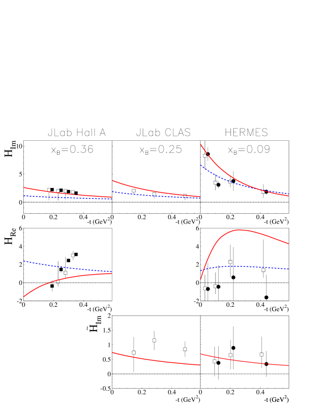
Figure 38: The $H_{Im}$, $H_{Re}$ and $\tilde{H}_{Im}$ CFFs as a function of $-t$ for three different $x_{B}$ values. The empty squares show the results of the 7 CFFs free parameters fit of Refs. [126, 127, 128, 129]. The solid circles in the HERMES column show the result of the linear mapping fit discussed in section 4.2.2 (Ref. [112]). The solid squares in the JLab Hall A column show the result of the $H$-only CFF fit discussed in section 4.2.3 (Ref. [125]). The solid red curves show the result of the VGG model (with $b_{val}=b_{sea}$=1 and without any D-term for $H$). The solid dashed blue curves show the results of the model-based fit of Ref. [113].

In Fig. 38, the results of all these fits are compiled and shown as empty squares (along with and model curves and the rsults of the other fitting strategy that we discuss in the remaining of this subsection). Although error bars are large and the kinematics are not exactly the same between CLAS and the Hall A, it is interesting to note in the case of $H_{Im}$, that one extracts compatible values from fitting different observables (unpolarized and beam-polarized cross sections for Hall A and beam spin and longitudinally polarized target asymmetries for CLAS). One can also note that in this method a better precision on the extraction of $H_{Im}$ is achieved by fitting two asymmetries than two cross sections.

In Fig. 38, some general features and trends can be distinguished:

• Concerning $H_{Im}$, it appears that, at fixed $-t$, it increases as $x_{B}$ decreases (i.e. going from JLab to HERMES kinematics). It is actually possible to extract $H_{Im}$ at the quasi-common value of $-t\approx$ 0.28 GeV² from the JLab Hall A, CLAS and HERMES data (with a slight interpolation in some cases). We then see in Fig. 39, the $x_{B}$-dependence of $H_{Im}$ at $-t\approx$ 0.28 GeV². One observes the rise of this CFF as $x_{B}$ decreases which is similar to the rise of PDFs (due to sea quarks). We recall that $H_{Im}$ reduces to a PDF at $\xi$=0 and $t=0$ GeV². In this figure, we also display the prediction from the VGG (solid red curve) and KM (dashed blue curve) models for $H_{Im}$ CFF at $-t=0.28$ GeV².

• Another feature concerning $H_{Im}$ is that its $t-$slope seems to increase with $x_{B}$ decreasing. We recall that the $t$-slope of the GPD is related to the transverse spatial densities of quarks in the nucleon via a Fourier transform (see Eq. (12)). This evolution of the $t$-slope with $x_{B}$ could then suggest that low-$x$ quarks (the “sea”) would extend to the periphery of the nucleon while the high-$x$ (the “valence”) would tend to remain in the center of the nucleon. We will come back to this discussion in section 6.

• $H_{Re}$ has a very different $t$-dependence than $H_{Im}$ both at JLab and at HERMES energies: while $H_{Im}$ decreases with $-t$ increasing, $H_{Re}$ increases (at least up to $-t\approx$ 0.3 GeV²) and may even change sign, starting negative at small $-t$ and reaching positive values at larger $-t$. The VGG model (red solid curve), as well as the results of the other fitting strategy that we will discuss in the next subsection (solid squares) show or tend to show this “zero-crossing” at JLab kinematics. However, the KM model does definitely not. Given the large error bars on the fitted $H_{Re}$, one cannot at this stage clearly favor or exclude any of the VGG or KM models. These two models have drastically different predictions for this CFF and more precise data on $H_{Re}$ are eagerly asked for.

• Concerning $\tilde{H}_{Im}$, we notice that it is in general smaller than $H_{Im}$, which can be expected for a polarized quantity compared to an unpolarized one. There is very little $x_{B}$ dependence The $t$-dependence of $\tilde{H}_{Im}$ is also rather flat. The weaker $t$-dependence of $\tilde{H}_{Im}$ compared to $H_{Im}$ suggests that the axial charge (to which the $\tilde{H}$ GPD is related) has a narrower distribution in the nucleon than the electromagnetic charge. We remark that the slope of the axial FF (the first $x$-moment of the $\tilde{H}_{Im}$ GPD) is also well known to be flatter compared to those of the electromagnetic FFs. It is very comforting that by studying two relatively different experimental processes (DVCS and for instance $\pi$ production from which the axial FF is in general extracted), one finds similar features. One can also note that there is very little $x_{B}$ dependence for $\tilde{H}_{Im}$ .

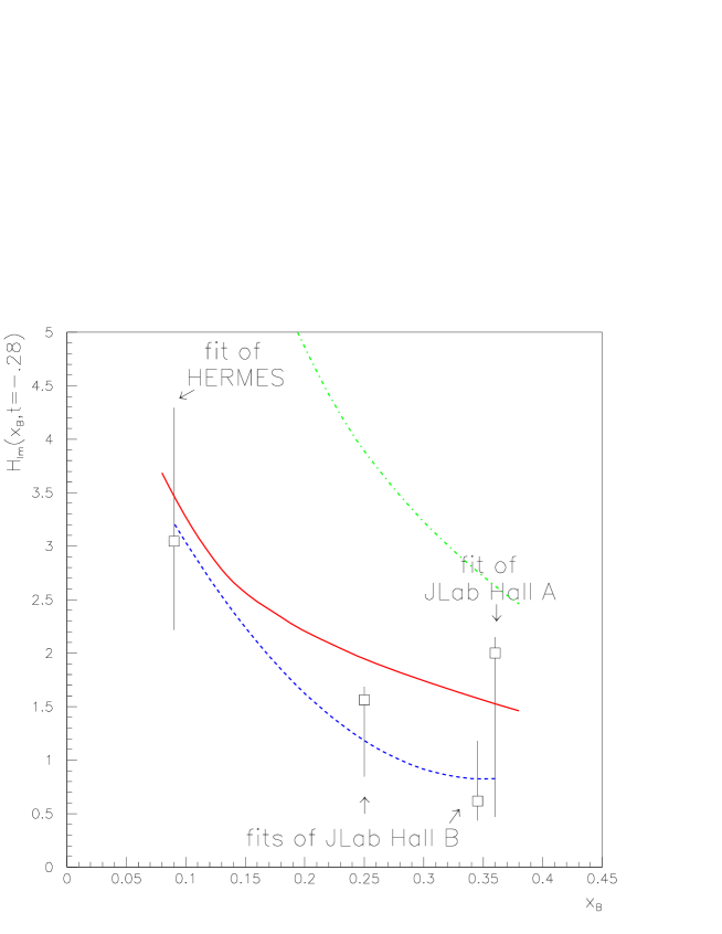
Figure 39: The $H_{Im}$ CFF at $-t\approx 0.28$ GeV² as a function of $x_{B}$. The empty squares show the result of the 7 CFFs free parameters fit from Refs. [126, 127, 128, 129]. The point at $x_{B}\approx$ 0.09 is from the fit of the HERMES data, the ones at $x_{B}\approx$ 0.25 and 0.35 from the fit of the CLAS data and the one at $x_{B}\approx$ 0.36 from the fit of the JLab Hall A data. The solid red curves show the result of the VGG model (with $b_{val}=b_{sea}$=1 and without any D-term for $H$). The solid dashed blue curves show the results of the model-based fit of Ref. [113]. The dash-dotted green curve shows the result of $H_{Im}$ at $-t=0$ GeV², i.e. the PDF (MRST02).

4.2.2 Mapping and linearization

In Ref. [112], a more elegant method has been developped. It consists in establishing a set of relations associating the DVCS observables to the CFFs. This is called “mapping”. Given some reasonable approximations (DVCS leading-twist and leading-order dominance, neglect of some $\frac{t}{Q^{2}}$ terms in the analytical expressions, …), these set of relations can be linear. Eqs. 31 give four examples of such relations. All others can be found in Ref. [55]. Then, if a quasi-complete set of DVCS experimental observables can be measured at a given ($x_{B}$, $Q^{2}$, $-t$) point, one can build a system of eight linear equations with eight unknowns, i.e. the eight CFFs.

Such system can be solved rather straightforwardly with standard matrix inversion and covariance error propagation techniques. This approach has been applied in Ref. [112] to the HERMES data. We recall that HERMES has this unique characteristic to have measured all beam-target single- and double-spin DVCS observables. The absence of cross section measurement at HERMES means however that these spin observables are actually under the form of asymmetries, i.e. a ratio of polarized cross sections to unpolarized cross sections of the form $\frac{\Delta\sigma}{\sigma}$. This has the consequence that the mapping is not fully linear and that some additionnal (reasonable) approximations have to be made such as the dominance of the BH squared amplitude over the DVCS squared amplitude.

With an appropriate selection (with some partial redefinition) of eight HERMES observables, the others serving as consistency checks, the authors of Ref. [112] has been able to solve the system of eight equations and extract the eight CFFs with their uncertaintities. In this well-constrained approach, the uncertaintities on the CFFs reflect essentially the errors of the experimental data. Fig. 38 shows the results of this mapping technique for the three CFFs $H_{Im}$, $\tilde{H}_{Im}$ and $H_{Re}$ in the HERMES column (black circles). With the precision of the HERMES data, only the $H_{Im}$ CFF come out to be clearly different from zero, all others CFFs being compatible with zero within error bars.

In Fig. 38, the agreement of the mapping technique with the “brute force” least-square minimization technique discussed in the previous section is striking (we note that the least-square minimization technique was also applied in Ref. [112], with results well in agreement with those of Ref. [128]). We refer the reader to Ref. [112] for a discussion on the reason why the error bar on $H_{Im}$ for the third $t$ value (around -.2 GeV²) is somewhat larger than for the other $t$ values. We also note that HERMES measured the $A_{UL}$ asymmetry at four $t$ values which should therefore allow in principle to extract $\tilde{H}_{Im}$ at these four $t$ values. However, the extracted $\tilde{H}_{Im}$ CFF at the lowest $\mid t\mid$ point (around -.03 GeV²) turns out to be negative (although compatible with zero within two standard deviations, which does not discard a statistical fluctuation effect). This is both in the present mapping approach and in the least-square minimization approach discussed in the previous section. This negative value for $\tilde{H}_{Im}$ at very low $\mid t\mid$ is a bit surprising as, unless skewdness effects introduce a sign flip, it would imply a negative proton polarized parton distribution function. We do not display it here but it is shown in Ref. [112].

4.2.3 Fitting with only $H$

One limitation of the two previous methods that we just presented is that every ($E_{e},x_{B},Q^{2},t$) kinematic point is taken individually and fitted independently of all others, in particular of its neighbors which have no influence on the fit. On the considered experimental data sets, it turns out that the resulting CFFs display a rather smooth behavior as a function of $-t$ and don’t show oscillations. This, in a way, validates the method but nothing prevents the occurrence of oscillations when studying other measurements. Still, one could wish to improve the procedure and, staying in an almost model-independent fitting framework, enforce some general properties like the smoothness or continuity of the CFFs or the implementation of dispersion relations.

One attempt to enforce the smoothness of the CFFs was made in 2009 in Ref. [125], working with the CLAS beam spin asymmetries and the JLab Hall A unpolarized and beam-polarized cross sections and assuming the dominance of the GPD $H$. As we saw in section 4.1, this assumption is supported by all models and is expected to work at the 20 to 50 % accuracy. In Ref. [125], this influence of the other GPDs was probed by fitting the data assuming that $E$, $\tilde{H}$ and $\tilde{E}$ either vanish or take their VGG values, and studying the dispersion of the fit results.

To enforce the smoothness, one imposes a generic functional form to the $H$ GPD. In Ref. [125], the singlet combination $H_{+}$ is parameterized in the dual model framework according to Eq. (LABEL:eq:duale) (the GPD $E$ is neglected). The $t$-dependence of the $B_{nl}$ coefficients is parameterized as:

$$B_{nl}(t,Q^{2}_{0})=\frac{a_{nl}}{1+b_{nl}(t-t_{0})^{2}}$$ (138)

with $t_{0}$ = - 0.28 GeV². Such a parameterization correlates the $x$ and $t$ dependences. The reference scale is defined by $Q_{0}^{2}$ = 3 GeV² and the $Q^{2}$ evolution is performed with 3 active quark flavors and $\Lambda$ = 373  MeV.

The convergent series Eq. (91) is truncated at some maximal value of $N_{\textrm{max}}$. A rough estimate of the uncertainty related to the specific choice of the truncation was obtained by comparing fit results with different values of $N_{\textrm{max}}$. Choosing $N_{\textrm{max}}$ = 2, 3 or 4 is sufficient to obtain reasonable fits to the data. Larger values of $N_{\textrm{max}}$ produce numerical instability with some coefficients left largely undetermined; the overall quality of the fit also becomes poor.

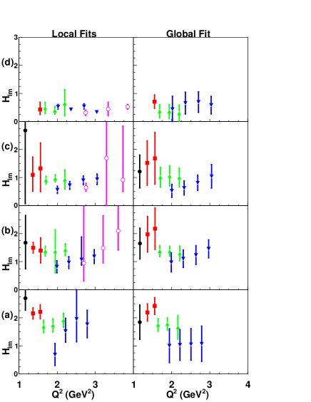
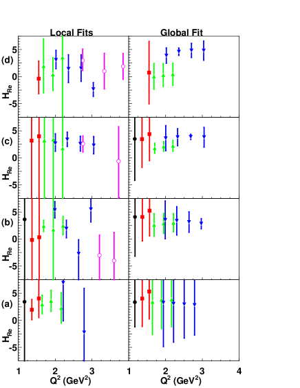
Figure 40: $Q^{2}$-behavior ($1<Q^{2}<4~{}\textrm{GeV}^{2}$) of the extracted values of $H_{Im}$ and $H_{Re}$ of local fits (left) and global fit (right) on Hall B kinematics : $0.09<-t<0.2~{}\textrm{GeV}^{2}$ (a), $0.2<-t<0.4~{}\textrm{GeV}^{2}$ (b), $0.4<-t<0.6~{}\textrm{GeV}^{2}$ (c), and $0.6<-t<1.~{}\textrm{GeV}^{2}$ (d). The error bars include both statistics and systematics. $H_{Im}$ ranges between 0 and 10, $H_{Re}$ between -7.5 and +7.5. Note the change of notational conventions with respect to Eq. (19) and Eq. (23) to match the results published in ref. [125]. The black full circles correspond to $x_{B}$=0.125, red squares to $x_{B}$=0.175, green up triangles to $x_{B}$=0.250, blue down triangles to $x_{B}$=0.360 and magenta open circles to $x_{B}$=0.491.

The fits to the Hall A and CLAS data were performed in two ways: either “locally”, i.e. fitting each individual kinematic bin ($E_{e},x_{B},Q^{2},t$) independently of the other, as described in previous section, or “globally”, i.e. fitting all ($E_{e},x_{B},Q^{2},t$) kinematic bins simultaneously. The left and right panels of Fig. 40 display the results for the $H_{Im}$ and $H_{Re}$ CFFs respectively, for both methods. The results for both kinds of fits are almost always compatible, which is a good consistency check. As expected, the results of the global fits are in general smoother, due to the implementaton of the functional form for $H$. This is especially true concerning $H_{Re}$ : in the case of the local fits, this CFF shows large fluctuations between neighboring bins, with in some cases values falling even outside the plot range. The results of the local fits suffer from large fluctuations as the fits are not constrained enough in some bins but have the advantage of being almost model-independent.

Both local and global fits give results with comparable accuracy for $H_{Im}$. While $H_{Im}$ is rather precisely extracted, $H_{Re}$ is still poorly known, which was also a conclusion of section 4.2.1.

4.2.4 Neural networks

For the sake of completeness, we finally mention the pioneering work Ref. [130] which constitutes the first attempt to extract CFFs from DVCS data with neural networks instead of traditional least square minimization methods. We will not cover it in details since it deals only with a subset of existing data, namely HERMES beam spin and beam charge asymmetries. This approach yields uncertainties in agreement with those obtained from fits with an a priori given functional form and standard statistical procedures. Being largely model-independent, the uncertainties estimated when extrapolating to the $t\rightarrow 0$ region are presumably safer. This body of results will certainly trigger new studies in the future.

5 The future

So far, the data relevant to the DVCS physics in the valence region have come from the JLab Hall A and CLAS experiments using a 6 GeV electron beam and from the HERMES experiment using a 27 GeV electron or positron beam. As described in detail above, Hall A has measured unpolarized and beam-polarized cross sections [58], CLAS beam spin asymmetries and longitudinally target spin asymmetries [61] and HERMES the complete set of beam charge, beam spin and target spin asymmetries [64, 65, 66, 67, 68, 69, 70, 71]. We have made use of practically all these existing data in the previous sections by comparing them to model calculations or fitting them in order to extract CFFs. These data have allowed to show the successes and the limits of the present GPD parameterizations and to develop the first GPD of CFF fitter codes. Putting together all these informations, one can consider that the $H_{Im}$ CFF is relatively well constrained and known at the $\approx$15% level and that some first constraints on the $\tilde{H}_{Im}$ and $H_{Re}$ CFFs start to appear.

Although possibly more information can still be extracted from these data, one clearly wishes to have, ideally, more observables, more precise data and a larger phase space coverage. In the intermediate $x_{B}$ region ($\approx$ 0.1), unfortunately not much more can be expected from HERMES since the experiment has shut down a few years ago. However, the COMPASS experiment with a 160 GeV muon beam is scheduled to have around 2016 a dedicated DVCS program with a specific recoil detector to ensure the exclusivity of the process [131]. It should then be able to explore the $x_{B}$ range between $0.01$ and $0.1$, thus with some partial overlap with HERMES.

On a shorter time scale, a lot of new data are expected to come from JLab. The 6 GeV era has just finished in summer 2012 and many data are currently under analysis:

• In Hall A, the experiment E07-007 [132] has carried out DVCS measurements at two beam energies (6 and 4 GeV) for which it is planned to extract the unpolarized and beam-polarized cross sections. At fixed $x_{B}$ and $Q^{2}$, the beam energy dependence, analog to a Rosenbluth separation, will allow to separate the pure DVCS contribution from the BH-DVCS interference contribution. Strong contraints on the real CFFs, in particular $H_{Re}$, are expected from this measurement.

• With CLAS, the experiment E06-003 [133] has carried out DVCS measurements at $\approx$ 6 GeV with a polarized beam. A first set of beam spin asymmetries released of this experiment has already been published [61] and discussed in the previous sections but another set with double statistics is currently under analysis. Most importantly, unpolarized and beam-polarized cross sections are in the process of being extracted. A glimpse on these cross sections is available in Ref [60]. These cross sections are expected to be less precise than the Hall A ones due to the systematic uncertainties inherent to a large acceptance detector such as CLAS. However, they will cover a much larger phase space. Strong constraints on the $H_{Re}$ and $H_{Im}$ are expected from this measurement.

• With CLAS, the experiment E05-114 [134] has carried out DVCS measurements at $\approx$ 6 GeV with a longitudinally polarized proton (and neutron) target and a polarized beam. Improved $A_{UL}$ (w.r.t. Ref. [63]) and, for the first time, $A_{LL}$ measurements are thus expected soon. This will allow to further constrain the $\tilde{H}_{Im}$ CFF in particular.

JLab is currently in an upgrade phase and plans to deliver a 12 GeV beam around 2015. A DVCS program in Hall A and in CLAS has already been approved:

• In Hall A, the experiment E12-06-114 [135] will measure the unpolarized and beam-polarized cross sections in a new kinematical regime (smaller $x_{B}$ and larger $Q^{2}$).

• With CLAS, the experiment E12-06-119 [136] will use a polarized beam and a longitudinally polarized target to measure unpolarized cross sections and beam spin, target spin and double spin asymmetries.

• With CLAS, the proposal C12-12-010 [137] aims at measuring the DVCS reaction with a tranversally polarized target. This should bring strong constraints on the $E$ GPD (see Eq. (34)).

• Besides the DVCS experiments off the proton, the experiment E12-12-003 [138] aims at measuring DVCS on the neutron. Except for the pioneering measurement of the Hall A [59], DVCS on the neutron has never been measured. It is obviously an indispensable process to measure in order to perform a flavor separation of the GPDs.

Fig. 41 compares the ($x_{B}$,$Q^{2}$) domains that are explored or will be explored by JLab 12 GeV, HERMES, COMPASS and H1/ZEUS regarding the DVCS and DVMP processes. This illustrates the complementarity of all these facilities, the near future belonging to the JLab 12 GeV and COMPASS facilities. In the following two sections, we show some examples of what is expected to be achieved with the JLab 12 GeV facility and in the third one a comparison of the predictions for the various models presented and discussed in sections 3 and 4 for COMPASS kinematics.

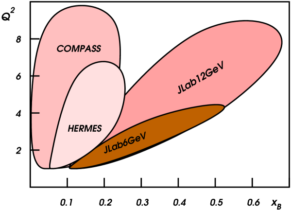
Figure 41: ($x_{B}$,$Q^{2}$) domain explored by JLab 12 GeV, HERMES and COMPASS regarding the DVCS (the limits take into a $W>$2 GeV cut and an approximate estimation of the luminosity of each facility).

5.1 Hall A

While the CLAS12 detector will explore a wide phase space region for the DVCS process, the DVCS program in Hall A will be to focus on some specific kinematics and make precision measurements. In terms of systematic uncertainties, we recall that the typical momentum resolution of the Hall A arm spectometers is of the order of $10^{-4}$ (compared to $10^{-2}$ for CLAS12) and that, in terms of statistics, the luminosity that can be reached in Hall A is of the order of $10^{38}cm^{-2}s^{-1}$ (compared to $10^{35}cm^{-2}s^{-1}$ for CLAS12). In particular, before thinking of extracting GPDs or CFFs out of DVCS data, it is of the utmost importance to ensure that the “handbag” formalism is applicable, in particular at the relatively low $Q^{2}$ values that can be reached at JLab. One of the signatures to be looked for is the scaling behavior of the CFFs, i.e. the property that they don’t depend on $Q^{2}$ at leading-twist.

The preliminary tests of scaling carried out at 6 GeV by the Hall A collaboration are encouraging (see Fig. 13) but are limited in the $Q^{2}$ range (between 1.4 and 2.4 GeV²). Fig. 42 shows the gain in the $Q^{2}$ range that can be obtained with the JLab 12 GeV beam energy increase. The errors on this figure were estimated for 90 days of beam time and the running conditions of the JLab Hall A proposal [135].

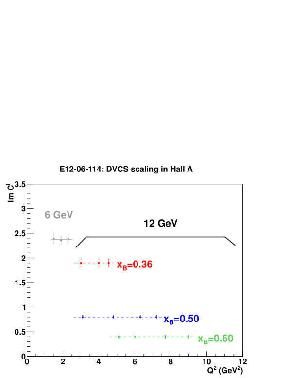
Figure 42: Projected uncertainties from the JLab 12 GeV Hall A E12-06-114 experiment [135] for the $Q^{2}$-dependence of the $H_{Im}$ CFF for different $x_{B}$ (figure done by C. Munoz).

5.2 CLAS12

CLAS12 is expected to measure all the DVCS observables accessible with a polarized beam, a longitudinally and a transversely polarized target. Except for beam charge observables, this makes up for a complete program. In this section, we show what can be achieved in terms of the extraction of CFFs using the technique presented in section 4.2.1. This study has been done in collaboration with H. Avakian.

For each ($x_{B}$, $Q^{2}$, $t$) bin, the $\phi$ distributions of the various independent DVCS spin observables which are measurable with a longitudinally polarized beam and a longitudinally or/and transversely polarized proton target, have been generated: $A_{LU}$, $A_{UL}$, $A_{LL}$, $A_{Ux}$, $A_{Uy}$, $A_{Lx}$, $A_{Ly}$ (in addition to the unpolarized cross section). The VGG values [82] for the four GPDs $H$, $E$, $\tilde{H}$ and $\tilde{E}$ have been used to generate these distributions. Then, $ep\to ep\gamma$ events generated according to the BH+DVCS cross sections have been fed into a fast Monte-Carlo simulating the CLAS12 acceptance and efficiency. Assuming 80 days of beam time for the unpolarized target run at a luminosity of 10³⁵ mc^-2s^-1 (from which the unpolarized cross section and $A_{LU}$ are planned to be extracted), 100 days of beam time for the longitudinally polarized target run at a luminosity of 2.10³⁵ mc^-2s^-1 (from which $A_{UL}$ and $A_{LL}$ are planned to be extracted), 100 days of beam time for the transversely polarized target run at a luminosity of 5.10³³ mc^-2s^-1 (from which $A_{Ux}$, $A_{Uy}$, $A_{Lx}$ and $A_{Ly}$ are planned to be extracted) and furthermore assuming 80% target polarization, one can assign (statistical) error bars to the $\phi$ distributions and then fit them. The goal is to extract the seven CFFs : $H_{Re}$, $E_{Re}$, $\tilde{H}_{Re}$, $\tilde{E}_{Re}$, $H_{Im}$, $E_{Im}$, $\tilde{H}_{Im}$. As already mentioned in section 4.2.1, $\tilde{E}_{Im}$=0 is set to 0 in this study.

Figure 43: Resulting $H_{Re}$ CFF from the simultaneous fit of $A_{LU}$, $A_{UL}$, $A_{LL}$, $A_{Ux}$, $A_{Uy}$, $A_{Lx}$, $A_{Ly}$ and of the unpolarized cross section, for each ($x_{B}$, $Q^{2}$, $t$) bin with the fitting code of Refs. [126, 127, 128, 129]. The extracted CFFs for which the error bar was larger than 3 were removed. (study done in collaboration with H. Avakian).

Figure 44: Resulting $H_{Im}$ CFF from the simultaneous fit of $A_{LU}$, $A_{UL}$, $A_{LL}$, $A_{Ux}$, $A_{Uy}$, $A_{Lx}$, $A_{Ly}$ and of the unpolarized cross section, for each ($x_{B}$, $Q^{2}$, $t$) bin with the fitting code of Refs. [126, 127, 128, 129]. The extracted CFFs for which the error bar was larger than 150% were removed. (study done in collaboration with H. Avakian).

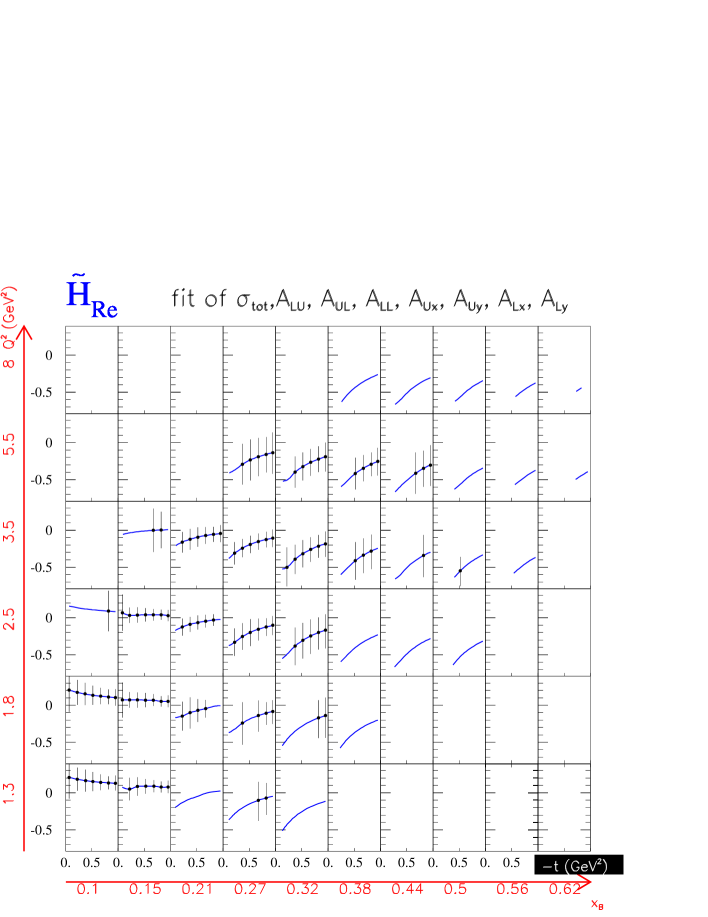
Figure 45: Resulting $\tilde{H}_{Re}$ CFF from the simultaneous fit of $A_{LU}$, $A_{UL}$, $A_{LL}$, $A_{Ux}$, $A_{Uy}$, $A_{Lx}$, $A_{Ly}$ and of the unpolarized cross section, for each ($x_{B}$, $Q^{2}$, $t$) bin with the fitting code of Refs. [126, 127, 128, 129]. The extracted CFFs for which the error bar was larger than 0.3 were removed. (study done in collaboration with H. Avakian).

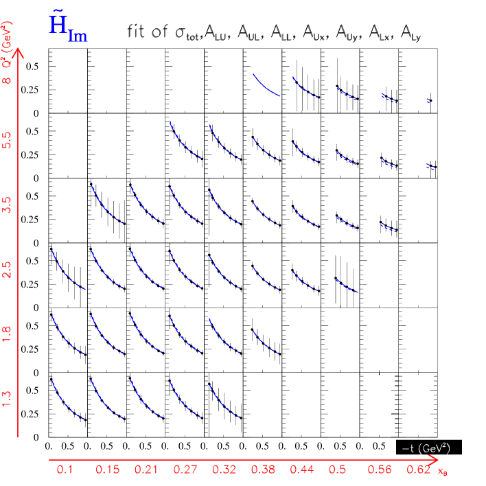
Figure 46: Resulting $\tilde{H}_{Im}$ CFF from the simultaneous fit of $A_{LU}$, $A_{UL}$, $A_{LL}$, $A_{Ux}$, $A_{Uy}$, $A_{Lx}$, $A_{Ly}$ and of the unpolarized cross section, for each ($x_{B}$, $Q^{2}$, $t$) bin with the fitting code of Refs. [126, 127, 128, 129]. The extracted CFFs for which the error bar was larger than 150% were removed. (study done in collaboration with H. Avakian).

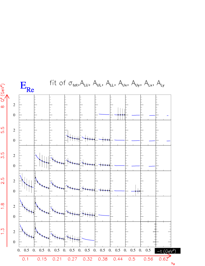
Figure 47: Resulting $E_{Re}$ CFF from the simultaneous fit of $A_{LU}$, $A_{UL}$, $A_{LL}$, $A_{Ux}$, $A_{Uy}$, $A_{Lx}$, $A_{Ly}$ and of the unpolarized cross section, for each ($x_{B}$, $Q^{2}$, $t$) bin with the fitting code of Refs. [126, 127, 128, 129]. The extracted CFFs for which the error bar was larger than 1.5 were removed. (study done in collaboration with H. Avakian).

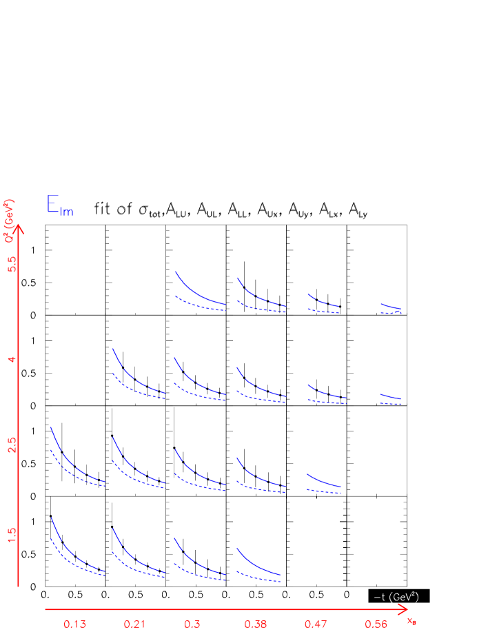
Figure 48: Resulting $E_{Im}$ CFF from the simultaneous fit of $A_{LU}$, $A_{UL}$, $A_{LL}$, $A_{Ux}$, $A_{Uy}$, $A_{Lx}$, $A_{Ly}$ and of the unpolarized cross section, for each ($x_{B}$, $Q^{2}$, $t$) bin with the fitting code of Refs. [126, 127, 128, 129]. The extracted CFFs for which the error bar was larger than 150% were removed. (study done in collaboration with H. Avakian).

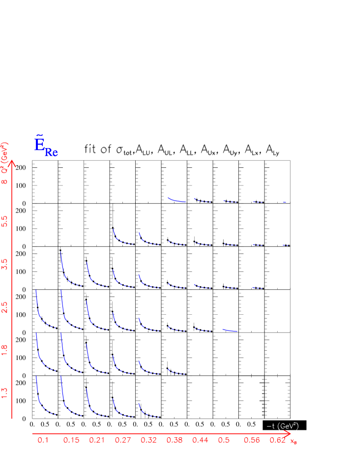
Figure 49: Resulting $\tilde{E}_{Re}$ CFF from the simultaneous fit of $A_{LU}$, $A_{UL}$, $A_{LL}$, $A_{Ux}$, $A_{Uy}$, $A_{Lx}$, $A_{Ly}$ and of the unpolarized cross section, for each ($x_{B}$, $Q^{2}$, $t$) bin with the fitting code of Refs. [126, 127, 128, 129]. (study done in collaboration with H. Avakian).

The results for the seven CFFs issued from the simultaneous fitting of the $\phi$ distribution of $A_{LU}$, $A_{UL}$, $A_{LL}$, $A_{Ux}$, $A_{Uy}$, $A_{Lx}$, $A_{Ly}$ and of the unpolarized cross section with the procedure of Refs. [126, 127, 128, 129] are displayed, for all ($x_{B}$, $Q^{2}$, $t$) bins in Figs. 43 to  49. The reconstructed CFFs with error bars should be compared to the generated ones which are represented by the solid curve. The panels where there are blue solid curves and not CFF reconstructed means that the particular fitting code that we have used was not able to reconstruct the CFFs reliably. In Figs. 43 to  49, we have indeed not plotted the extracted CFFs for which the error bar was too large (see the captions of the figures was the detailed criteria). This does not mean that there are no data reconstructed in those bins. Other fitting algorithms (probably with some model-dependent inputs) can certainly make use of these data and extract some constraints on the CFFs and GPDs.

The dashed curves on the imaginary parts of the CFF plots show the corresponding values of the GPDs for zero skewness argument, i.e. $H(x,0,t)$, $\tilde{H}(x,0,t)$ and $E(x,0,t)$, according to VGG. These latter are the quantities which have a simple probability interpretation. One therefore sees from these (model-dependent) curves, showing the difference between $H(x,x,t)$ and $H(x,0,t)$, the effect of the skewness. We will come back to this issue in the section 6.

With such complete experiments, which comprise all DVCS observables except for beam charge asymmetry, we observe that the seven CFFs can be reconstructed for essentially all ($x_{B}$, $Q^{2}$, $t$) bins with quite good precision. In particular, the measurement of the transverse target spin observables is crucial to reconstruct the CFFs related to the GPD $E$. The same study without such observables allows the reconstruction of the CFFs related to the GPDs $H$ and $\tilde{H}$ only, leaving the CFF $E_{Im}$ practically unconstrained.

In Sec. 2.2 and Sec. 4.1 we already insisted on the required accuracy in the determination of the kinematics of observables. The BH cross section varies strongly when the outgoing photon is emitted in the direction of the incoming or scattering electron. An variation of 1 % in $x_{B}$ can induce a variation of 10 % in the cross section. This has some important consequences regarding the CFF fitting method described above. For the CFFs to be accurately reconstructed, it is necessary to have a complete set of observables on the same ($x_{B}$, $Q^{2}$, $t$) bin. If this is not the case, we have to work with neighboring bins (for example with similar, but not equal $x_{B}$); this approximation will generate a systematic uncertainty on the reconstruction of CFFs that can be quite large.

5.3 COMPASS

The COMPASS experiment plans to measure the correlated beam charge-spin observables:

$$S_{CS,U}=\sigma^{+\leftarrow}+\sigma^{-\rightarrow},$$ (139)

$$D_{CS,U}=\sigma^{+\leftarrow}-\sigma^{-\rightarrow}$$

since the muons of the beam originate from pions decays which induces a correlation between the charge and the spin of the muons.

In Fig. 50, we show the predictions of the four models which we discussed in sections 3 and 4, i.e. the VGG, GK, dual parameterization and KM models. Calculations have been done for $E_{\mu}$=160 GeV, $x_{B}$=0.05, $Q^{2}$=2 GeV² and $-t$=-0.2 GeV². All four models show relatively similar features. The differences lie in the global normalization of the $S_{CS,U}$ observable and in the behavior at the lowest and largest $\phi$ values of the $D_{CS,U}$ observable.

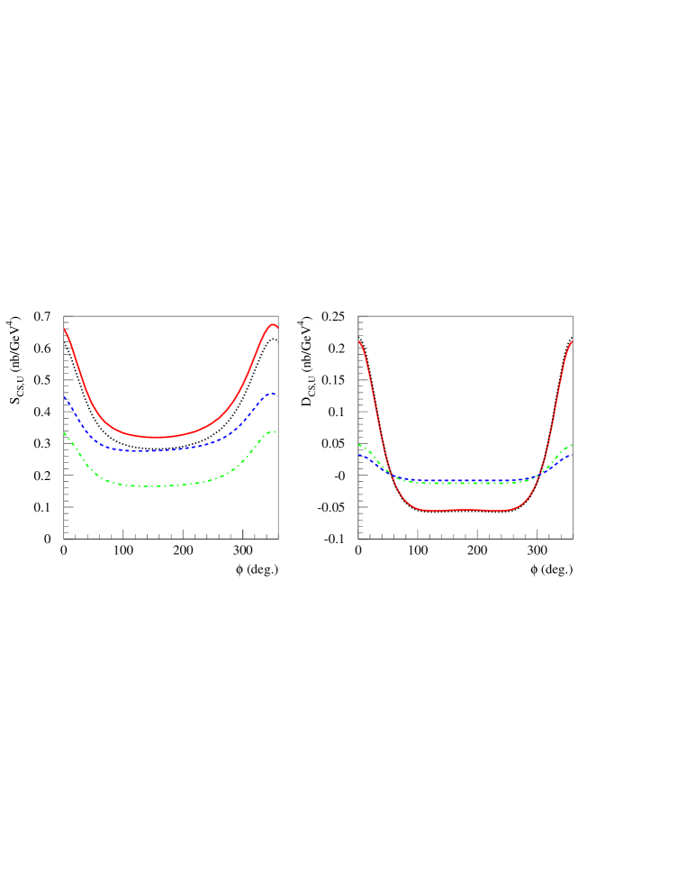
Figure 50: Predictions at $E_{\mu}$=160 GeV, $x_{B}$=0.05, $Q^{2}$=2 GeV² and $-t$=-0.2 GeV² for the $\phi$-dependence of $S_{CS,U}$ (left panel) and $D_{CS,U}$ (right panel) as defined in Eq. 139. Solid red curve: VGG; dashed blue line: GK; dotted black: dual model; dot-dashed green: KM model.

6 From Compton Form Factors to spatial densities

As described above, the GPDs at $\xi=0$, e.g. $H(x,0,t)$, are mapping out the combined probabilities in transverse position and longitudinal momentum of the quarks in the nucleon (see Eq. (12)). We saw in the previous section that CLAS12 will allow to essentially extract all CFFs, with more or less precision depending on the CFF and the kinematics, over the range $0.1\lesssim x_{B}\lesssim 0.6$ and $t_{min}\lesssim-t\lesssim 1$ GeV². In particular, if we focus on the unpolarized GPD $H$, the CFF $H_{Im}=H(\xi,\xi,t)-H(-\xi,\xi,t)$ can be extracted quite precisely. In the following, in this pioneering exercise, we will make the approximation of neglecting the antiquark contribution to the $H_{Im}$ CFF, i.e. neglect $H(-\xi,\xi,t)$ w.r.t. $H(\xi,\xi,t)$. At CLAS kinematics, according to the GK and VGG models, $H(-\xi,\xi,t)$ is about 20% of $H_{Im}$ while at HERMES kinematics, it is about 30%. This approximation being clearly set, given the uncertainties on $H(\xi,\xi,t)$, and modulo a (model-dependent) skewness correction of the form $H(\xi,0,t)/H(\xi,\xi,t)$, one can adress several questions :

• With which accuracy can one extract $H(x,b_{\perp})$ from the measurement of the diagonal CFF $H(\xi,\xi,t)$ ?

• How does one perform such error propagation ?

• What is the model dependence of the skewness correction ?

Eq. (12) can be equivalently expressed, for a circularly symmetric function, through the Hankel transform:

$$H(x,b_{\perp})=\int\limits_{0}^{\infty}\frac{d\Delta_{\perp}}{2\pi}\,\Delta_{\perp}\,J_{0}(b_{\perp}\Delta_{\perp})\,H(x,0,-\Delta_{\perp}^{2}),$$ (140)

where $\Delta_{\perp}\equiv|{\bf\Delta}_{\perp}|$, and $J_{0}$ is the Bessel function of order 0.

We present here a simple numerical algorithm which adresses the error propagation in this transform. We illustrate it by focusing on $H_{Im}$ and by taking one particular $(x_{B},Q^{2})$ bin in Fig. 44, e.g. $(0.1,2.5$ GeV²). Fig. 51 (left panel) displays the pseudo-data and the associated errors contained in this bin. The procedure consists in smearing “vertically” the seven values of $H(\xi,\xi,t)$ (which correspond to seven $t$ values) according to a Gaussian distribution with a standard deviation equal to the error bar of the point. These 7 “new” points are then fitted by a function, which we take as an exponential $Ae^{Bt}$ with two free parameters, the normalization $A$ and the slope $B$. At fixed $x_{B}$, an exponential ansatz is motivated by most GPD models (for instance VGG, GK, KM,… which we discussed in section 3). In principle, any other fit function can be used, and can serve as a way to estimate a systematic uncertainty associated to this method. This procedure (smearing + fitting) is repeated several thousand times so that one obtains several thousand exponential functions, shown in Fig. 51 (middle panel).

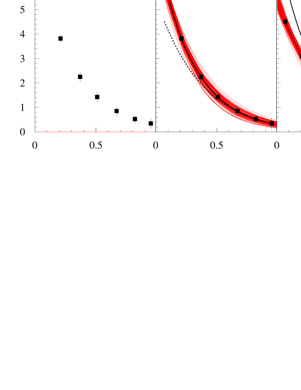
Figure 51: Left: pseudo-data for the $t$-distribution of the $H_{Im}$ CFF (zoom of the $(x_{B},Q^{2})$ bin $(0.1,2.5$ GeV²) of Fig. 44). Middle: same as left figure with, superposed, the series of $Ae^{Bt}$ red curves fitting the smeared pseudo-data. The solid black curve shows the VGG $H_{Im}$ CFF, i.e. $H(\xi,\xi,t)$. The dashed black curve shows the VGG value for $H(\xi,0,t)$. Right: same as left figure with, superposed, the series of $Ae^{Bt}$ red curves fitting the smeared pseudo-data, where these latter have been corrected by $H(\xi,0,t)/H(\xi,\xi,t)$.

Then, each of these several thousand exponentials is transformed through Eq. (140) so that one obtains a series of Hankel transforms, now as a function of $b_{\perp}$. This transform can be done analytically in the present case but any numerical method is also possible if the function fitting $H(\xi,\xi,t)$ does not have a simple Hankel transform. The idea is then to look, for various values of $b_{\perp}$, at the dispersion of all the Hankel transforms. The spread of the Hankel transforms for a few (arbitrarily) selected $b_{\perp}$ values is shown in Fig. 52. One sees that the resulting distributions are quasi-Gaussian. One can therefore fit those distributions by a Gaussian function from which one extracts the mean and the standard deviation. The black points in Fig. 53 show the result of this procedure. The error bars at each $b_{\perp}$ value result from the propagation of the error bars of $H(\xi,\xi,t)$ displayed in Fig. 51. We choose to display here only seven $b_{\perp}$ points but the procedure can be applied to any number of $b_{\perp}$ points so that one can obtain a continuous distribution as a function of $b_{\perp}$. The interest of this method is to properly propagate the errors on $H(\xi,\xi,t)$ to its Hankel transform. In particular, it takes into account the correlations between the parameters used to fit $H(\xi,\xi,t)$ (in the present case, the normalization and the slope of the exponential).

Figure 52: Distributions of the Hankel transforms $H(x=0.053,b_{\perp})$, for selected $b_{\perp}$ values, for the series of fit curves corresponding to the middle panel of Fig. 51. The mean and standard deviation (respectively the parameters P2 and P3 in the inserts of each panel) of the Gaussian fit of these distributions is extracted to obtain the $b_{\perp}$-dependence of the spatial density.

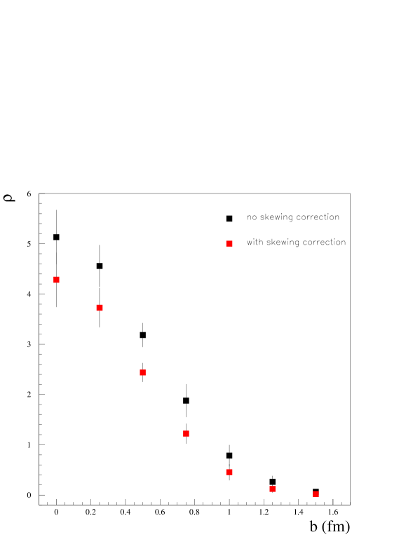
Figure 53: $b_{\perp}$-dependence of the spatial density $H(x=0.053,b_{\perp})$ resulting from the Hankel transform of Fig. 51, middle panel, i.e. without any “deskewing” correction (black points), and of Fig. 51, right panel, i.e. with “deskewing” correction (red points).

However, in order to be able to interpret such distribution as the transverse spatial density of the quarks at the particular value of $x=\xi=0.053$ taken here, a correction needs to be made. So far, we have Hankel-transformed $H(\xi,\xi,t)$. However, the spatial density interpretation requires the knowledge of $H(\xi,0,t)$. The correction to pass from one to the other has to be model-dependent since the $x$ and $\xi$-dependencies cannot be measured independently with the DVCS process. A model-dependent $H(\xi,0,t)/H(\xi,\xi,t)$ skewness correction factor should therefore be applied.

Fig. 54 shows such deskewing correction factor for three models that we discussed in section 3. It is seen that below $-t$=1 GeV², they don’t differ by more than 10%. They all three correspond to a correction of the order of  20% at small t with a similar evolution as $-t$ grows up to 1 GeV². Such comparison between different models can serve to estimate a systematic uncertainty in the deskewing. We note that the deskewing factor depends on $t$ in a similar way for all three models. As $\mid t\mid$ grows, the deskewing factor grows towards one (and can even go over one). This means that it flattens the $t$ slope of $H(\xi,0,t)$ w.r.t. to the measured or extracted $H(\xi,\xi,t)$. All three models also show a similar $x_{B}$-dependence between the CLAS and the HERMES kinematics, i.e. the deskewing correction is less important as $x_{B}$ increases.

We then apply such a deskewing factor to the pseudo-data of our selected ($x_{B}$, $Q^{2}$) bin. This yields the new set of data shown in Fig. 51 (right panel). Then, the procedure that we just described is applied to these “deskewed” data (see the red curves in Fig. 51, right panel). This results in the the $b_{\perp}$ distribution given by the red points in Fig. 53, which can now be properly interpreted as a spatial density. We stress that we place ourselves in a leading twist and leading order framework in this whole exercise.

We have focused so far on one particular $(x_{B},Q^{2})$ bin in order to illustrate the method. We now process a series of $x_{B}$ bins in order to provide an imaging of the nucleon. We select in Fig. 44 the $H_{Im}$ row at $Q^{2}$=2.5 GeV² where there are 7 $x_{B}$ bins (if $Q^{2}$ corrections are under control or found negligible, different $Q^{2}$ rows can of course be combined). Fig. 55 shows the result where we now see the evolution of the transverse spatial density as a function of $x_{B}$. In particular, one notes that, as $x_{B}$ decreases the radius of the proton increases. This is a feature which was implemented in VGG and it serves as a proof of principle that, after the different steps, of computing the DVCS observables from the VGG model, generating the pseudo-data according to these, processing these through a simulation of the CLAS12 detector, fitting these pseudo-data in order to extract the $H_{Im}$ CFF and the final Hankel-transform procedure that we just discussed , one recovers the original features of the VGG model.

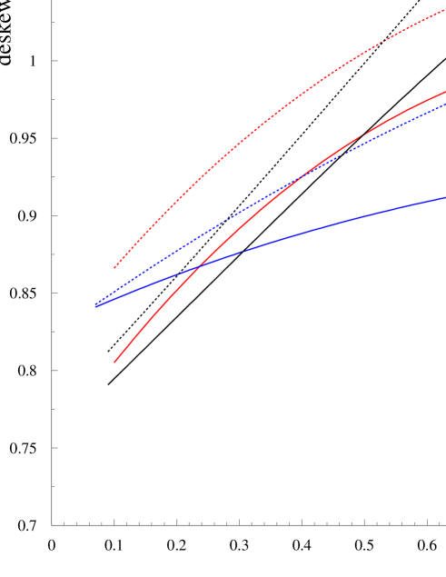
Figure 54: “Deskewing” factor $H(\xi,0,t)/H(\xi,\xi,t)$ as a function of $-t$ for the VGG model (red curves), the GK model (blue curves) and the dual model (black curves). The solid curves correspond to $x_{B}$=0.1 (HERMES kinematics) and the dashed ones to $x_{B}$=0.25 (CLAS kinematics).

Figure 55: Left: Evolution of the $b_{\perp}$-spatial densities as a function of $x_{B}$. The seven curves correspond to the Hankel transforms of the $Q^{2}$=2.5 GeV² row of $H_{Im}$ in Fig. 44. Right: alternative view in color for visibility.

We finally apply this procedure to real data. We recall that $H_{Im}$ has been extracted out of the CLAS and HERMES data (see Fig. 38). Figs. 56 and 57 show the results of the procedure. Of course, the $H_{Im}$ data have much larger error bars than the CLAS12 simulations and the exponential fits (red curves on the left panels of Figs. 56 and 57) have a lot of dispersion. The distribution of the Hankel transforms at fixed $b_{\perp}$ are then not as clean as in Fig. 52. In particular, the fits in Figs. 56 and 57 sometimes are horizontal straight lines (which correspond to exponentials with a zero slope) and this produces double peaks in the $b_{\perp}$ slices. Nevertheless, a dominant Gaussian-like peak always remains distinguishable from which a centroid and a standard deviation can be extracted, yielding the spatial charge densities of Fig. 56 (right panel), corresponding to $x_{B}$=0.25, and Fig. 57 (right panel), corresponding to $x_{B}$=0.09. Given the size of the experimental errors on the $H_{Im}$ data, we choose to ignore in this exercise the uncertainty associated to the deskewing. We also neglect at this stage the uncertainty associated with the fact that the different DVCS-BH asymmetries that are used to extract $H_{Im}$ are given at similar, but not strictly equal, kinematic $(x_{B},t,Q^{2})$ points. This being said, in spite of the large error bars and some uncertainties in the procedure that we ignored, we can distinguish the same features than we observed with the simulations, namely, an increase of the size of the proton with $x_{B}$ decreasing. The overall increase in the normalization of the density is due to the rise of the unpolarized parton distribution function as $x_{B}$ decreases. As a further illustration, we fitted the spatial charge densities of the right panels of Figs. 56 and 57 by a Gaussian function which we plot as contour plots in Fig. 58.

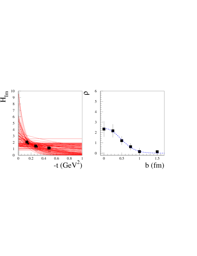
Figure 56: Left: the black squares show $H_{Im}$ extracted without any deskewing correction and the black stars with deskewing correction, from the CLAS data. For visibility, the $t$ values of the squares and stars are slightly shifted around the true $t$ values. The red curves are the fitted $Ae^{Bt}$ functions obtained from the smearing of the $H_{Im}$ points. Right: resulting spatial charge density. The blue dashed curve is the result of a fit by a Gaussian function.

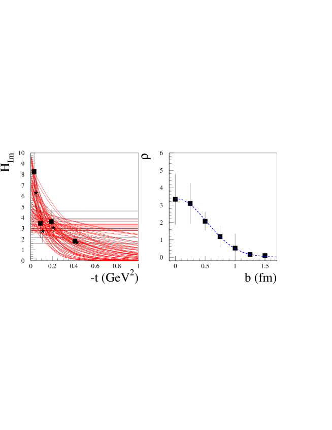
Figure 57: Left: the black squares show $H_{Im}$ extracted without any deskewing correction and the black stars with deskewing correction, from the HERMES data. For visibility, the $t$ values of the squares and stars are slightly shifted around the true $t$ values. The red curves are the fitted $Ae^{Bt}$ functions obtained from the smearing of the $H_{Im}$ points. Right: resulting spatial charge density. The blue dashed curve is the result of a fit by a Gaussian function.

Figure 58: Left: contour plot of the spatial charge density at CLAS kinematics ($x_{B}$=0.25) extracted from Fig. 56. Right: contour plot of the spatial charge density at HERMES kinematics ($x_{B}$=0.09) extracted from Fig. 57.

7 Conclusions and outlook

In this work, we have briefly reviewed the field of the Generalized Parton Distributions and Deeply Virtual Compton Scattering in the valence region, with emphasis on the information which can be extracted from present and forthcoming data. After briefly recalling the theoretical formalism and the properties and interests of the GPDs, we have reviewed the few existing data from the HERMES and JLab facilities. Then, we presented four widely used GPD parameterizations based on different approaches (double distributions, dual parameterization, and Mellin-Barnes representation), followed by a more general discussion of DVCS observables within a dispersion relation framework. In the present work, our study was based on a leading-twist and leading-order QCD assumption. We compared the results of these different approaches to the existing data. We found that, although many features and trends of the experimental observables were correctly accounted for, no model satisfactorily describes simultaneously the full set of current HERMES and JLab data. We also presented an alternative approach of fitting the Compton Form Factors, which are functions of GPDs, in more or less model-independent ways. Given the few existing data, the information that can be extracted in this way is limited but nevertheless brings additional clues on the behavior of GPDs.

Putting all the model-dependent and model-independent pieces of the puzzle together, one can conclude so far that the CFF $H_{Im}$ can be considered as known in the valence region at the $\approx$ 15% level and, to a lesser extent, the CFF $\tilde{H}_{Im}$. We have further shown that an imaging of the nucleon starts to appear from these analyses. One feature which emerges from this analysis is that the increase of the $t$-slope of $H_{Im}$ with decreasing $x_{B}$ is reflecting the increasing transverse size of the nucleon as one probes partons with smaller and smaller momentum fractions (in the so-called light-front frame). This yields an image of the nucleon with a core of valence quarks surrounded by a cloud of quark-antiquarks. Another feature, resulting from the observation that the CFF $\tilde{H}_{Im}$ has a flatter $t$-dependence than the $H_{Im}$ and barely varies with $x_{B}$ is that the axial charge of the nucleon tends to stay concentrated in the core of the nucleon.

Furthermore, we explored the future of the field, in particular by summarizing all the simulation work that has been carried out for the JLab 12 GeV facility. With the upgrade in energy and luminosity (for CLAS) of JLab, an unprecedented set of data in precision and phase-space coverage is anticipated. We showed that essentially all leading-twist CFFs will be extracted, some with better precision than others. In the final chapter of this review, we finally proposed a method to transform a CFF measurement into a spatial charge density measurement with proper error propagation. We applied this technique to the JLab 12 GeV pseudo-data as well as to the few existing data from JLab 6 GeV and HERMES.

The future of the field is bright with numerous new data in perspective from JLab 12 GeV and COMPASS. The few existing data, with their limitations in terms of precision and phase space coverage, allow to develop the techniques (models, fits,…) to be employed in the future. Within the present work, we showed within the leading-twist and leading order QCD assumptions, a proof of principle to extract the GPD related observables from the deeply virtual Compton process. Furthermore, on can anticipate further developments on the theory side in calculating the corrections required by the anticipated precision of the forthcoming data. Such program will allow to image the partonic structure of the nucleon. Visualizing will then deepen our understanding.

References

References

- [1] Burkardt M 2000 Impact parameter dependent parton distributions and off-forward parton distributions for zeta 0 Phys. Rev. D 62 071503
- [2] Burkardt M 2003 Impact parameter space interpretation for generalized parton distributions Int. J. Mod. Phys. A 18 173
- [3] Miller G A 2007 Charge Density of the Neutron Phys. Rev. Lett. 99 112001
- [4] Carlson C E and Vanderhaeghen M 2008 Empirical transverse charge densities in the nucleon and the nucleon-to- transition Phys. Rev. Lett. 100 032004
- [5] Miller G A 2010 Transverse Charge Densities Ann. Rev. Nucl. Part. Sci. 60 1
- [6] Perdrisat C F, Punjabi V and Vanderhaeghen M 2007 Nucleon Electromagnetic Form Factors Prog. Part. Nucl. Phys. 59 694
- [7] Arrington J, Roberts C D and Zanotti J M 2007 Nucleon electromagnetic form factors J. Phys. G 34 S23
- [8] Mueller D, Robaschik D, Geyer B, Dittes F M and Horejsi J 1994 Wave functions, evolution equations and evolution kernels from light ray operators of QCD Fortsch. Phys. 42 101
- [9] Ji X D 1997 Gauge invariant decomposition of nucleon spin and its spin - off Phys. Rev. Lett. 78 610
- [10] de Florian D, Sassot R, Stratmann M and Vogelsang W 2012 QCD Spin Physics: Partonic Spin Structure of the Nucleon Prog. Part. Nucl. Phys. 67, 251
- [11] Ji X D 1997 Deeply virtual Compton scattering Phys. Rev. D 55 7114
- [12] Radyushkin A V 1996 Scaling Limit of Deeply Virtual Compton Scattering Phys. Lett. B 380 417
- [13] Radyushkin A V 1997 Nonforward parton distributions Phys. Rev. D 56 5524
- [14] Collins J C, Frankfurt L and Strikman M 1997 Factorization for hard exclusive electroproduction of mesons in QCD Phys. Rev. D 56 2982
- [15] Anikin I V, Pire B and Teryaev O V 2000 On the gauge invariance of the DVCS amplitude Phys. Rev. D 62 071501
- [16] Radyushkin A V and Weiss C 2001 DVCS amplitude at tree level: Transversality, twist - three, and factorization Phys. Rev. D 63 114012
- [17] Kivel N, Polyakov M V and Vanderhaeghen M 2001 DVCS on the nucleon: Study of the twist - three effects Phys. Rev. D 63 114014
- [18] Belitsky A V and Mueller D 2000 Twist- three effects in two photon processes Nucl. Phys. B 589 611
- [19] Braun V M, Manashov A N and Pirnay B 2012 Finite-t and target mass corrections to DVCS on a scalar target Phys. Rev. D 86 014003
- [20] Braun V M, Manashov A N and Pirnay B 2012 Finite-t and target mass corrections to deeply virtual Compton scattering Phys. Rev. Lett. 109 242001
- [21] Belitsky A V and Mueller D 1998 Predictions from conformal algebra for the deeply virtual Compton scattering Phys. Lett. B 417 129
- [22] Ji X-D and Osborne J 1998 One loop corrections and all order factorization in deeply virtual Compton scattering Phys. Rev. D 58 094018
- [23] Ji X-D and Osborne J 1998 One loop QCD corrections to deeply virtual Compton scattering: The Parton helicity independent case Phys. Rev. D 57 1337
- [24] Mankiewicz L, Piller G, Stein E, Vanttinen M and Weigl T 1998 NLO corrections to deeply virtual Compton scattering Phys. Lett. B 425 186
- [25] Belitsky A V, Mueller D, Niedermeier L and Schafer A 2000 Deeply virtual Compton scattering in next-to-leading order Phys. Lett. B 474 163
- [26] Freund A and McDermott M F 2002 A Next-to-leading order QCD analysis of deeply virtual Compton scattering amplitudes Phys. Rev. D 65 074008
- [27] Freund A and McDermott M F 2002 A Next-to-leading order analysis of deeply virtual Compton scattering Phys. Rev. D 65 091901
- [28] Freund A and McDermott M F 2002 A Detailed next-to-leading order QCD analysis of deeply virtual Compton scattering observables Eur. Phys. J. C 23 651
- [29] Pire B, Szymanowski L and Wagner J 2011 NLO corrections to timelike, spacelike and double deeply virtual Compton scattering Phys. Rev. D 83 034009
- [30] Moutarde H, Pire B, Sabatié F, Szymanowski L and Wagner J 2013 On timelike and spacelike deeply virtual Compton scattering at next to leading order Preprint arXiv:1301.3819 [hep-ph].
- [31] Altinoluk T, Pire B, Szymanowski L and Wallon S 2012 Resumming soft and collinear contributions in deeply virtual Compton scattering JHEP 1210 049
- [32] Altinoluk T, Pire B, Szymanowski L and Wallon S 2012 Soft-collinear resummation in deeply virtual Compton scattering Preprint arXiv:1206.3115 [hep-ph].
- [33] Ji X D 1998 Off-forward parton distributions J. Phys. G 24 1181
- [34] Goeke K, Polyakov M V and Vanderhaeghen M 2001 Hard exclusive reactions and the structure of hadrons Prog. Part. Nucl. Phys. 47 401
- [35] Diehl M 2003 Generalized parton distributions Phys. Rept. 388 41
- [36] Ji X D 2004 Generalized parton distributions Ann. Rev. Nucl. Part. Sci. 54 413
- [37] Belitsky A V and Radyushkin A V 2005 Unraveling hadron structure with generalized parton distributions Phys. Rept. 418 1
- [38] Boffi S and Pasquini B 2007 Generalized parton distributions and the structure of the nucleon Riv. Nuovo Cim. 30 387
- [39] Diehl M 2002 Generalized parton distributions in impact parameter space Eur. Phys. J. C 25 223; [Erratum-ibid. C 31 277
- [40] Ralston J P and Pire B 2002 Femtophotography of protons to nuclei with deeply virtual Compton scattering Phys. Rev. D 66 111501
- [41] de Florian D, Sassot R, Stratmann M, and Vogelsang W (2009) Extraction of Spin-Dependent Parton Densities and Their Uncertainties Phys. Rev. D 80 034030 (2009)
- [42] Blumlein J and Bottcher H (2010) QCD Analysis of Polarized Deep Inelastic Scattering Data Nucl. Phys. B 841 205 (2010)
- [43] Leader E, Sidorov A V and Stamenov D B (2010) Determination of Polarized PDFs from a QCD Analysis of Inclusive and Semi-inclusive Deep Inelastic Scattering Data Phys. Rev. D 82 114018 (2010)
- [44] Hirai M et al. [Asymmetry Analysis Collaboration] (2009) Determination of gluon polarization from deep inelastic scattering and collider data Nucl. Phys. B 813 106 (2009)
- [45] Nocera E R, Forte S, Ridolfi G and Rojo J (2012) Unbiased Polarised Parton Distribution Functions and their Uncertainties arXiv:1206.0201 [hep-ph].
- [46] Lorce C (2012) Geometrical approach to the proton spin decomposition arXiv:1205.6483 [hep-ph].
- [47] Burkardt M 2004 Some inequalities for the generalized parton distribution E(x,0,t) Phys. Lett. B 582 151
- [48] Hagler P 2010 Hadron structure from lattice quantum chromodynamics Phys. Rept. 490 49
- [49] Meissner S, Metz A, Schlegel M and Goeke K 2008 Generalized parton correlation functions for a spin-0 hadron JHEP 0808 (2008) 038
- [50] Meissner S, Metz A and Schlegel M 2009 Generalized parton correlation functions for a spin-1/2 hadron JHEP 0908 (2009) 056
- [51] Ji X (2003) Viewing the proton through “color”-filters Phys. Rev. Lett. 91 (2003) 062001
- [52] Belitsky A V, Ji X, and Yuan F (2004) Quark imaging in the proton via quantum phase-space distributions Phys. Rev. D69 (2004) 074014
- [53] Lorcé C, Pasquini B and Vanderhaeghen M (2011) Unified framework for generalized and transverse-momentum dependent parton distributions within a 3Q light-cone picture of the nucleon JHEP 1105 041 (2011).
- [54] Bacchetta A, D’Alesio U, Diehl M and Miller C A 2004 Single-spin asymmetries: The Trento conventions Phys. Rev. D 70 117504
- [55] Belitsky A V, Mueller D and Kirchner A 2002 Theory of deeply virtual Compton scattering on the nucleon Nucl. Phys. B 629 323
- [56] Guidal M and Vanderhaeghen M 2003 Double deeply virtual Compton scattering off the nucleon Phys. Rev. Lett. 90 012001
- [57] Belitsky A V and Mueller D 2003 Exclusive electroproduction of lepton pairs as a probe of nucleon structure Phys. Rev. Lett. 90 022001
- [58] Camacho C M et al. [Jefferson Lab Hall A and Hall A DVCS Collaborations] 2006 Scaling tests of the cross-section for deeply virtual compton scattering Phys. Rev. Lett. 97, 262002
- [59] Mazouz M et al. [Jefferson Lab Hall A Collaboration] 2007 Deeply virtual compton scattering off the neutron Phys. Rev. Lett. 99, 242501
- [60] Jo H S 2012 Measurement of deeply virtual Compton scattering (DVCS) cross sections with CLAS PoS QNP 052
- [61] Girod F X et al. [CLAS Collaboration] 2008 Measurement of Deeply virtual Compton scattering beam-spin asymmetries Phys. Rev. Lett. 100, 162002
- [62] Stepanyan S et al. [CLAS Collaboration] 2001 First observation of exclusive deeply virtual Compton scattering in polarized electron beam asymmetry measurements Phys. Rev. Lett. 87, 182002
- [63] Chen S et al. [CLAS Collaboration] 2006 Measurement of deeply virtual Compton scattering with a polarized proton target Phys. Rev. Lett. 97, 072002
- [64] Airapetian A et al. [HERMES Collaboration] 2001 Measurement of the beam spin azimuthal asymmetry associated with deeply-virtual Compton scattering Phys. Rev. Lett. 87, 182001
- [65] Airapetian A et al. [HERMES Collaboration] 2012 Beam-helicity and beam-charge asymmetries associated with deeply virtual Compton scattering on the unpolarised proton JHEP 1207, 032
- [66] Airapetian A et al. [HERMES Collaboration] 2010 Exclusive Leptoproduction of Real Photons on a Longitudinally Polarised Hydrogen Target JHEP 1006, 019
- [67] Airapetian A et al. [HERMES Collaboration] 2008 Measurement of Azimuthal Asymmetries With Respect To Both Beam Charge and Transverse Target Polarization in Exclusive Electroproduction of Real Photons JHEP 0806, 066
- [68] Airapetian A et al. [HERMES Collaboration] 2011 Measurement of double-spin asymmetries associated with deeply virtual Compton scattering on a transversely polarized hydrogen target Phys. Lett. B 704, 15
- [69] Airapetian A et al. [HERMES Collaboration] 2007 The beam-charge azimuthal asymmetry and deeply virtual Compton scattering Phys. Rev. D 75, 011103
- [70] Airapetian A et al. [HERMES Collaboration] 2009 Separation of contributions from deeply virtual Compton scattering and its interference with the Bethe-Heitler process in measurements on a hydrogen target JHEP 0911, 083
- [71] Airapetian A et al. [HERMES Collaboration] 2010 Nuclear-mass dependence of azimuthal beam-helicity and beam-charge asymmetries in deeply virtual Compton scattering Phys. Rev. C 81, 035202
- [72] Airapetian A et al. [HERMES Collaboration] 2012 Beam-helicity asymmetry arising from deeply virtual Compton scattering measured with kinematically complete event reconstruction JHEP 1210, 042
- [73] Airapetian A et al. [HERMES Collaboration] 2010 Measurement of azimuthal asymmetries associated with deeply virtual Compton scattering on an unpolarized deuterium target, Nucl. Phys. B 829, 1
- [74] Airapetian A et al. [HERMES Collaboration] 2011 Measurement of azimuthal asymmetries associated with deeply virtual Compton scattering on a longitudinally polarized deuterium target Nucl. Phys. B 842, 265
- [75] Chekanov S et al. [ZEUS Collaboration] 2003 Measurement of deeply virtual Compton scattering at HERA Phys. Lett. B 573, 46
- [76] Aktas A et al. [H1 Collaboration] 2005 Measurement of deeply virtual Compton scattering at HERA Eur. Phys. J. C 44, 1
- [77] Radyushkin A V 1999 Double distributions and evolution equations Phys. Rev. D 59 014030
- [78] Radyushkin A V 1999 Symmetries and structure of skewed and double distributions Phys. Lett. B 449 81
- [79] Polyakov M V and Weiss C 1999 Skewed and double distributions in pion and nucleon Phys. Rev. D 60 114017
- [80] Vanderhaeghen M, Guichon P A M and Guidal M 1998 Hard electroproduction of photons and mesons on the nucleon Phys. Rev. Lett. 80 5064
- [81] Vanderhaeghen M, Guichon P A M and Guidal M 1999 Deeply virtual electroproduction of photons and mesons on the nucleon: Leading order amplitudes and power corrections Phys. Rev. D 60 094017
- [82] Guidal M, Polyakov M V, Radyushkin A V and Vanderhaeghen M 2005 Nucleon form factors from generalized parton distributions Phys. Rev. D 72 054013
- [83] Frankfurt L L, Pobylitsa P V, Polyakov M V and Strikman M 1999 Hard exclusive pseudoscalar meson electroproduction and spin structure of a nucleon Phys. Rev. D 60 014010
- [84] Penttinen M, Polyakov M V and Goeke K 2000 Helicity skewed quark distributions of the nucleon and chiral symmetry Phys. Rev. D 62 014024
- [85] Goloskokov S V and Kroll P 2005 Vector meson electroproduction at small Bjorken-x and generalized parton distributions Eur. Phys. J. C 42, 281
- [86] Goloskokov S V and Kroll P 2008 The role of the quark and gluon GPDs in hard vector-meson electroproduction Eur. Phys. J. C 53, 367
- [87] Goloskokov S V and Kroll P 2010 An Attempt to understand exclusive pi+ electroproduction Eur. Phys. J. C 65, 137
- [88] JPumplin J, Stump D R, Huston J, Lai H L, Nadolsky P M and Tung W K 2002 New generation of parton distributions with uncertainties from global QCD analysis JHEP 0207, 012
- [89] Kroll P, Moutarde H and Sabatie F 2013 From hard exclusive meson electroproduction to deeply virtual Compton scattering Eur. Phys. J. C 73 2278
- [90] Diehl M, Feldmann T, Jakob R and Kroll P 2005 Generalized parton distributions from nucleon form-factor data Eur. Phys. J. C 39, 1 (2005)
- [91] Goloskokov S V and Kroll P 2009 The Target asymmetry in hard vector-meson electroproduction and parton angular momenta Eur. Phys. J. C 59, 809
- [92] Diehl M and Kugler W 2007 Next-to-leading order corrections in exclusive meson production Eur. Phys. J. C 52, 933
- [93] Blumlein J and Bottcher H 2002 QCD analysis of polarized deep inelastic data and parton distributions Nucl. Phys. B 636, 225
- [94] Airapetian A et al. [HERMES Collaboration] 2008 Cross-sections for hard exclusive electroproduction of pi+ mesons on a hydrogen target Phys. Lett. B 659, 486
- [95] Airapetian A et al. [HERMES Collaboration] 2010 Single-spin azimuthal asymmetry in exclusive electroproduction of pi+ mesons on transversely polarized protons Phys. Lett. B 682, 345
- [96] Goloskokov S V and Kroll P 2011 Transversity in hard exclusive electroproduction of pseudoscalar mesons Eur. Phys. J. A 47, 112
- [97] Braun V M, Korchemsky G P and Mueller D 2003 The Uses of Conformal Symmetry in QCD Prog. Part. Nucl. Phys. 51 311
- [98] Polyakov M V 1999 Hard exclusive electroproduction of two pions and their resonances Nucl. Phys. B 555 231
- [99] Polyakov M V and Semenov-Tian-Shansky K M 2009 Dual parametrization of GPDs versus double distribution Ansatz Eur. Phys. J. A 40 181
- [100] Polyakov M V and Shuvaev A G 2002 On ’dual’ parametrizations of generalized parton distributions Preprint hep-ph/0207153
- [101] Polyakov M V 2008 Tomography for amplitudes of hard exclusive processes Phys. Lett. B 659 542
- [102] Abel N H 1826 Auflösung einer mechanischen Aufgabe J. Reine und Angew. Math. 1 153
- [103] Moiseeva A M and Polyakov M V 2010 Dual parameterization and Abel transform tomography for twist-3 DVCS Nucl. Phys. B 832 241
- [104] Guzey V and Polyakov M V 2006 Dual parameterization of generalized parton distributions and description of DVCS data Eur. Phys. J. C 46 151
- [105] Guzey V and Teckentrup T 2006 The dual parameterization of the proton generalized parton distribution functions H and E and description of the DVCS cross sections and asymmetries Phys. Rev. D 74 054027
- [106] Guzey V and Teckentrup T 2009 On the mistake in the implementation of the minimal model of the dual parameterization and resulting inability to describe the high-energy DVCS data Phys. Rev. D 79 017501
- [107] Semenov-Tian-Shansky K M 2008 Forward-like functions for dual parametrization of GPDs from nonlocal chiral quark model Eur. Phys. J. A 36 303
- [108] Polyakov M V and Vanderhaeghen M 2008 Taming Deeply Virtual Compton Scattering Preprint arXiv:0803.1271 [hep-ph].
- [109] Semenov-Tian-Shansky K M 2009 Hard Exclusive Processes and the Structure of Hadrons PhD Thesis Bochum University, unpublished
- [110] The code is available on: http://calculon.phy.hr/gpd/
- [111] Kumericki K, Lautenschlager T, Mueller D, Passek-Kumericki K, Schaefer A and Meskauskas M, Accessing GPDs from Experiment — Potential of A High-Luminosity EIC —, Preprint arXiv:1105.0899 [hep-ph].
- [112] Kumericki K, Mueller D and Murray M 2013 Revealing CFFs and GPDs from experimental measurements Preprint arXiv:1302.7308 [hep-ph].
- [113] Kumericki K and Mueller D 2010 Deeply virtual Compton scattering at small x(B) and the access to the GPD H Nucl. Phys. B 841 1
- [114] Mueller D and Schafer A 2006 Complex conformal spin partial wave expansion of generalized parton distributions and distribution amplitudes Nucl. Phys. B 739 1
- [115] Collins P D B 1977 An Introduction to Regge Theory and High-Energy Physics Cambridge University Press
- [116] Titchmarsh E C 1939 The Theory of Functions Oxford University Press (2nd Ed).
- [117] Martin A D and Spearman T D 1970 Elementary Particle Theory North-Holland, Asmterdam
- [118] Pasquini B, Gorchtein M, Drechsel D, Metz A and Vanderhaeghen M 2001 Dispersion relation formalism for virtual Compton scattering off the proton Eur. Phys. J. A 11 185
- [119] Drechsel D, Pasquini B and Vanderhaeghen M 2003 Dispersion relations in real and virtual Compton scattering Phys. Rept. 378 99
- [120] Anikin I V and Teryaev O V 2007 Dispersion relations and subtractions in hard exclusive processes Phys. Rev. D 76 056007
- [121] Diehl M and Ivanov D Y 2007 Dispersion representations for hard exclusive processes: beyond the Born approximation Eur. Phys. J. C 52 919
- [122] Kumericki K, Mueller D and Passek-Kumericki K 2008 Towards a fitting procedure for deeply virtual Compton scattering at next-to-leading order and beyond Nucl. Phys. B 794 244
- [123] Goldstein G R and Liuti S 2009 The Use of Dispersion Relations in Hard Exclusive Processes and the Partonic Interpretation of Deeply Virtual Compton Scattering Phys. Rev. D 80 071501
- [124] Radyushkin A V 2011 Generalized Parton Distributions and Their Singularities Phys. Rev. D 83 076006
- [125] Moutarde H 2009 Extraction of the Compton Form Factor H from DVCS measurements at Jefferson Lab Phys. Rev. D 79, 094021
- [126] Guidal M 2008 A Fitter code for Deep Virtual Compton Scattering and Generalized Parton Distributions Eur. Phys. J. A 37, 319 [Erratum-ibid. A 40, 119 (2009)]
- [127] Guidal M and Moutarde H 2009 Generalized Parton Distributions from Deeply Virtual Compton Scattering at HERMES Eur. Phys. J. A 42, 71
- [128] Guidal M 2010 Generalized Parton Distributions from Deep Virtual Compton Scattering at CLAS Phys. Lett. B 689, 156
- [129] Guidal M 2010 Constraints on the Generalized Parton Distribution from Deep Virtual Compton Scattering Measured at HERMES Phys. Lett. B 693, 17
- [130] Kumericki K, Mueller D and Schafer A 2011 Neural network generated parametrizations of deeply virtual Compton form factors JHEP 1107 073
- [131] Gautheron F et al. [COMPASS Collaboration] 2010 COMPASS-II proposal, [CERN-SPSC-2010-014].
- [132] Hyde C, Michel B, Munoz Camacho C, Roche J et al. 2007 Complete Separation of Deeply Virtual Compton Photon and Electroproduction Observables Of Unpolarized Proton JLab proposal E07-007; http://www.jlab.org/exp_prog/proposals/07/PR-07-007.pdf
- [133] Burkert V, Elouadrhiri L, Garçon M, Niyazov R, Stepanyan S et al. 2006 Deeply Virtual Compton Scattering with CLAS at 6 GeV JLab proposal E06-003; http://www.jlab.org/exp_prog/proposals/06/PR-06-003.pdf
- [134] Biselli A, Elouadrhiri L, Joo K, Niccolai S et al. 2005 Deeply Virtual Compton Scattering at 6 GeV with polarized target and polarized beam using the CLAS detector JLab proposal E05-114; http://www.jlab.org/exp_prog/proposals/05/PR-05-114.pdf
- [135] Hyde C, Michel B, Munoz Camacho C, Roche J et al. 2006 Measurements of Electron-Helicity Dependent Cross Sections of Deeply Virtual Compton Scattering with CEBAF at 12 GeV JLab proposal E12-06-114; http://www.jlab.org/exp_prog/proposals/06/PR12-06-114.pdf
- [136] Biselli A, Elouadrhiri L, Kim W, Joo K, Sabatié F, Ireland D, Egyan H, Holtrop M et al. 2006 Deeply Virtual Compton Scattering with CLAS at 11 GeV JLab proposal E12-06-119; http://www.jlab.org/exp_prog/proposals/06/PR12-06-119.pdf
- [137] Avakian H, Burkert V, Elouadrhiri L, Guidal M, Lowry M, Pappalardo L, Procureur S et al. 2012 Deeply Virtual Compton Scattering with CLAS at 11 GeV JLab proposal C12-12-010; http://www.jlab.org/exp_prog/proposals/12/PR12-12-010.pdf
- [138] Niccolai S, Kubarovsky V, El Alaoui A, Mirazita M et al. 2011 Deeply Virtual Compton Scattering on the Neutron with CLAS12 at 11 GeV JLab proposal E12-11-003; http://www.jlab.org/exp_prog/proposals/11/PR12-11-003.pdf