Classification of half planar maps

Abstract

We characterize all translation invariant half planar maps satisfying a certain natural domain Markov property. For $p$-angulations with $p\geq 3$ where all faces are simple, we show that these form a one-parameter family of measures $\mathbb{H}^{(p)}_{\alpha}$. For triangulations we also establish existence of a phase transition which affects many properties of these maps. The critical maps are the well-known half plane uniform infinite planar maps. The sub-critical maps are identified as all possible limits of uniform measures on finite maps with given boundary and area.

1 Introduction

The study of planar maps has its roots in combinatorics [27, 24] and physics [15, 26, 20, 2]. The geometry of random planar maps has been the focus of much research in recent years, and are still being very actively studied. Following Benjamini and Schramm [13], we are concerned with infinite planar maps [7, 3, 21]. Those infinite maps enjoy many interesting properties and have drawn much attention (see e.g. [11, 17, 19, 16]. One of these properties is the main focus of the present work.

Recall that a planar map is (an equivalence class of) a connected planar graph embedded in the sphere viewed up to orientation preserving homeomorphisms of the sphere. In this paper we are concerned primarily with maps with a boundary, which means that one face is identified as external to the map. The boundary consists of the vertices and edges incident to that face. The faces of a map are in general not required to be simple cycles, and it is a priori possible for the external face (or any other) to visit some of its vertices multiple times (see Figure 1). However, in this work we consider only maps where the boundary is a simple cycle (when finite) or a simple doubly infinite path (when infinite). If the map is finite and the external face is an $m$-gon for some $m$, we say that the map is a map of an $m$-gon.

Figure 1: Two (general) maps. Boundary vertices and edges are in red. On the left, the boundary is not simple, and visits some vertices multiple times. On the right: a map in an octagon (with one non-simple face).

All maps with which we are concerned are rooted, that is, given with a distinguished oriented edge. We shall assume the root edge is always on the boundary of the map, and that the external face is to its right.

It has been known for some time [7, 3] that the uniform measures on planar maps with boundary converge in the weak local topology (defined below) as the area of the map and subsequently the boundary length tend to infinity. That is, if $M_{n,m}$ is a uniform triangulation with $m$ boundary vertices and $n$ internal vertices, then

$$M_{n,m}\xrightarrow[n\to\infty]{}M_{\infty,m}\xrightarrow[m\to\infty]{}M_{\infty,\infty}.$$

The first limit is an infinite triangulation in an $m$-gon, and the second limit is known as the half-plane uniform infinite planar triangulation (half-plane UIPT). The same limits exist for quadrangulations (yielding the half-plane UIPQ, see e.g. [17]) and many other classes of maps. These half-plane maps have a certain property which we hereby call domain Markov and which we define precisely below. The name is chosen in analogy with the related conformal domain Markov property that SLE curves have (a property which was central to the discovery of SLE [25]). This property appears in some forms also in the physics literature [1], and more recently played a central role in several works on planar maps, [3, 11, 5].

The primary goal of this work is to classify all probability measures on half-planar maps which are domain Markov, and which additionally satisfy the simpler condition of translation invariance. As we shall see, these measures form a natural one (continuous) parameter family of measures. Before stating our results in detail, we review some necessary definitions.

Recall that a graph is one-ended if the complement of any finite subset has precisely one infinite connected component. We shall only consider one-ended maps in this paper. We are concerned with maps with infinite boundary, which consequently can be embedded in the upper half-plane $\mathbb{R}\times\mathbb{R}^{+}$ so that the boundary is $\mathbb{R}\times\{0\}$, and the embedding has no accumulation points. Note that even when a map is infinite, we still assume it is locally finite (i.e. all vertex degrees are finite).

We may consider many different classes of planar maps. We focus on triangulations, where all faces except possibly the external face are triangles, and on $p$-angulations where all faces are $p$-gons (except possibly the external face). We denote by $\mathcal{H}_{p}$ the class of all infinite, one-ended, half-planar $p$-angulations. However, it so transpires that $\mathcal{H}_{p}$ is not the best class of maps for studying the domain Markov property, for reasons that will be made clear later. At the moment, to state our results let us also define $\mathcal{H}^{\prime}_{p}$ to be the subset of $\mathcal{H}_{p}$ of simple maps, where all faces are simple $p$-gons (meaning that each $p$-gon consists of $p$ distinct vertices). Note that — as usual in the context of planar maps — multiple edges between vertices are allowed. However, multiple edges between two vertices cannot be part of any single simple face. We shall use $\mathcal{H}$ and $\mathcal{H}^{\prime}$ to denote generic classes of half-planar maps, and simple half-planar maps, without specifying which. For example, this could also refer to the class of all half-planar maps, or maps with mixed face valencies.

1.1 Translation invariant and domain Markov measures

The translation operator $\theta:\mathcal{H}\to\mathcal{H}$ is the operator translating the root of a map to the right along the boundary. Formally, $\theta(M)=M^{\prime}$ means that $M$ and $M^{\prime}$ are the same map, except that the root edge of $M^{\prime}$ is the the edge immediately to the right of the root edge of $M$. Note that $\theta$ is a bijection. A measure $\mu$ on $\mathcal{H}$ is called translation invariant if $\mu\circ\theta=\mu$. Abusing language, we will also say that a random map $M$ with law $\mu$ is translation invariant, even though typically moving the root of $M$ yields a different (rooted) map.

The domain Markov property is more delicate, and may be informally described as follows: if we condition on the event that $M$ contains some finite configuration $Q$ and remove the sub-map $Q$ from $M$, then the distribution of the remaining map is the same as that of the original map (see Figure 2).

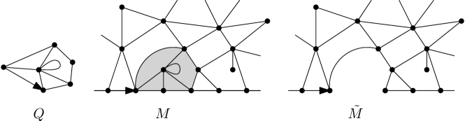
Figure 2: Left: A finite map $Q$. Centre: part of a map $M$ containing $Q$ with $2$ edges along the boundary. Right: the resulting map $\tilde{M}$. The domain Markov property states that $\tilde{M}$ has the same law as $M$.

We now make this precise. Let $Q$ be a finite map in an $m$-gon for some finite $m$, and suppose the boundary of $Q$ is simple (i.e. is a simple cycle in the graph of $Q$), and let $0<k<m$ be some integer. Define the event $A_{Q,k}\subset\mathcal{H}$ that the map $M$ contains a sub-map which is isomorphic to $Q$, and which contains the $k$ boundary edges immediately to the right of the root edge of $M$, and no other boundary edges or vertices. Moreover, we require that the root edge of $Q$ corresponds to the edge immediately to the right of the root of $M$. On this event, we can think of $Q$ as being a subset of $M$, and define the map $\tilde{M}=M\setminus Q$, with the understanding that we keep vertices and edges in $Q$ if they are part of a face not in $Q$ (see Figure 2). Note that $\tilde{M}$ is again a half-planar infinite map.

Definition 1.1.

A probability measure $\mu$ on $\mathcal{H}$ is said to be domain Markov, if for any finite map $Q$ and $k$ as above, the law of $\tilde{M}$ constructed from a sample $M$ of $\mu$ conditioned on the event $A_{Q,k}$ is equal to $\mu$.

Note that for translation invariant measures, the choice of the $k$ edges to the right of the root edge is rather arbitrary: any $k$ edges will result in $\tilde{M}$ with the same law. Similarly, we can re-root $\tilde{M}$ at any other deterministically chosen edge. Thus it is also possible to consider $k$ edges that include the root edge, and mark a new edge as the root of $\tilde{M}$.

This definition is a relatively restrictive form of the domain Markov property. There are several other natural definitions, which we shall discuss below. While some of these definitions are superficially stronger, it turns out that several of them are equivalent to Definition 1.1.

1.2 Main results

Our main result is a complete classification and description of all probability measures on $\mathcal{H}^{\prime}_{p}$ which are translation invariant and have the domain Markov property.

Theorem 1.2.

Fix $p\geq 3$. The set of domain Markov, translation invariant probability measures on $\mathcal{H}^{\prime}_{p}$ forms a one parameter family $\{\mathbb{H}^{(p)}_{\alpha}\}$ with $\alpha\in\mathcal{I}_{p}\subset[0,1)$. The parameter $\alpha$ is the measure of the event that the $p$-gon incident to any fixed boundary edge is also incident to $p-2$ internal vertices.

Moreover, for $p=3$, $\mathcal{I}_{3}=[0,1)$, and for $p>3$ we have $(\alpha_{0}(p),1)\subset\mathcal{I}_{p}$ for some $\alpha_{0}(p)<1$.

We believe that $\mathcal{I}_{p}=[0,1)$ for all $p$ although we have been able to prove this fact only for $p=3$. We emphasise here that our approach would work for any $p$ provided we have certain enumeration results. See Section 3.5 for more on this.

We shall normally omit the superscript $(p)$, as $p$ is thought of as any fixed integer. The measures $\mathbb{H}^{(p)}_{\alpha}$ are all mixing with respect to the translation $\theta$ and in particular are ergodic. This actually follows from a much more general proposition which is well known among experts for the standard half planar random maps, but we could not locate a reference. We include it here for future reference.

Proposition 1.3.

Let $\mu$ be domain Markov and translation invariant on $\mathcal{H}$. Then the translation operator is mixing on $(\mathcal{H},\mu)$, and in particular is ergodic.

Proof.

Let $Q,Q^{\prime}$ and $A_{Q,k},A_{Q^{\prime},k^{\prime}}$ be as in Definition 1.1. Since events of the form $A_{Q,k}$ are simple events in the local topology (see Section 2.2 for more), it suffices to prove that

$$\mu(A_{Q,k}\cap\theta^{n}(A_{Q^{\prime},k^{\prime}}))\to\mu(A_{Q,k})\mu(A_{Q^{\prime},k^{\prime}})$$

as $n\to\infty$ where $\theta^{n}$ is the $n$-fold composition of the operator $\theta$. However, since on $A_{Q,k}$ the remaining map $\widetilde{M}=M\setminus Q$ has the same law as $M$, and since $\theta^{n}(A_{Q^{\prime},k^{\prime}})$ is just $\theta^{n^{\prime}}(A_{Q^{\prime},k^{\prime}})$ in $\widetilde{M}$, for some $n^{\prime}$, we find from the domain Markov property that for large enough integer $n$, the equality $\mu(A_{Q,k}\cap\theta^{n}(A_{Q^{\prime},k^{\prime}}))=\mu(A_{Q,k})\mu(A_{Q^{\prime},k^{\prime}})$ holds. ∎

An application of Proposition 1.3 shows that the measures in the set $\{\mathbb{H}^{(p)}_{\alpha}:\alpha\in\mathcal{I}\}$ are all singular with respect to each other. This is because the density of the edges on the boundary for which the $p$-gon containing it is incident to $p-2$ internal vertices is precisely $\alpha$ by translation invariance. Note that the domain Markov property is not preserved by convex combinations of measures, so the measures $\mathbb{H}_{\alpha}$ are not merely the extremal points in the set of domain Markov measures.

Note also that the case $\alpha=1$ is excluded. It is possible to take a limit $\alpha\to 1$, and in a suitable topology we even get a deterministic map. However, this map is not locally finite and so this can only hold in a topology strictly weaker than the local topology on rooted graphs. Indeed, this map is the plane dual of a tree with one vertex of infinite degree (corresponding to the external face) and all other vertices of degree $p$. As this case is rather degenerate we shall not go into any further details.

In the case of triangulations we get a more explicit description of the measures $\mathbb{H}^{(3)}_{\alpha}$, which we use in a future paper [6] to analyze their geometry. This can be done more easily for triangulations because of readily available and very explicit enumeration results. We believe deriving similar explicit descriptions for other $p$-angulations, at least for even $p$ is possible with a more careful treatment of the associated generating functions, but leave this for future work. This deserves some comment, since in most works on planar maps the case of quadrangulations $q=4$ yields the most elegant enumerative results. The reason the present work differs is the aforementioned necessity of working with simple maps. In the case of triangulations this precludes having any self loops, but any triangle with no self loop is simple, so there is no other requirement. For any larger $p$ (including $4$), the simplicity does impose further conditions. For example, a quadrangulation may contain a face consisting of two double edges.

We remark also that forbidding multiple edges in maps does not lead to any interesting domain Markov measures. The reason is that in a finite map $Q$ it is possible that there exists an edge between any two boundary vertices. Thus on the event $A_{Q,k}$, it is impossible that $\tilde{M}$ contains any edge between boundary edges. This reduces one to the degenerate case of $\alpha=1$, which is not a locally finite graph and hence excluded.

Our second main result is concerned with limits of uniform measures on finite maps. Let $\mu_{m,n}$ be the uniform measure on all simple triangulations of an $m$-gon containing $n$ internal (non-boundary) vertices (or equivalently, $2n+m-2$ faces, excluding the external face). Recall we assume that the root edge is one of the boundary edges. The limits as $n\to\infty$ of $\mu_{m,n}$ w.r.t. the local topology on rooted graphs (formally defined in Section 2.2) have been studied in [7], and lead to the well-known UIPT. Similar limits exist for other classes of planar maps, see e.g. [21] for the case of quadrangulations. It is possible to take a second limit as $m\to\infty$, and the result is the half-plane UIPT measure (see also [17] for the case of quadrangulations). A second motivation for the present work is to identify other possible accumulation points of $\mu_{m,n}$. These measures would be the limits as $m,n\to\infty$ jointly with a suitable relation between them.

Theorem 1.4.

Consider sequences of non-negative integers $m_{l}$ and $n_{l}$ such that $m_{l},n_{l}\to\infty$, and $m_{l}/n_{l}\to a$ for some $a\in[0,\infty]$. Then $\mu_{m_{l},n_{l}}$ converges weakly to $\mathbb{H}^{(3)}_{\alpha}$ where $\alpha=\frac{2}{2a+3}$.

The main thing to note is that the limiting measure does not depend on the sequences $\{m_{l},n_{l}\}$, except through the limit of $m_{l}/n_{l}$. A special case is the measure $\mathbb{H}_{2/3}$ which correspond to the half-planar UIPT measure. Note that in this case, $a=0$, that is the number of internal vertices grows faster than the boundary. Note that the only requirement to get this limit is $m_{l}=o(n_{l})$. This extends the definition of the half-planar UIPT, where we first took the limit as $n_{l}\to\infty$ and only then let $m_{l}\to\infty$.

The other extreme case $\alpha=0$ (or $a=\infty$) is also of special interest. To look into this case it is useful to consider the dual map. Recall that the dual map $M^{*}$ of a planar map $M$ is the map with a vertex corresponding to each face of $M$ and an edge joining two neighbouring faces (that is faces which share at least an edge), or more precisely a dual edge crossing every edge of $M$. Note that for a half-planar map $M$, there will be a vertex of infinite degree corresponding to the face of infinite degree. All other vertices shall have a finite degree ($p$ in the case of $p$-angulations). To fit into the setting of locally finite planar maps, we can simply delete this one vertex, though a nicer modification is to break it up instead into infinitely many vertices of degree $1$, so that the degrees of all other vertices are not changed. For half planar triangulations this gives a locally finite map which is $3$-regular except for an infinite set of degree $1$ vertices, each of which corresponds to a boundary edge. We can similarly define the duals of triangulations of an $m-$gon, where each vertex is of degree $3$ except for $m$ degree $1$ vertices.

For a triangulation of an $m-$gon with no internal vertices ($n=0$), the dual is a $3$ regular tree with $m$ leaves. Let $T$ be the critical Galton-Watson tree where a vertex has $0$ or $2$ offspring with probability $1/2$ each. We add a leaf to the root vertex, so that all internal vertices of $T$ have degree $3$. Then the law of $M^{*}$ under $\mu_{m,0}$ is exactly $T$ conditioned to have $m$ leaves. This measure has a weak limit known as the critical Galton-Watson tree conditioned to survive. This is the law of the dual map $M^{*}$ under $\mathbb{H}_{0}$. Observe that in $\mathbb{H}_{0}$, $\alpha=0$, hence the probability that the triangle incident to any boundary edge has the third vertex also on the boundary is $1$. As before, note that the only condition on $m_{l},n_{l}$ in Theorem 1.4 to get this limiting measure is that $n_{l}=o(m_{l})$. For $p>3$ the measure $\mathbb{H}^{(p)}_{0}$ has a similar description using trees with $p-1$ or $0$ offspring.

Note that Theorem 1.4 gives finite approximations of $\mathbb{H}_{\alpha}$ for $\alpha\in[0,2/3]$, so it is natural to ask for finite approximations to $\mathbb{H}_{\alpha}$ for $\alpha\in(2/3,1)$? In this regime, the maps behave differently than those in the regime $\alpha<2/3$ or $\alpha=2/3$. Maps with law $\mathbb{H}_{\alpha}^{(3)}$ are hyperbolic in nature, and for example have exponential growth (we elaborate on the difference in Section 3.3 and investigate this further in [6]). Benjamini and Curien conjectured (see [10]) that planar quadrangulations exhibiting similar properties can be obtained as distributional limits of finite quadrangulations whose genus grows linearly in the number of faces (for definitions of maps on general surfaces, see for example [22]). The intuition behind such a conjecture is that in higher genus triangulations, the average degree is higher than $6$, which gives rise to negative curvature in the limiting maps, provided the distributional limit is planar. Along similar lines, we think that triangulations on a surface of linear genus size with a boundary whose size also grows to infinity are candidates for finite approximations to $\mathbb{H}_{\alpha}$ for $\alpha\in(2/3,1)$. As indicated in Section 4.1, a similar phase transition is expected for $p$-angulations as well. Thus, we expect a similar conjecture about finite approximation to hold for any $p$, and not only triangulations.

1.3 Other approaches to the domain Markov property

In this section we discuss alternative possible definitions of the domain Markov property, and their relation to Definition 1.1. The common theme is that a map $M$ is conditioned to contain a certain finite sub-map $Q$, connected to the boundary at specified locations. We then remove $Q$ to get a new map $\tilde{M}$. The difficulty arises because it is possible in general for $\tilde{M}$ to contain several connected components. See Figure 3 for some ways in which this could happen, even when the map $Q$ consists of a single face.

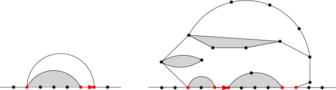
Figure 3: Possibilities when removing a sub-map $Q$ connected to the boundary. The red part is $C_{M}$ which is identified with $C_{Q}$. Left: $Q$ consists of a single triangle. Right: $Q$ consists of two faces in a general map. The shaded areas are the holes — finite components of the complement of $Q$.

To make this precise, we first introduce some topological notions. A sub-map of a planar map $M$ is a subset of the faces of $M$ along with the edges and vertices contained in them. We shall consider a map as a subset of the sphere on which it is embedded.

Definition 1.5.

A sub-map of a planar map is said to be connected if it is connected as subset of the sphere. A connected sub-map $E$ of a half planar map $M$ is said to be simply connected if its union with the external face of $M$ is a simply connected set in the sphere.

Let $Q$ denote a finite planar map, and let some (but at least one) of its faces be marked as external, and the rest as internal. We assume that the internal faces of $Q$ are a connected set in the dual graph $Q^{*}$. One of the external faces of $Q$ is singled out, and a non-empty subset $C_{Q}$ containing at least one edge of the boundary of that external face is marked (in place of the $k$ edges we had before). Note that $C_{Q}$ need not be a single segment now. Fix also along the boundary of $M$ a set $C_{M}$ of the same size as $C_{Q}$, consisting of segments of the same length as those of $C_{Q}$ and in the same order. We consider the event

$$A_{Q}=\{Q\subset M,\partial M\cap\partial Q=C_{M}\},$$

that $Q$ is a sub-map of $M$, with $C_{Q}$ corresponding to $C_{M}$. Figure 3 shows an example of this where $Q$ has a single face.

On the event $A_{Q}$, the complement $M\setminus Q$ consists of one component with infinite boundary in the special external face of $Q$, and a number of components with finite boundary, one in each additional external face of $Q$. Let us refer to the components with finite boundary sizes as holes. Note that because $M$ is assumed to be one-ended, the component with infinite boundary size, which is denoted by $\tilde{M}$ is the only infinite component of $M\setminus Q$. All versions of the domain Markov property for a measure $\mu$ state that

conditioned on $A_{Q}$, the infinite component of $M\setminus Q$ has law $\mu$.

However, there are several possible assumptions about the distribution of the components of $M\setminus Q$ in the holes. We list some of these below.

1. No additional information is given about the distribution of the finite components.

2. The finite components are independent of the distribution of the infinite component.

3. The finite components are independent of the distribution of the infinite component and of each other.

4. The law of the finite components depends only on the sizes of their respective boundaries (i.e. two maps $Q$ with holes of the same size give rise to the same joint distribution for the finite components).

It may seem at first that these are all stronger than Definition 1.1, since our definition of the domain Markov property only applies if $Q$ is simply connected, in which case there are no finite components to $M\setminus Q$. This turns out to be misleading. Consider any $Q$ as above, and condition on the finite components of $M\setminus Q$. Together with $Q$ these form some simply connected map $\bar{Q}$ to which we may apply Definition 1.1. Thus for any set of finite maps that fill the holes of $Q$, $\tilde{M}$ has law $\mu$. Since the conditional distribution of $\tilde{M}$ does not depend on our choice for the finite components, the finite components are independent of $\tilde{M}$. Thus options 1 and 2 are both equivalent to Definition 1.1, and the simple-connectivity condition for $Q$ may be dropped.

In the case of $p$-angulations with simple faces, we have a complete classification of domain Markov measures. Along the proof, it will become clear that those in fact also satisfy the stronger forms 3 and 4 of the domain Markov property. This shows that for simple faced maps, every definition of the domain Markov property gives the same set of measures. If we allow non-simple faces, however, then different choices might yield smaller classes. For example, if a non-simple face surrounds two finite components of the map, then under the domain Markov property as defined above, the parts of the map inside these components need not be independent of each other.

1.4 Peeling

Let us briefly describe the concept of peeling which has its roots in the physics literature [28, 1], and was used in the present form in [3]. It is a useful tool for analyzing planar maps, see e.g. applications to percolation and random walks on planar maps in [4, 11, 5]. While there is a version of this in full planar maps, it takes its most elegant form in the half plane case.

Consider a probability measure $\mu$ supported on a subset of $\mathcal{H}$ and consider a sample $M$ from this measure. The peeling process constructs a growing sequence of finite simply-connected sub-maps $(P_{i})$ in $M$ with complements $M_{i}=M\setminus P_{i}$ as follows. (The complement of a sub-map $P$ contains every face not in $P$ and every edge and vertex incident to them.) Initially $P_{0}=\emptyset$ and $M_{0}=M$. Pick an edge $a_{i}$ in the boundary of $M_{i}$. Next, remove from $M_{i}$ the face incident on $a_{i}$, as well as all finite components of the complement. This leaves a single infinite component $M_{i+1}=\tilde{M}_{i}$, and we set $P_{i+1}=M\setminus M_{i+1}$.

If $\mu$ is domain Markov and the choice of $a_{i}$ depends only on $P_{i}$ and an independent source of randomness, but not on $M_{i}$, then the domain Markov property implies by induction that $M_{n}$ has law $\mu$ for every $n$, and moreover, $M_{n}$ is independent of $P_{n}$. We will see that this leads to yet another interesting viewpoint on the domain Markov property.

In general, it need not be the case that $\bigcup P_{i}=M$ (for example, if the distance from the peeling edge $a_{i}$ to the root grows very quickly). However, there are choices of edges $a_{i}$ for which we do have $\bigcup P_{i}=M$ a.s. One way of achieving this is to pick $a_{i}$ to be the edge of $\partial M_{i}$ nearest to the root of $M$ in the sub-map $M_{i}$, taking e.g. the left-most in case of ties. Note that this choice of $a_{i}$ only depends on $P_{i}$ and this strategy will exhaust any locally finite map $M$.

Let $Q_{i}=M_{i-1}\setminus M_{i}=P_{i}\setminus P_{i-1}$ for $i\geq 1$. This is the finite, simply connected map that is removed from $M$ at step $i$. We also mark $Q_{i}$ with information on its intersection with the boundary of $M_{i-1}$ and the peeling edge $a_{i-1}$. This allows us to reconstruct $P_{i}$ by gluing $Q_{1},\dots,Q_{i}$. In this way, the peeling procedure encodes an infinite half planar map by an infinite sequence $(Q_{i})$ of marked finite maps. If the set of possible finite maps is denoted by $\mathcal{S}$, then we have a bijection $\Phi:\mathcal{H}\to\mathcal{S}^{\mathbb{N}}$. It is straightforward to see that this bijection is even a homeomorphism, where $\mathcal{H}$ is endowed with the local topology on rooted graphs (see Section 2.2), and $\mathcal{S}^{\mathbb{N}}$ with the product topology (based on the trivial topology on $\mathcal{S}$).

Now, if $\mu$ is a domain Markov measure on $\mathcal{H}$, then the pull-back measure $\mu^{*}=\mu\circ\Phi^{-1}$ on $\mathcal{S}^{\mathbb{N}}$ is an i.i.d. product measure, since the maps $M_{i}$ all have the same law, and each is independent of all the $Q_{j}$s for $j<i$. However, translation invariance of the original measure does not have a simple description in this encoding.

Organization

In the next section we recall some necessary definitions and results about the local topology and local limits introduced by Benjamini-Schramm, enumeration of planar maps and the peeling procedure. In Section 3 we prove the classification theorem for triangulations (Sections 3.1 and 3.2) and for $p$-angulations (Section 3.5) and also discuss the variation of maps with non-simple faces. In Section 4 we examine limits of uniform measures on finite maps, and prove Theorem 1.4.

2 Preliminaries

2.1 Enumeration of planar maps

In this section we collect some known facts about the number of planar triangulations, and its asymptotic behaviour. Some of our results rely on the generating function for triangulations of a given size. The following combinatorial result may be found in [18], and are derived using the techniques introduced by Tutte [27], or using more recent bijective arguments [24].

Proposition 2.1.

For $n,m\geq 0$, the number of rooted triangulations of a disc with $m+2$ boundary vertices and $n$ internal vertices is

$$\phi_{n,m+2}=\frac{2^{n+1}(2m+1)!(2m+3n)!}{m!^{2}n!(2m+2n+2)!}$$ (2.1)

Note that this formula is for triangulations with multiple edges allowed, but no self-loops (type II in the notations of [7]). The case of $\phi_{0,2}$ requires special attention. A triangulation of a 2-gon must have at least one internal vertex so there are no triangulations with $n=0$, yet the above formula gives $\phi_{0,2}=1$. This is reconciled by the convention that if a $2$-gon has no internal vertices then the two edges are identified, and there are no internal faces.

This makes additional sense for the following reason: Frequently a triangulation of an $m$-gon is of interest not on its own, but as part of a larger triangulation. Typically, it may be used to fill an external face of size $m$ of some other triangulation by gluing it along the boundary. When the external face is a 2-gon, there is a further possibility of filling the hole by gluing the two edges to each other with no additional vertices. Setting $\phi_{0,2}=1$ takes this possibility into account.

Using Stirling’s formula, the asymptotics of $\phi_{n,m}$ as $n\to\infty$ are easily found to be

$$\phi_{n,m}\sim C_{m}n^{-5/2}\left(\frac{27}{2}\right)^{n}.$$

Again, using Stirling’s formula as $m\to\infty$,

$$C_{m+2}=\frac{\sqrt{3}(2m+1)!}{4\sqrt{\pi}m!^{2}}\left(\frac{9}{4}\right)^{m}\sim Cm^{1/2}9^{m}.$$

The power terms $n^{-5/2}$ and $m^{1/2}$ are common to many classes of planar structures. They arise from the common observation that a cycle partitions the plane into two parts (Jordan’s curve Theorem) and that the two parts may generally be triangulated (or for other classes, filled) independently of each other.

We will also sometimes be interested in triangulations of discs where the number of internal vertices is not fixed, but is also random. The following measure is of particular interest:

Definition 2.2.

The Boltzmann distribution on rooted triangulations of an $m$-gon with weight $q\leq\frac{2}{27}$, is the probability measure on the set of finite triangulations with a finite simple boundary that assigns weight $q^{n}/Z_{m}(q)$ to each rooted triangulation of the $m$-gon having $n$ internal vertices, where

$$Z_{m}(q)=\sum_{n}\phi_{n,m}q^{n}.$$

From the asymptotics of $\phi$ as $n\to\infty$ we see that $Z_{m}(q)$ converges for any $q\leq\frac{2}{27}$ and for no larger $q$. The precise value of the partition function will be useful, and we record it here:

Proposition 2.3.

If $q=\theta(1-2\theta)^{2}$ with $\theta\in[0,1/6]$, then

$$Z_{m+2}(q)=\big{(}(1-6\theta)(m+1)+1\big{)}\frac{(2m)!}{m!(m+2)!}\big{(}1-2\theta\big{)}^{-(2m+2)}.$$

In particular, at the critical point $q=2/27$ we have $\theta=1/6$ and $Z$ takes the values

$$Z_{m+2}=Z_{m+2}\left(\frac{2}{27}\right)=\frac{(2m)!}{m!(m+2)!}\left(\frac{9}{4}\right)^{m+1}.$$

The proof can be found as intermediate steps in the derivation of $\phi_{n,m}$ in [18]. The above form may be deduced after a suitable reparametrization of the form given there.

2.2 The local topology on graphs

Let $\mathcal{G}^{*}$ denote the space of all connected, locally finite rooted graphs. Then $\mathcal{G}^{*}$ is endowed with the local topology, where two graphs are close if large balls around their corresponding roots are isomorphic. The local topology is generated by the following metric: for $G,H\in\mathcal{G}^{*}$, we define

$$d(G,H)=\left(R+1\right)^{-1}\qquad\text{where}\qquad R=\sup\{r:B_{r}(G)\cong B_{r}(H)\}.$$

Here $B_{r}$ denotes the ball of radius $r$ around the corresponding roots, and $\cong$ denotes isomorphism of rooted graphs. Note that for the topology it is immaterial whether the root is a vertex or a directed edge. This metric on $\mathcal{G}^{*}$ is non-Archimedian. Finite graphs are isolated points, and infinite graphs are the accumulation points.

The local topology on graphs induces a weak topology on measures on $\mathcal{G}^{*}$. This is closely related to the Benjamini-Schramm limit of a sequence of finite graphs [13], which is the weak limit of the laws of these graphs with a uniformly chosen root vertex.

We consider below the uniform measures $\mu_{m,n}$ on triangulations of an $m$-gon with $n$ internal vertices. Their limits are supported on the closure $\overline{\mathcal{T}}$ of the set of finite triangulations of polygons. This closure includes also infinite triangulations of an $m$-gon, as well as half-plane infinite triangulations. Angel and Schramm [7], considered the measures $\mu_{2,n}$ as $n\rightarrow\infty$ and obtained their weak limit which is known as the uniform infinite planar triangulation (UIPT). We shall consider similar weak limits here.

Following the seminal work of Benjamini and Schramm [13], properties of such limits have attracted much attention in recent years. A recent success is the proof that the UIPT and similar limits are recurrent [19]. Many questions about the UIPT remain open.

3 Classification of half planar maps

3.1 Half planar triangulations

For the sake of clarity, we begin by proving the special case $p=3$ of Theorem 1.2 of half planar triangulations. In the case of triangulations, the number of simple maps and corresponding generating functions are known explicitly, making certain computations simpler. Somewhat surprisingly, the case of quadrangulations is more complex here, and the generating function is not explicitly known. Apart from the lack of explicit formulae, the case of general $p$ presents a number of additional difficulties, and is treated in Section 3.5.

Theorem 3.1.

All translation invariant, domain Markov probability measures on $\mathcal{H}^{\prime}_{3}$ form a one parameter family of measures $\mathbb{H}_{\alpha}$ for $\alpha\in[0,1)$. Moreover, in $\mathbb{H}_{\alpha}$ the probability that the triangle containing any given boundary edge is incident to an internal vertex is $\alpha$.

In what follows, let $\mu$ be a measure supported on $\mathcal{H}^{\prime}_{3}$, that is translation invariant and satisfies the domain Markov property. We shall first define a certain family of events and show that their measures can be calculated by repeatedly using the domain Markov property. Let $T\in\mathcal{H}^{\prime}_{3}$ denote a triangulation with law $\mu$. Let $\alpha$ be the $\mu$-measure of the event that the triangle incident to a fixed boundary edge $e$ is also incident to an interior vertex (call this event $A_{\alpha}$, see Figure 4). The event depends on the boundary edge chosen, but by translation invariance its probability does not depend on the choice of $e$. As stated, our main goal is to show that $\alpha$ fully determines the measure $\mu$.

Figure 4: Basic building blocks for triangulations. Left: the event $A_{\alpha}$. Centre and right: the two events of type $A_{\beta}$.

For $i\geq 1$ define $p^{(r)}_{i,k}$ (resp. $p^{(l)}_{i,k}$) to be the $\mu$-measure of the event that the triangle incident to a fixed boundary edge $e$ of $T$ is also incident to a vertex on the boundary to the right (resp. left) at a distance $i$ along the boundary from the edge $e$ and that this triangle separates $k$ vertices of $T$ that are not on the boundary from infinity. Note that because of translation invariance, these probabilities only depends on $i$ and $k$ and hence we need not specify $e$ in the notation. It is not immediately clear, but we shall see later that $p^{(l)}_{i,k}=p^{(r)}_{i,k}$ (see Corollary 3.4 below). In light of this, we shall later drop the superscript.

The case $i=1$, $k=0$ is of special importance. Since there is no triangulation of a $2$-gon with no internal vertex, if the triangle containing $e$ is incident to a boundary vertex adjacent to $e$, then it must contain also the boundary edge next to $e$. (See also the discussion in Section 2.1.) We call such an event $A_{\beta}$, shown in Figure 4. By translation invariance, we now see that $p^{(r)}_{1,0}=p^{(l)}_{1,0}$. We shall denote $\beta=p^{(r)}_{1,0}=p^{(l)}_{1,0}$.

In what follows, fix $\alpha$ and $\beta$. Of course, not every choice of $\alpha$ and $\beta$ is associated with a domain Markov measure, and so there are some constraints on their values. We compute below these constraints, and derive $\beta$ as an explicit function of $\alpha$ for any $\alpha\in[0,1)$.

Let $Q$ be a finite simply connected triangulation with a simple boundary, and let $B\subsetneq\partial Q$ be a marked, nonempty, connected segment in the boundary $\partial Q$. Fix a segment in $\partial T$ of the same length as $B$, and let $A_{Q}$ be the event that $Q$ is isomorphic to a sub-triangulation of $T\in\mathcal{H}^{\prime}_{3}$ with $B$ being mapped to the fixed segment in $\partial T$, and no other vertex of $Q$ being mapped to $\partial T$. Let $F(Q)$ be the number of faces of $Q$, $V(Q)$ the number of vertices of $Q$ (including those in $\partial Q$), and $V(B)$ the number of vertices in $B$, including the endpoints.

Lemma 3.2.

Let $\mu$ be a translation invariant domain Markov measure on $\mathcal{H}_{3}^{\prime}$. Then for an event $A_{Q}$ as above we have

$$\mu(A_{Q})=\alpha^{V(Q)-V(B)}\beta^{F(Q)-V(Q)+V(B)}$$ (3.1)

Furthermore, if a measure $\mu$ satisfies (3.1) for any such $Q$, then $\mu$ is translation invariant and domain Markov.

Remark 3.3.

$V(Q)-V(B)$ is the number of vertices of $Q$ not on the boundary of $T$. This shows that the probability of the event $A_{Q}$ depends only on the number of vertices not on the boundary of $T$ and the number of faces of $Q$, but nothing else.

The proof of Lemma 3.2 is based on the idea that the events $A_{\alpha}$ and $A_{\beta}$ form basic “building blocks” for triangulations. More precisely, there exists some ordering of the faces of $Q$ such that if we reveal triangles of $Q$ in that order and use the domain Markov property, we only encounter events of type $A_{\alpha}$, $A_{\beta}$. Moreover, in any such ordering the number of times we encounter the events $A_{\alpha}$ and $A_{\beta}$ are the same as for any other ordering. Also observe that, for every event of type $A_{\alpha}$ encountered, we add a new vertex while for every event of type $A_{\beta}$ encountered, we add a new face. Thus the exponent of $A_{\alpha}$ counts the number of “new” vertices added while the exponent of $A_{\beta}$ counts the number of “remaining” faces.

Proof of Lemma 3.2.

We prove (3.1) by induction on $F(Q)$: the number of faces of $Q$. If $F(Q)=1$, then $Q$ is a single triangle, and $B$ contains either one edge or two adjacent edges. If it has one edge, then the triangle incident to it must have the third vertex not on the boundary of $T$. By definition, in this case $\mu(A_{Q})=\alpha$ and we are done since $V(Q)=3$ and $V(B)=2$. Similarly, if $B$ contains two edges, then $V(B)=3$ and $A_{Q}$ is just the event $A_{\beta}$, with probability $\beta$, consistent with (3.1).

Next, call the vertices of $Q$ that are not in $B$ new vertices. Suppose $F(Q)=n$, and that we have proved the lemma for all $Q^{\prime}$ with $F(Q)<n$. Pick an edge $e_{0}$ from $B$ (there exists one by hypothesis), and let $\Gamma$ be the face of $Q$ incident to this edge. There are three options, depending on where the third vertex of $\Gamma$ lies in $Q$ (see Figure 5):

• the third vertex of $\Gamma$ is internal in $Q$,

• the third vertex of $\Gamma$ is in $\partial Q\setminus B$,

• the third vertex of $\Gamma$ is in $B$.

We treat each of these cases separately.

Figure 5: Cases in the inductive step in the proof of Lemma 3.2.

In the first case, we have that $Q^{\prime}=Q-\Gamma$ is also a simply connected triangulation, if we let $B^{\prime}$ include the remaining edges from $B$ as well as the two new edges from $\Gamma$, we can apply the induction hypothesis to $Q^{\prime}$. By the domain Markov property, we have that

$$\mu(A_{Q})=\mu(A_{\Gamma})\mu(A_{Q}|A_{\Gamma})=\alpha\mu(A_{Q^{\prime}}).$$

This implies the claimed identity for $Q$, since $Q^{\prime}$ has one less face and one less new vertex than $Q$.

In the case where the third vertex of $\Gamma$ is in $\partial Q\setminus B$, we have a decomposition $Q=\Gamma\cup Q_{1}\cup Q_{2}$, where $Q_{1}$ and $Q_{2}$ are the two connected components of $Q\setminus\Gamma$ (see Figure 5). We define $B_{i}$, to contain the edges of $B$ in $Q_{i}$, and one edge of $\Gamma$ that is in $Q_{i}$. We have that $F(Q)=F(Q_{1})+F(Q_{2})+1$, and that the new vertices in $Q_{1}$ and $Q_{2}$ except for the third vertex of $F(Q)$ together are the new vertices of $Q$. By the domain Markov property, conditioned on $A_{\Gamma}$, the inclusion of $Q_{1}$ and of $Q_{2}$ in $T$ are independent events with corresponding probabilities $\mu(A_{Q_{i}})$. Thus

$$\mu(A_{Q})=\alpha\mu(A_{Q_{1}}|A_{\Gamma})\mu(A_{Q_{2}}|A_{\Gamma})=\alpha\mu(A_{Q_{1}})\mu(A_{Q_{2}})=\alpha^{V(Q)-V(B)}\beta^{F(Q)-V(Q)+V(B)},$$

as claimed.

Finally, consider the case that the third vertex of $\Gamma$ is in $B$. As in the previous case, we have a decomposition $Q=\Gamma\cup Q_{1}\cup Q_{2}$, where $Q_{1}$ is the triangulation separated from infinity by $\Gamma$, and $Q_{2}$ is the part adjacent to the rest of $T$ (see Figure 5.) We let $B_{1}$ consist of the edges of $B$ in $Q_{1}$ and let $B_{2}$ be the edges of $B$ in $Q_{2}$ with the additional edge of $\Gamma$. We then have

$$\mu(A_{Q})=\mu(A_{Q_{1}})\mu(A_{Q_{1}\cup\Gamma}|A_{Q_{1}})\mu(A_{Q}|A_{Q_{1}\cup\Gamma}).$$

By the induction hypothesis, the first term is $\alpha^{V(Q_{1})-V(B_{1})}\beta^{F(Q_{1})-V(Q_{1})+V(B_{1})}$. By the domain Markov property, the second term is just $\beta$. Similarly, the third term is $\alpha^{V(Q_{2})-V(B_{2})}\beta^{F(Q_{2})-V(Q_{2})+V(B_{2})}$. As before we have that $F(Q)=F(Q_{1})+F(Q_{2})+1$, and this time $V(Q)-V(B)=(V(Q_{1})-V(B_{1}))+(V(Q_{2})-V(B_{2}))$, since the new vertices of $Q$ are the new vertices of $Q_{1}$ together with the new vertices of $Q_{2}$. The claim again follows.

Note that in the last case it is possible that $Q_{1}$ is empty, in which case $\Gamma$ contains two edges from $\partial Q$. All formulae above hold in this case with no change.

For the converse, note first that since the events $A_{Q}$ are a basis for the local topology on rooted graphs, they uniquely determine the measure $\mu$. Moreover, the measure of the events of the form $A_{Q}$ do not depend on the location of the root and so $\mu$ is translation invariant. Now observe from Remark 3.3 that the measure of any event of the form $A_{Q}$ only depends on the number of new vertices and the number of faces in $Q$. Now suppose we remove any simple connected sub-map $Q_{1}$ from $Q$. Then the union of new vertices in $Q_{1}$ and $Q\setminus Q_{1}$ gives the new vertices of $Q$. Also clearly, the union of the faces of $Q_{1}$ and $Q\setminus Q_{1}$ gives the faces of $Q$. Hence it follows that $\mu(A_{Q}|A_{Q_{1}})=\mu(A_{Q\setminus Q_{1}})$, and thus $\mu$ is domain Markov. ∎

Corollary 3.4.

For any $i,k$ we have

$$p^{(r)}_{i,k}=p^{(l)}_{i,k}=\phi_{k,i+1}\alpha^{k}\beta^{i+k}$$ (3.2)

Proof.

This is immediate because the event with probability $p_{i,k}$ is a union of $\phi_{k,i+1}$ disjoint events of the form $A_{Q}$, corresponding to all possible triangulations of an $i+1$-gon with $k$ internal vertices. A triangulation contributing to $\phi_{k,i+1}$ has $k$ internal vertices by the Euler characteristic formula, $2k+i-1$ faces. The triangle that separates it from the rest of the map is responsible for the extra factor of $\beta$. ∎

Since the probability of any finite event in $\mathcal{H}^{\prime}_{3}$ can be computed in terms of the peeling probabilities $p_{i,k}$’s, we see that for any given $\alpha$ and $\beta$ we have at most a unique measure $\mu$ supported on $\mathcal{H}^{\prime}_{3}$ which is translation invariant and satisfies the domain Markov property. The next step is to reduce the number of parameters to one, thereby proving the first part of Theorem 3.1. This is done in the following lemma.

Lemma 3.5.

Let $\mu$ be a domain Markov, translation invariant measure on $\mathcal{H}^{\prime}_{3}$, and let $\alpha$,$\beta$ be as above. Then

$$\beta=\begin{cases}\frac{1}{16}(2-\alpha)^{2}&\alpha\leq 2/3,\\ \frac{1}{2}\alpha(1-\alpha)&\alpha\geq 2/3.\end{cases}$$

Proof.

The key is that since the face incident to the root edge is either of type $\alpha$, or of the type with probability $p_{i,k}$ for some $i,k$, (with $i=1,k=0$ corresponding to type $\beta$) we have the identity

$$\alpha+\sum_{i\geq 1}\sum_{k\geq 0}\left(p^{(r)}_{i,k}+p^{(l)}_{i,k}\right)=1.$$

In light of Corollary 3.4 we may write this as

$$1=\alpha+2\sum_{i}\beta^{i}\sum_{k}\phi_{k,i+1}(\alpha\beta)^{k}=\alpha+2\sum_{i}\beta^{i}Z_{i+1}(\alpha\beta).$$

From Proposition 2.3 we see that the sum above converges if and only if $\alpha\beta\leq\frac{2}{27}$. In that case, there is a $\theta\in[0,1/6]$ with $\alpha\beta=\theta(1-2\theta)^{2}$. Using the generating function for $\phi$ (see e.g. [18]) and simplifying gives the explicit identity

$$(2\theta+\alpha-1)\sqrt{1-\frac{4\theta}{\alpha}}=0.$$ (3.3)

Thus $\theta\in\{\frac{1-\alpha}{2},\frac{\alpha}{4}\}$. Of these, only one solution satisfies $\theta\in[0,1/6]$ for any value of $\alpha$. If $\alpha\leq 2/3$, then we must have $\theta=\alpha/4$ which yields

$$\beta=\frac{1}{4}\left(1-\frac{\alpha}{2}\right)^{2}=\frac{1}{16}(2-\alpha)^{2}$$

If $\alpha\geq 2/3$ one can see from (3.3) that the solution satisfying $\theta\in[0,1/6]$ is $\theta=(1-\alpha)/2$ which in turn gives

$$\beta=\frac{\alpha(1-\alpha)}{2}.\qed$$

3.2 Existence

As we have determined $\beta$ in terms of $\alpha$, and since Lemma 3.2 gives all other probabilities $p_{i,k}$ in terms of $\alpha$ and $\beta$, we have at this point proved uniqueness of the translation invariant domain Markov measure with a given $\alpha<1$. However we still need to prove that such a measure exists. We proceed now to give a construction for these measures, via a version of the peeling procedure (see Section 1.4). For $\alpha\leq 2/3$, we shall see with Theorem 1.4 that the measures $\mathbb{H}_{\alpha}$ can also be constructed as local limits of uniform measures on finite triangulations.

In light of Lemma 3.2, all we need is to construct a probability measure $\mu$ such that the measure of the events of the form $A_{Q}$ (as defined in Lemma 3.2) is given by (3.1).

If we reveal a face incident to any fixed edge in a half planar triangulation along with all the finite components of its complement, then the revealed faces form some sub-map $Q$. The events $A_{Q}$ for such $Q$ are disjoint, and form a set we denote by $\mathcal{A}$. If we choose $\alpha$ and $\beta$ according to Lemma 3.5, then the prescribed measure of the union of the events in $\mathcal{A}$ is $1$.

Let $\alpha$ and let $\beta$ be given by Lemma 3.5. We construct a distribution $\mu_{r}$ on the hull of the ball of radius $r$ in the triangulation (which consists of all faces with a corner at distance less than $r$ from the root, and with the holes added to make the hull).

Repeatedly pick an edge on the boundary which has at least an endpoint at a distance strictly less than $r$ from the root edge in the map revealed so far. Note that as more faces are added to the map, distances may become smaller, but not larger. Reveal the face incident to the chosen edge and all the finite components of its complement. Given $\alpha$ and $\beta$ we pick which event in $\mathcal{A}$ occurs by (3.1), independently for different steps. We continue the process as long as any vertex on the exposed boundary is at distance less than $r$ from the root. Note that this is possible since the revealed triangulation is always simply connected with at least one vertex on the boundary, the complement must be the upper half plane.

Proposition 3.6.

The above described process a.s. ends after finitely many steps. The law of the resulting map does not depend on the order in which we choose the edges.

Proof.

We first show that the process terminates for some order of exploration. The following argument for termination is essentially taken from [3]. Assume that at each step we pick a boundary vertex at minimal distance (say, $k$) from the root (w.r.t. the revealed part of the map), and explore along an edge containing that vertex. At any step with probability $\beta>0$ we add a triangle such that the vertex is no longer on the boundary. Any new revealed vertex must have distance at least $k+1$ from the root. Moreover, any vertex that before the exploration step had distance greater than $k$ to the root, still has distance greater than $k$, since the shortest path to any vertex must first exit the part of the map revealed before the exploration step. Thus the number of vertices at distance $k$ to the root cannot increase, and has probability $\beta>0$ of decreasing at each step. Thus a.s. after a finite number of steps all vertices at distance $k$ are removed from the boundary. Once we reach distance $r$, we are done.

The probability of getting any possible map $T$ is a monomial in $\alpha$ and $\beta$, and is the same regardless of the order in which the exploration takes place (with one $\alpha$ for each non-boundary vertex of the map, and a $\beta$ term for the difference between faces and vertices). It remains to show that the process terminates for any other order of exploration. For some order of exploration, let $\nu_{i}(T)$ be the probability that the process terminated after at most $i$ steps and revealed $T$ as the ball of radius $r$. For $i$ large enough (larger than the number of faces in $T$) we have that $\nu_{i}(T)=\mu_{r}(T)$. Summing over $T$ and taking the limit as $i\to\infty$, Fatou’s lemma implies that $\lim_{i}\sum_{T}\nu_{i}(T)\geq\sum\mu_{r}(T)$. However, the last sum must equal 1, since for some order of exploration the process terminates a.s. ∎

It is clear from Proposition 3.6 that $\mu_{r}$ is a well-defined probability measure. Since we can first create the hull of radius $r$ and then go on to create the hull of radius $r+1$, $(\mu_{r})$ forms a consistent sequence of measures. By Kolmogorov’s extension Theorem, $(\mu_{r})_{r\in\mathbb{N}}$ can be extended to a measure $\mathbb{H}_{\alpha}$ on $\mathcal{H}^{\prime}_{3}$. Also, we have the following characterization of $\mathbb{H}_{\alpha}$ for any simple event of the form $A_{Q}$ as defined in Lemma 3.2.

Lemma 3.7.

For any $A_{Q}$ and $B$ as defined in Lemma 3.2,

$$\mathbb{H}_{\alpha}(A_{Q})=\alpha^{V(Q)-V(B)}\beta^{F(Q)-V(Q)+V(B)}$$ (3.4)

We alert the reader that such a characterization is not obvious from the fact that the events of the form $\{\overline{B_{r}}=T\}$ have the $\mathbb{H}_{\alpha}$ measure exactly as asserted by Lemma 3.7 where $\overline{B_{r}}$ denotes the hull of the ball of radius $r$ around the root vertex. Any finite event like $A_{Q}$ can be written in terms of the measures of $\mathbb{H}_{\alpha}(\overline{B_{r}}=T)$ for different $T\in\mathcal{T}$ by appropriate summation. However it is not clear a priori that the result will be as given by (3.4).

Proof of Lemma 3.7.

Since $Q$ is finite, there exists a large enough $r$ such that $Q$ is a subset of $\overline{B_{r}}$. Now we claim that $\mu_{r}(A_{Q})$ is given by the right hand side of (3.4). This is because crucially, $\mu_{r}$ is independent of the choice of the sequence of edges, and hence we can reveal the faces of $Q$ first and then the rest of $\overline{B_{r}}$. However the measure of such an event is given by the right hand side of (3.4) by the same logic as Proposition 3.6. Now the lemma is proved because $\mathbb{H}_{\alpha}(A_{Q})=\mu_{r}(A_{Q})$ since $\mathbb{H}_{\alpha}$ is an extension of $\mu_{r}$. ∎

We now have all the ingredients for the proof of Theorem 3.1.

Proof of Theorem 3.1.

We have the measures $\mathbb{H}_{\alpha}$ constructed above which are translation invariant and domain Markov (from the second part of Lemma 3.2). If $\mu$ is a translation invariant domain Markov measure, then by Lemmas 3.2, 3.5 and 3.7, $\mu$ agrees with $\mathbb{H}_{\alpha}$ on every event of the form $A_{Q}$, and thus $\mu=\mathbb{H}_{\alpha}$ for some $\alpha$. ∎

3.3 The phase transition

In the case of triangulations, we call the measures $\mathbb{H}_{\alpha}$ subcritical, critical and supercritical when $\alpha<\frac{2}{3}$, $\alpha=\frac{2}{3}$, and $\alpha>\frac{2}{3}$ respectively. We summarize here for future reference the peeling probabilities $p_{i,k}$ and $p_{i}=2\sum_{k\geq 0}p_{i,k}$ for every $\alpha\in[0,1)$. Recall that $\theta$ is defined by $\alpha\beta=\theta(1-2\theta)^{2}$ and $\theta\in[0,\frac{1}{6}]$.

Critical case: $\alpha=\frac{2}{3}$

This case is the well-known half plane UIPT (see [3], Section 1.) Here $\beta=\frac{1}{9}$ and $\theta=\frac{1}{6}$. The two possible values of $\theta$ coincide at $\frac{1}{6}$ and hence $\beta=\frac{1}{9}$. Using Corollaries 3.4 and 2.3, we recover the probabilities

$$\begin{split}p_{i,k}&=\phi_{k,i+1}\left(\frac{1}{9}\right)^{i}\left(\frac{2}{27}\right)^{k}\\ p_{i}&=\frac{2}{4^{i}}\frac{(2i-2)!}{(i-1)!(i+1)!}\end{split}$$ (3.5)

Note that in $\mathbb{H}_{2/3}$ we have the asymptotics $p_{i}\sim ci^{-5/2}$ for some $c>0$.

Sub-critical case: $\alpha<\frac{2}{3}$

Here $\theta=\alpha/4$ and hence $\beta=\frac{(2-\alpha)^{2}}{16}$. Using Corollary 3.4 and Proposition 2.3, we get

$$\begin{split}p_{i,k}&=\phi_{k,i+1}\left(\frac{2-\alpha}{4}\right)^{2i}\left(\frac{\alpha}{4}\left(1-\frac{\alpha}{2}\right)^{2}\right)^{k}\\ p_{i}&=\frac{2}{4^{i}}\frac{(2i-2)!}{(i-1)!(i+1)!}\cdot\left(\left(1-\frac{3\alpha}{2}\right)i+1\right)\end{split}$$ (3.6)

As before, we get the asymptotics $p_{i}\sim ci^{-3/2}$ for some $c=c(\alpha)>0$. Note that $p_{i}$ is closely related to a linearly biased version of $p_{i}$ for the critical case.

Super-critical case: $\alpha>2/3$

Here $\theta=\frac{1-\alpha}{2}$ and hence $\beta=\frac{\alpha(1-\alpha)}{2}$. Using Corollary 3.4 and Proposition 2.3, we get

$$\begin{split}p_{i,k}&=\phi_{k,i+1}\alpha^{i+2k}\left(\frac{1-\alpha}{2}\right)^{i+k}\\ p_{i}&=\frac{2}{4^{i}}\frac{(2i-2)!}{(i-1)!(i+1)!}\cdot\left(\frac{2}{\alpha}-2\right)^{i}((3\alpha-2)i+1)\end{split}$$ (3.7)

Here, the asymptotics of $p_{i}$ are quite different, and $p_{i}$ has an exponential tail: $p_{i}\sim c\gamma^{i}i^{-{3/2}}$ for some $c$ and $\gamma=\frac{2}{\alpha}-2$. The differing asymptotics of the connection probabilities $p_{i}$ indicate very different geometries for these three types of half plane maps. These are almost (though not quite) the probabilities of edges between boundary vertices at distance $i$. We investigate the geometry of the various half-planar maps in a future paper [6].

3.4 Non-simple triangulations

So far, we have only considered one type of maps: triangulations with multiple edges allowed, but no self loops. Forbidding double edges combined with the domain Markov property, leads to a very constrained set of measures. The reason is that a step of type $\alpha$ followed by a step of type $\beta$ can lead to a double edge. If $\mu$ is supported on measures with no multiple edges, this is only possible if $\alpha\beta=0$. As seen from the discussion above, this gives the unique measure $\mathbb{H}_{0}$ which has no internal vertices at all. A similar phenomenon occurs for $p$-angulations for any $p\geq 3$, and we leave the details to the reader.

In contrast, the reason one might wish to forbid self-loops is less clear. We now show that on the one hand, allowing self-loops in a triangulation leads to a very large family of translation invariant measures with the domain Markov property. On the other hand, these measures are all in an essential way very close to one of the $\mathbb{H}_{\alpha}$ measures already encountered. The reason that uniqueness breaks as thoroughly as it does, is that here it is possible for removal of a single face to separate the map into two components, one of which is only connected to the infinite part of the boundary through the removed face. We remark that for triangulations with self loops, the stronger forms of the domain Markov property discussed in Section 1.3 are no longer equivalent to the weaker ones that we use.

Let us construct a large family of domain Markov measures as promised. Our translation invariant measures on triangulations with self-loops are made up of three ingredients. The first is the parameter $\alpha\in[0,1)$ which corresponds to a measure $\mathbb{H}_{\alpha}$ as above. Next, we have a parameter $\gamma\in[0,1)$ which represents the density of self loops. Taking $\gamma=0$ will result in no self-loops and the measure will be simply $\mathbb{H}_{\alpha}$. Finally, we have an arbitrary measure $\nu$ supported on triangulations of the $1$-gon (i.e. finite triangulations whose boundary is a self-loop, possibly with additional self-loops inside). From $\alpha,\gamma$ and $\nu$ we construct a measure denoted $\mathbb{H}_{\alpha,\gamma,\nu}$. More precisely, we describe a construction for a triangulation with law $\mathbb{H}_{\alpha,\gamma,\nu}$.

Given $\alpha$, take a sample triangulation $T$ from $\mathbb{H}_{\alpha}$. For each edge $e$ of $T$, including the boundary edges, take an independent geometric variable $G_{e}$ with $\mathbb{H}_{\alpha,q,\nu}(G_{e}=k)=(1-q)q^{k-1}$. Next, replace the edge $e$ by $G_{e}$ parallel edges, thereby creating $G_{e}-1$ faces which are all $2$-gons. In each of the $2$-gons formed, add a self-loop at one of the two vertices, chosen with equal probability and independently of the choices at all other $2$-gons. This has the effect of splitting the 2-gon into a triangle and a 1-gon. Finally, fill each self-loop created in this way with an independent triangulation with law $\nu$ (see Figure 6).

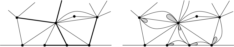
Figure 6: Non-uniqueness for triangulation with self-loops. Starting with a triangulation with simple faces (left), each edge is replaced by a geometric number of parallel edges with a self-loop at one of the two vertices between any pair (greater than 1 at the bold edges). Independent maps with arbitrary distribution are added inside the self-loops (shaded). Note that multiple edges may occur on the left (but not self-loops).

Proposition 3.8.

The measures $\mathbb{H}_{\alpha,q,\nu}$ defined above are translation invariant and satisfy the domain Markov property. For $\alpha>0$, these are all the measures on half planar triangulations with these properties.

Recall that we use $\alpha$ to denote the probability of the event of type $\alpha$ that the triangle incident on any boundary edge also contains an internal vertex. The case of triangulations with $\alpha=0$ is special for reasons that will be clearer after the proof, and is the topic of Proposition 3.9. In that case we shall require another parameter, and another measure $\nu^{\prime}$. This will be the only place where we shall demonstrate domain Markov measures that are not symmetric w.r.t. left-right reflection.

Coming back to the case $\alpha>0$, note that since $\nu$ is arbitrary, the structure of domain Markov triangulations with self-loops is much less restricted than without the self-loops. For example, $\nu$ could have a very heavy tail for the size of the maps, or for the degree of the vertex in the self-loop, which will affect the degree distribution of vertices in the map. However, the measures $\mathbb{H}_{\alpha,q,\nu}$ are closely related to $\mathbb{H}_{\alpha}$, since the procedure described above for generating a sample of $\mathbb{H}_{\alpha,q,\nu}$ from a sample of $\mathbb{H}_{\alpha}$ is reversible. Indeed, if we take a sample from $\mathbb{H}_{\alpha,q,\nu}$ and remove each loop and the triangulation inside it, we are left with a map whose faces are triangles or $2$-gons. If we then glue the edges of each $2$-gon into a single edge, we are left with a simple triangulation. We refer to this operation as taking the 2-connected core of the triangulation, since the dual of the triangulation contains a unique infinite maximal 2-connected component, which is a subdivision of the dual of the triangulation resulting from this operation. Clearly the push-forward of the measures $\mathbb{H}_{\alpha,q,\nu}$ via this operation has law $\mathbb{H}_{\alpha}$. Thus $\mathbb{H}_{\alpha}$ does determine in some ways the large scale structure of $\mathbb{H}_{\alpha,q,\nu}$.

Proof of Proposition 3.8.

Translation invariance is clear as $\mathbb{H}_{\alpha}$ is translation invariant, the variables $G_{e}$ and triangulations in the self-loops do not depend upon the location of the root.

To see that $\mathbb{H}_{\alpha,q,\nu}$ is domain Markov, let $T$ be a half planar triangulation with law $\mathbb{H}_{\alpha,q,\nu}$. Let $\operatorname{core}(\cdot)$ denote the $2$-connected core of a map, and observe that $\operatorname{core}(T)$ is a map with law $\mathbb{H}_{\alpha}$ from which $T$ was constructed. Let $Q$ be a finite simply connected triangulation (which may contain non-simple faces), and let $A_{Q}$ be the event as defined in Lemma 3.2. To establish the domain Markov property for $\mathbb{H}_{\alpha,q,\nu}$, we need to show that conditionally on $A_{Q}$, $\tilde{T}=T\setminus Q$ (as defined in Section 1.1) has the same law as $T$. On the event $A_{Q}$, a corresponding event $A_{\text{core}(Q)}$ that $\operatorname{core}(Q)\subset\operatorname{core}(T)$ also holds. Moreover, on these events, $\operatorname{core}(\tilde{T})=\operatorname{core}(T)\setminus\operatorname{core}(Q)$ has law $\mathbb{H}_{\alpha}$, since $\mathbb{H}_{\alpha}$ is domain Markov. We therefore need to show that to get from $\operatorname{core}(T)\setminus\operatorname{core}(Q)$ to $\tilde{T}$ each edge is replaced by a $\operatorname{Geom}(q)$ number of parallel non-simple triangles with $\nu$-distributed triangulations inside the self-loops. Any edge of $\operatorname{core}(T)\setminus\operatorname{core}(Q)$ is split in $\tilde{T}$ into an independent $\operatorname{Geom}(q)$ number of parallel edges. Indeed, for edges not in $\operatorname{core}(Q)$ this number is the same as in $T$, and for edges in the boundary of $Q$, the number is reduced by those non-simple triangles that are in $Q$, but is still $\operatorname{Geom}(q)$ due to the memory-less property of the geometric variables. The triangulations inside the self-loops are i.i.d. samples of $\nu$, since they are just a subset of the ones in $T$ which are i.i.d. and $\nu$-distributed.

For the second part of the proposition, note first that if $\mu$ is domain Markov, then the push-forward of $\mu$ w.r.t. taking the core is also domain Markov, hence must be $\mathbb{H}_{\alpha}$ for some $\alpha\in[0,1)$ by Theorem 3.1.

Fix an edge along the boundary, let $q$ be the probability that the face containing it is not simple. By the domain Markov property, conditioned on having such a non-simple face and removing it leaves the map unchanged in law, and so this is repeated $\operatorname{Geom}(q)$ times before a simple face is found. Removing all of these faces also does not change the rest of the map, and so this number is independent of the multiplicity at any other edge of the map. Similarly, the triangulation inside the self-loop within each such non simple face is independent of all others, and we may denote its law by $\nu$. Since any edge inside the map may be turned into a boundary edge by removing a suitable finite sub-map, the same holds for all edges.

To see that $\mu=\mathbb{H}_{\alpha,q,\nu}$, it remains to show that the self-loops are equally likely to appear at each end-point of the $2$-gons and are all independent. The independence follows as for the triangulations inside the self-loops. To see that the two end-points are equally likely (and only to this end) we require $\alpha>0$. The configuration shown in Figure 7 demonstrates this. After removing the face on the right, the self-loop is at the right end-point of a $2$-gon on the boundary. Removing the triangle on the left leaves the self-loop on the left end-point, and so the two are equally likely. ∎

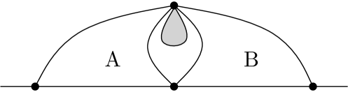
Figure 7: Exploring in different orders shows that self-loops are equally likely to be at each end-point of a $2$-gon. Conditioning on face $A$ and removing it leaves a non-simple face along the boundary with the self-loop at the left vertex. Removing instead face $B$ leaves the self-loop on the right vertex.

As noted above, the case $\alpha=0$ is special. In this case, no boundary edge has its third vertex internal to the triangulation. Note that this is not the same as saying that the triangulation has no internal vertices - they could all be inside self-loops, which are attached to the boundary vertices. The contraction operation described above still necessarily yields a sample $T$ of $\mathbb{H}_{0}$. Similarly, each edge of $T$ must correspond to an independent, geometric number of edges in the full map, and the triangulations inside the corresponding self-loops must be independent.

However, without steps of type $\alpha$ we cannot show that the the two choices for the location of the self-loop in $2$-gons are equally likely. Indeed, since all $2$-gons connect a pair of boundary vertices, it is possible to tell them apart. Adding the self-loop always on the left vertex will not be the same as adding it always on the right. This reasoning leads to a complete characterization also in the case $\alpha=0$. In each $2$-gon the self-loop is on the left vertex with some probability $\gamma\in[0,1]$, and these must be independent of all other $2$-gons. The triangulations inside the self-loops are all independent, but their laws may depend on whether the self-loop is on the left or right vertex in the $2$-gon, so we need to specify two measures $\nu_{L},\nu_{R}$ on triangulations of the $1$-gon. Thus we get the following:

Proposition 3.9.

A domain Markov, translation invariant triangulation with $\alpha=0$ is determined by the intensity of multiple edges $q$, the probability $\gamma\in[0,1]$ that the self-loop is attached to the left vertex in each $2$-gon, and probability measures $\nu_{L},\nu_{R}$ on triangulations of the $1$-gon.

3.5 Simple and general $p$-angulations

Here we prove the general case of Theorem 1.2. The proof is similar to the proof of Theorem 3.1, with some additional complications: There are more than the two types of steps $\alpha$ and $\beta$, and the generating function for simple $p$-angulations is not explicitly known. There are implicit formulae relating it to the generating function for general maps with suitably chosen weights for various face sizes, which are fairly well understood in the case of even $p$. For quadrangulations, even more is known. In [23], the problem of enumerating $2$-connected loopless near $4$-regular planar maps (see [23] for exact definitions) is considered. This is easily equivalent to our problem of enumerating simple faced quadrangulations with a simple boundary. The generating function is computed there in a non-closed form. With careful analysis, this might lead to explicit expressions analogous to the ones we have for the triangulation case at least for the case of quadrangulations. We have not been able to obtain such expressions, and thus our description of the corresponding $\mathbb{H}_{\alpha}$’s still depends on an undetermined parameter $\beta=\beta(\alpha)$. Instead, uniqueness is proved by a softer argument based on monotonicity. The proof of existence used for triangulations goes through with no significant changes, but is now conditional on the existence of a solution to a certain equation.

Proof of Theorem 1.2.

As before, let $\mu$ be a probability measure supported on the set $\mathcal{H}_{p}^{\prime}$ of half planar simple $p$-angulations which is translation invariant and satisfies the domain Markov property. The building blocks for simple $p$-angulations, taking the place of $A_{\alpha}$ and $A_{\beta}$, will be the events where the face incident to the root edge consists of a single contiguous segment from the infinite boundary, together with a simple path in the interior of the map closing the cycle, with the path in any fixed position relative to the root (see Figure 8(a)). The number of internal vertices can be anything from $0$ to $p-2$. Let the $\mu$-measure of such an event with $i$ internal vertices (call the event $A_{i}$) be $\alpha_{i}$ for $i=0,\ldots,p-2$. For example, in the case of $p=3$ we have $\alpha_{1}=\alpha$ and $\alpha_{0}=\beta$. We shall continue to use $\alpha$ for $\alpha_{p-2}$, i.e. the $\mu$-probability that the face on the root edge contains no other boundary vertices. Note that there are several such events of type $A_{i}$, which differ only in the location of the root. However because of translation invariance, each such event has the same probability $\alpha_{i}$. For quadrangulations ($p=4$), there are three possible building blocks, shown in Figure 8(b–d).

Figure 8: Building blocks for quadrangulations and general $p$-angulations. Shown: an event of type $A_{5}$ for $p=9$ and the three building blocks for $p=4$.

We have a generalization of Lemma 3.2, that shows that the measure $\mu$ is determined by $\alpha_{0}\dots,\alpha_{p-2}$, leaving us with $p-1$ degrees of freedom. However, before doing that, let us reduce these to two degrees of freedom. For any $i=1,\dots,p-2$, consider the event $B_{i}$ defined as follows (see e.g. Figure 9):

• The face incident to the root edge has $i-1$ internal vertices and its intersection with the boundary is a contiguous segment of length $p-i+1$ with the leftmost of those vertices being the root.

• The face incident to the edge to the left of the root edge has $i$ internal vertices, its intersection with the boundary is a contiguous segment of length $p-i$, with the root vertex being the right end-point.

• The two faces above share precisely one common edge between them which is also incident to the root vertex.

The probability $\mu(B_{i})$ can be computed by exploring the faces incident to the root edge, and with the edge to its left in the two possible orders. We find that $\alpha_{i-1}^{2}=\alpha_{i}\alpha_{i-2}$, and hence the numbers $\{\alpha_{0},\ldots,\alpha_{p-2}\}$ form a geometric series, leaving two degrees of freedom. In order to simplify subsequent formulae we reparametrize these as follows. Denote

$$\beta^{p-2} =\alpha_{0}, \gamma^{p-2} =\alpha_{p-2}$$

so that the geometric series is given by $\alpha_{i}=\gamma^{i}\beta^{p-2-i}$. This is consistent with the previous definition of $\beta$ in the case $p=3$.

Figure 9: The event $B_{4}$ for $p=6$. Depending on the order of exploration, its probability is found to be $\alpha_{3}^{2}$ or $\alpha_{4}\alpha_{2}$.

Lemma 3.10.

Let $\mu$ be a measure supported on $\mathcal{H}_{p}^{\prime}$ which is translation invariant and domain Markov. Let $Q$ be a finite simply connected simple $p$-angulation and $2\leq k<|\partial Q|$. As before, $A_{Q,k}$ is the event that $Q$ is isomorphic to a sub-map of $M$ with $k$ consecutive vertices being mapped to the boundary of $M$. Then

$$\mu(A_{Q,k})=\alpha_{1}^{V(Q)-k}\alpha_{0}^{F(Q)-V(Q)+k}=\beta^{(p-2)F(Q)-V(Q)+k}\gamma^{V(Q)-k}.$$ (3.8)

Furthermore, if $\mu$ satisfies (3.8) for any such $Q$ and $k$, then $\mu$ is translation invariant and domain Markov.

The proof is almost the same as in the case of triangulations, and we omit some of the repeated details, concentrating only on the differences.

Proof.

We proceed by induction on the number of faces of $Q$. If $Q$ has a single face, then we are looking at one of the events $A_{i}$. Then the face connected to the root sees $i$ new vertices. The measure of such an event is $\alpha_{i}$ which is equal to $\alpha_{0}(\alpha_{1}/\alpha_{0})^{i}$ since $\{\alpha_{0},\ldots,\alpha_{p-2}\}$ form a geometric series. Hence (3.8) holds.

In general, the face $\Gamma$ connected to the root can be connected to the boundary of $Q$ and to the interior of $Q$ in several possible ways. $Q\setminus\Gamma$ has several components some of which are connected to the infinite component of $M\setminus Q$ and some are not. We shall explore the components not connected to the infinite component of $M\setminus Q$ first, then the face $\Gamma$ and finally the rest of the components. Note that in every step of exploration if we encounter an event of type $A_{i}$, we get a factor of $\alpha_{1}^{v}\alpha_{0}^{f-v}$ for the probability, where $v$ is the number of new vertices added and $f$ is the number of new faces added since $\{\alpha_{0},\alpha_{1},\ldots,\alpha_{p}\}$ are in geometric progression. Since the number of new vertices in all the components and $\Gamma$ add up to that of $Q$ and similarly the number of faces in all the components and $\Gamma$ also add up to that of $Q$, this gives the claim. The details are left to the reader. ∎

Returning to the proof of Theorem 1.2, let $Z_{m}(x)=\sum_{i\geq 0}\psi^{(p)}_{m,i}x^{i}$ be the generating function for $p$-angulations of an $m$-gon with weight $x$ for each internal vertex. The probability of any particular configuration for the face containing the root is found by summing (3.8) over all possible ways of filling the holes created by removal of the face. A hole which includes $k\geq 2$ vertices from the boundary of the half planar $p$-angulation and has a total boundary of size $m$ can be filled in $\psi^{(p)}_{m,n}$ ways with $n$ additional vertices. A $p$-angulation of an $m$-gon with $n$ internal vertices has $\frac{m+2n-2}{p-2}$ faces, and so each of these contributes a factor of

$$\beta^{(p-2)F(Q)-V(Q)+k}\gamma^{V(Q)-k}=\beta^{n+k-2}\gamma^{n+m-k}.$$

to the product in (3.8). Summing over $p$-angulations, these weights add up to

$$\beta^{k-2}\gamma^{m-k}Z_{m}(\beta\gamma).$$

Now, suppose there are a number of holes with boundary sizes given by a sequence $(m_{i})$ involving $(k_{i})$ boundary vertices respectively (see Figure 10).

Figure 10: A possible configuration for the root face in a $13$-angulation. The hole parameters $(k_{i},m_{i})$ from left to right are $(4,5)$, $(2,2)$, $(5,7)$. There are $j=5$ vertices exposed to infinity, so the probability of this configuration is $\alpha_{5}\cdot(\beta^{2}\gamma Z_{5})\cdot(Z_{2})\cdot(\beta^{3}\gamma^{2}Z_{7})$.

Since any $p$-angulation can be placed in each of the holes and the weights are multiplicative, the total combined probability of all ways of filling the holes is

$$\prod_{i}\beta^{k_{i}-2}\gamma^{m_{i}-k_{i}}Z_{m_{i}}(\beta\gamma).$$

This must still be multiplied by a probability $\alpha_{j}$ of seeing the face containing the root conditioned on any compatible filling of the holes (see Figure 10). Thus we have the final identity $R(\beta,\gamma)=1$, where we denote

$$R(\beta,\gamma)=\sum\alpha_{j}\prod_{i}\beta^{k_{i}-2}\gamma^{m_{i}-k_{i}}Z_{m_{i}}(\beta\gamma),$$ (3.9)

where the sum is over all possible configurations for the face containing the root edge, and $(m_{i},k_{i})$ and $j$ are as above.

For any possible configuration for the face at the root, and each hole it creates we have $k_{i}\geq 2$ (since $k=1$ would imply a self-loop) and $m_{i}\geq k_{i}$ (since $k$ counts a subset of the vertices at the boundary of the hole). We also have $\alpha_{j}=\gamma^{j}\beta^{p-2-j}$, and so each term in $R$ is a power series in $\beta,\gamma$ with all non-negative coefficients. In particular, $R$ is strictly monotone in $\beta$ and $\gamma$, and consequently for any $\gamma$ there exists at most a single $\beta$ so that $R(\beta,\gamma)=1$. ∎

As an example of (3.9), consider the next simplest case after $p=3$, namely $p=4$. Here, there are 8 topologically different configurations for the face attached to the root, shown in Figure 11. Of those, in the leftmost shown and its reflection the hole must have a boundary of size at least $4$. In all others, the hole or holes can be of any even size. summing over the possible even sizes, we get the total

$$R=\gamma^{2}+\frac{4\gamma}{\beta}Z-2\gamma\beta Z_{2}(\beta\gamma)+\frac{3}{\beta^{2}}Z^{2},$$

where $Z=\sum_{k\geq 2}\beta^{k}Z_{k}(\beta\gamma)$ is the complete generating function for simple-faced quadrangulations with a simple boundary.

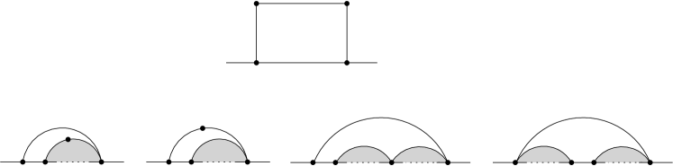
Figure 11: Possible faces incident to a boundary edge for quadrangulations. The first three may also be reflected to give the 8 topologically distinct possibilities. The holes (shaded) can have boundary of any even length.

To get existence of the measures $\mathbb{H}^{(p)}_{\alpha}$, we need to show that for any $\gamma=\alpha^{1/(p-2)}$ there exists a $\beta$ so that $R(\beta,\gamma)$ as defined in (3.9) equals 1. By monotonicity, and since $R(0,\gamma)=\gamma^{p-2}<1$ (the only term with no power $\beta$ corresponds to the event $A_{p-2}$ with probability $\alpha$), it suffices to show that some $\beta$ satisfies $1\leq R(\beta,\gamma)<\infty$. Note that just from steps of type $A_{0}$ and $A_{p-2}$ we get $R(\beta,\gamma)\geq\beta^{p-2}+\gamma^{p-2}$. Thus for $\beta$ close to $1$ we have $R(\beta,\gamma)>1$, provided it is finite. We prove this holds at least for $\alpha$ sufficiently close to $1$:

Proposition 3.11.

For any $p\geq 4$, and any $\alpha\in(\alpha_{0}(p),1)$ there is some $\beta$ so that $R(\beta,\alpha^{1/(p-2)})>1$, and so the measure $\mathbb{H}^{(p)}_{\alpha}$ exists for $\alpha>\alpha_{0}(p)$.

Proof.

To see that $Z_{m}(q)<\infty$ for small enough $q$ we need that the number of $p$-angulations grows at most exponentially. For triangulations or even $p$ this is known from exact enumerative formulae. For any $p$-angulation we can partition each face into triangles to get a triangulation of the $m$-gon. The number of those is at most exponential in the number of vertices. The number of $p$-angulations corresponding to a triangulation is at most $2$ to the number of edges, as each edge is either in the $p$-angulation or not. Thus we get a (crude) exponential bound also for odd $p$.

It is easy to see that there exists a $0<q_{c}<1$ such that $Z_{m}(q)<\infty$ for $q<q_{c}\neq 0$. We expect $Z_{m}(q_{c})<\infty$ as well, though that is not necessary for the rest of the argument. Now we need some general estimate giving exponential growth of $Z_{m}$. Fix any $q<q_{c}$. Note that $\psi_{m,n}\geq\psi_{m+p-2,n-p+2}$ by just counting maps where the face containing the root is incident to no other boundary vertices. Thus $Z_{m}(q)\geq q^{p-2}Z_{m+p-2}(q)$, and so $Z_{m}(q)\leq Cq^{-m}$ for some constant $C>0$, provided it is finite. Of course, this crude bound does not give the correct rate of increase for $Z$ as $m\to\infty$.

In each term of (3.9), the $m_{i}-k_{i}$ are bounded, but while keeping them fixed, the $k_{i}$’s could take any value (subject to parity constraints for even $p$). Fixing $m_{i}-k_{i}$ and summing over the possibilities for the $k_{i}$’s we see that $R(\beta,\gamma)<\infty$ provided that $\sum_{m}\beta^{m}Z_{m}(\beta\gamma)<\infty$. Now $Z_{m}(q)$ is an increasing function of $q$ as long as it is finite since all the coefficients of $Z_{m}$ are non-negative integers. Thus we have for $\beta=q_{c}/(4\gamma)$, any choice of $\gamma>1/2$ and the estimate on $Z_{m}$ found above,

$$\sum_{m}\beta^{m}Z_{m}(\beta\gamma)=\sum_{m}\beta^{m}Z_{m}\left(\frac{q_{c}}{4}\right)<\sum_{m}\left(\frac{q_{c}}{4\gamma}\right)^{m}Z_{m}\left(\frac{q_{c}}{2}\right)<\sum_{m}(2\gamma)^{-m}<\infty$$ (3.10)

Thus for a choice of $\gamma$ close to $1$ and $\beta=q_{c}/4\gamma$ we have $R(\beta,\gamma)<\infty$ and $R(\beta,\gamma)\geq\beta^{p-2}+\gamma^{p-2}>1$.

Having found a $\gamma$ so that $R(\beta,\gamma)=1$, we know the probability that the map contains any given finite neighbourhood of the root. The rest of the construction is similar to the triangulation case as described in Section 3.2 with no significant changes. ∎

Based on the behavior in the case of $p=3$, we expect the measures $\mathbb{H}_{\alpha}$ to exist for all $\alpha<1$. Moreover, we expect that $R(q_{c}/\gamma,\gamma)>1$ when $\gamma^{p-2}=\alpha>\alpha_{c}$ and that for smaller $\gamma$ the maximal finite value taken by $R$ is exactly $1$ where $\alpha_{c}$ will be a critical value of $\alpha$ at which a phase transition occurs analogous to the triangulation case. We see below that $\mathbb{H}^{(4)}_{\alpha}$ exists for $\alpha\leq\frac{3}{8}$, and a similar argument holds for other even $p$ (when there are explicit enumeration results).

3.6 Non-simple $p$-angulations

Finally, let us address the situation with $p$-angulations with non-simple faces. In the case of $p$-angulations for $p>3$, uniqueness breaks down thoroughly, and a construction similar to Section 3.4 applies. For even $p$ self-loops are impossible since a $p$-angulation is bi-partite. However, inspection of the construction of $\mathbb{H}_{\alpha,q,\nu}$ shows that it works not because of the self-loop, but because it is possible for a single face to completely surround other faces of the map.

Consider first the case $p=4$, and suppose we are given a measure $\mu$ supported on $\mathcal{H}_{4}$ satisfying translation invariance and the domain Markov property. Take a sample from $\mu$, and replace each edge by an independent geometric number of parallel edges. In each of the $2$-gons created, add another $2$-gon attached to one of the two vertices with equal probability, thereby creating a quadrangle. Fill the smaller $2$-gons with i.i.d. samples from an arbitrary distribution supported on quadrangulations of $2$-gons (see Figure 12). As with triangulations, this results in a measure which is domain Markov and translation invariant.

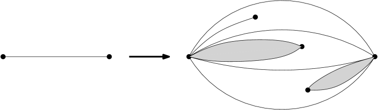
Figure 12: Non-uniqueness for quadrangulations: each edge is replaced with a geometric number of parallel edges. In each $2$-gon an internal $2$–gon is added at a uniformly chosen endpoint, and filled with an independent finite (possibly empty) quadrangulation.

Hence we see that faces which completely surround other faces of the map prevent us from getting only a one-parameter family of domain Markov measures. For triangulations and quadrangulations, the external boundary of such a face can only consist of $2$ edges (i.e. there are precisely two edges connecting the face to the infinite component of the complement). Removing such faces and identifying the two edges results in a domain Markov map with simple faces, which falls into our classification. Similarly to Proposition 3.8, it is possible to get a complete characterization of all domain Markov maps on quadrangulations in terms of $\alpha$, the density $\gamma$ of non-simple faces, and a measure $\nu$ on quadrangulations in a $2$-gon.

For $p\geq 5$, things get messier. Similar constructions work for any $p>3$, with inserted $2$-gons for even $p$, and any combination of $2$-gons and self-loops for $p$ odd. However, here this no longer gives all domain Markov $p$-angulations. A non-simple face can have external boundary of any size from $2$ up to $p-1$ (with parity constraint for even $p$). Thus it is not generally possible to get a $p$-angulation with simple faces from a general one. Removing the non-simple faces leaves a domain Markov map with simple faces of unequal sizes. It is possible to classify such maps, and these are naturally parametrized by a finite number of parameters, since we must also allow for the relative frequency of different face sizes. Much of such a classification is similar to the proofs of Theorems 1.2 and 3.1, and we do not pursue this here.

4 Approximation by finite maps

We prove Theorem 1.4, identifying the local limits of uniform measures on finite triangulations in this section. Here, we are concerned only with the measures $\mathbb{H}_{\alpha}$ on triangulations for critical and sub-critical $\alpha\leq 2/3$. Recall from the statement of the theorem, that we have sequences $(m_{l})_{l\in\mathbb{N}}$, $(n_{l})_{l\in\mathbb{N}}$ of integers such that $m_{l}/n_{l}\rightarrow a$ for some $a\in[0,\infty]$ and $m_{l},n_{l}\to\infty$. We show that $\mu_{m_{l},n_{l}}$ — the uniform measure on triangulations of an $m$-gon with $n$ internal vertices — converges weakly to $\mathbb{H}_{\alpha}$ where $\alpha=\frac{2}{2a+3}$. To simplify the notation, we drop the index $l$ from the sequences $m_{l}$ and $n_{l}$ and assume that $m$ is implicitly a function of $n$. Note that since $[0,\infty]$ is compact, it follows that $\{\mathbb{H}_{\alpha}\}_{\alpha\leq 2/3}$ are all the possible local limits of the $\mu_{m,n}$s.

Here is an outline of the proof: A direct computation shows that the $\mu_{m,n}$ measure of the event that the hull of the ball of radius $r$ is a particular finite triangulation $T$ converges to the $\mathbb{H}_{\alpha}$ measure of the same event (for any $T$), as given by Lemma 3.7. While a priori this only gives convergence in the vague topology, since the limit $\mathbb{H}_{\alpha}$ is a probability measure, it actually follows that $\mu_{m,n}$ is a tight family of measures and hence converges weakly. Thus we show the convergence of the hulls of balls. Note that the hulls of balls around the root always have a simple boundary.

We start with a simple estimate on relative enumerations on the number of triangulations of a polygon.

Lemma 4.1.

Suppose $m,n\to\infty$ so that $m/n\to a$ for some $a\in[0,\infty]$. Then for any fixed $j,k\in\mathbb{Z}$,

$$\lim_{n,m\to\infty}\frac{\phi_{n-k,m-j}}{\phi_{n,m}}=\left(\frac{(a+1)^{2}}{(2a+3)^{2}}\right)^{j}\left(\frac{2(a+1)^{2}}{(2a+3)^{3}}\right)^{k}$$

Proof.

By applying Stirling’s approximation to (2.1), we have for $m,n$ large

$$\phi_{n,m+2} =\frac{2^{n+1}(2m+1)!(2m+3n)!}{(m!)^{2}n!(2m+2n+2)!}$$

$$\sim c_{1}\frac{2^{n+1}(2m+1)!}{(m!)^{2}}\left(\frac{(2m+3n)^{2m+3n+1/2}}{(2m+2n+2)^{2m+2n+5/2}n^{n+1/2}}\right)$$

$$\sim c_{2}2^{n}4^{m}\sqrt{m}\left(\frac{27}{4}\right)^{n}\left(\frac{9}{4}\right)^{m}n^{-5/2}\left(1+\frac{2m}{3n}\right)^{2m+3n}\left(1+\frac{m}{n}\right)^{-2m-2n}$$

Taking the ratio, we have

$$\frac{\phi_{n-k,m+2-j}}{\phi_{n,m+2}}\sim\left(\frac{2}{27}\right)^{k}\left(\frac{1}{9}\right)^{j}\frac{(1+\frac{m}{n})^{2j+2k}}{(1+\frac{2m}{3n})^{2j+3k}}\quad\times\\ \left(\frac{1+\frac{2m-2j}{3n-3k}}{1+\frac{2m}{3n}}\right)^{2m+3n}\left(\frac{1+\frac{m-j}{n-k}}{1+\frac{m}{n}}\right)^{-2m-2n}.$$ (4.1)

An easy calculation shows that the product of the last two terms in the right hand side of (4.1) converges to $1$. Indeed, if $a$ is finite then the first tends to $e^{-2j+2ak}$ and the second to $e^{2j-2ak}$. If $a=\infty$ then after shifting a factor of $\left(\frac{n}{n-k}\right)^{2m}$ from the first to the second, the limits are $e^{-2j}$ and $e^{2j}$.

The result follows by taking the limit and using the fact that $m/n$ converges to $a$. ∎

Let $A_{Q},V(Q),F(Q),V(B)$ be as in Lemma 3.2, and note that $A_{Q}$ makes sense also when looking for $Q$ as a sub-map of a finite map.

Lemma 4.2.

Suppose $m,n\to\infty$ with $m/n\rightarrow a$ for some $a\in[0,\infty]$. Then

$$\lim_{m,n}\mu_{m,n}(A_{Q})=\left(\frac{2}{2a+3}\right)^{V(Q)-V(B)}\left(\frac{a+1}{2a+3}\right)^{2(F(Q)-V(Q)+V(B))}.$$

Remark 4.3.

If we make the change of variable $\alpha=2(2a+3)^{-1}$, then Lemma 4.2 gives us

$$\lim_{m,n}\mu_{m,n}(A_{Q})=\alpha^{V(Q)-V(B)}\left(\frac{(2-\alpha)^{2}}{16}\right)^{(F(Q)-V(Q)+V(B))}.$$

From Lemma 4.2 we can immediately conclude that the $\mu_{m,n}$-measure of $A_{Q}$ converges to the $\mathbb{H}_{\alpha}$ measure of the corresponding event.

Corollary 4.4.

Suppose $m,n\to\infty$ with $m/n\rightarrow a$ for some $a\in[0,\infty]$. Then we have

$$\lim_{m,n}\mu_{m,n}(A_{Q})=\mathbb{H}_{\alpha}(A_{Q})$$

where $\alpha=\frac{2}{2a+3}$.

Proof of Lemma 4.2.

It is clear that the number of simple triangulations of an $m+2$-gon with $n$ internal vertices where $A_{Q}$ occurs is $\phi_{n-k,m+2-j}$ where $j=2V(B)-|\partial Q|-2$ where $|\partial Q|$ is the number of vertices in the boundary of $Q$, and $k=V(Q)-V(B)$. Then from Lemma 4.1, we have

$$\lim_{m,n}\mu_{m,n}(A_{Q})=\lim_{n,m}\frac{\phi_{n-k,m+2-j}}{\phi_{n,m+2}}=\left(\frac{(1+a)^{2}}{(2a+3)^{2}}\right)^{j}\left(\frac{2(a+1)^{2}}{(2a+3)^{3}}\right)^{k}$$

From Euler’s formula, it is easy to see that $F(Q)=2V(B)-|\partial Q|-2$. This shows $j+k=F(Q)-V(Q)+V(B)$. Using all this, we have the Lemma. ∎

Proof of Theorem 1.4.

Corollary 4.4 gives convergence for cylinder events. Since $\mathbb{H}_{\alpha}$ is a probability measure, the result follows by Fatou’s lemma. ∎

4.1 Quadrangulations and beyond

Can we get similar finite approximations for $\mathbb{H}_{\alpha}^{(p)}$ for $p>3$? We think it is possible to prove such results based on enumeration of general $p$-angulations with a boundary, which is available for $p$ even. We believe that similar results should hold for any $p$, though do not see a way to prove them. Let us present here a recipe for quadrangulations. For higher even $p$ there are additional complications as the core is no longer a $p$-angulation and results on maps with mixed face sizes are needed.

Let us first consider quadrangulations with a simple boundary. Denote by $\mathcal{Q}_{2m,n}$ the space of quadrangulations with simple boundary size $2m$ and number of internal vertices $n$ (note that since the quadrangulation is bipartite, the boundary size is always even). Let $q_{2m,n}=\#\mathcal{Q}_{2m,n}$ be its cardinality. Enumerative results are available in this situation (see [14]). We alert the reader that our notation is slightly different from [14]: they use $\tilde{q}_{2m,n}$ for quadrangulations with a simple boundary and $n$ denotes the number of faces, not the number of internal vertices. Using Euler’s formula one can easily change from one variable to the other. Doing that, we get:

$$q_{2m,n}=3^{n-1}\frac{(3m)!}{m!(2m-1)!}\frac{(2n+3m-3)!}{n!(n+3m-1)!}$$ (4.2)

Now suppose $m/n\to a$ for some $a\in[0,\infty]$ where $m$ and $n$ are sequences such that $m\to\infty$ and $n\to\infty$. Let $\nu_{2m,n}$ be the uniform measure on all quadrangulations of boundary size $2m$ and $n$ internal vertices. A straightforward computation similar to Lemmas 4.1 and 4.2 gives us for any finite $Q$,

$$\lim_{m,n}\nu_{2m,n}(A_{Q})=\left(\frac{4(1+3a)^{3}}{27(2+3a)^{3}}\right)^{F(Q)}\cdot\left(\frac{9(2+3a)}{4(1+3a)^{2}}\right)^{V(Q)-V(B)}$$ (4.3)

where $V(Q)$ is the number of vertices in $Q$, $V(B)$ is the number of vertices of $Q$ on the boundary of $M$, and $F(Q)$ is the number of faces in $Q$ (by Euler’s characteristic, the “change” in the boundary length when removing $Q$ is $2(V(Q)-V(B)-F(Q))$).

The limit (4.3) in itself is not enough to give us distributional convergence of $\nu_{2m,n}$, as we are missing tightness. It is possible to get tightness for $\nu_{2m,n}$ using the same ideas presented for example in [7, 21] or the general approach found in [12]. The key is that it suffices to show the tightness of the root degree. The interested reader can work out the details and we shall not go into them here. Instead, throughout the remaining part of this section, we shall assume that the distributional limits of $\nu_{2m,n}$ exist. We remark here that when $a=0$ the limiting measures of the events described by (4.3) matches exactly with that of the half planar UIPQ measure (see [17]) and that for $a=\infty$ we get the dual of a critical Galton-Watson tree conditioned to survive. Thus in these two extreme cases, the distributional limit has already been established.

To handle all $a$, we define the operator $\operatorname{core}:\mathcal{H}_{4}\to\mathcal{H}^{\prime}_{4}$, which is the reverse of the process used to define the measures $\mathbb{H}_{\alpha,q,\nu}$ in Section 3.4, and acts on the dual by taking the $2$-connected core. Formally, any face which is not simple must have an external double edge connecting it to the rest of the map (and a $2$-gon inside it). The $\operatorname{core}$ operator removes every such face, and identifies the two edges connecting it to the outside. This operation is defined in the same way on quadrangulations of an $m$-gon. As discussed in Section 3.4, if $\mu$ is domain Markov on $\mathcal{H}_{4}$ then $\mu\circ\operatorname{core}^{-1}$ is domain Markov on $\mathcal{H}^{\prime}_{4}$.

Let $\mu=\lim\nu_{2m,n}$ as $m,n\to\infty$ with $m/n\to a\in[0,\infty]$. We first observe that $\mu$ is domain Markov and translation invariant. This follows from (4.3) and the converse part of Lemma 3.10.

Next, observe that the events $A_{i}$ for $i=0,1,2$ are not affected by $\operatorname{core}$. This is because in each of them, the face containing the root is a simple face, and so is not contained in any non-simple face. At this point from (4.3), we obtain $\beta^{2}=(4(1+3a)^{3})/(27(2+3a)^{3})$ and $\gamma/\beta=(9(2+3a))(4(1+3a)^{2})$. Thus,

$$\mu(A_{2}) =\frac{3}{4(1+3a)(2+3a)} \mu(A_{0}) =\frac{4}{27}\left(\frac{1+3a}{2+3a}\right)^{3}.$$

From the first we see that as $a$ goes from $0$ to $\infty$ we get $\alpha\in[0,\frac{3}{8}]$. Solving for $a$ in terms of $\alpha=\mu(A_{2})$ and plugging in we find $\beta=\sqrt{\mu(A_{0})}=\frac{2}{27}(\sqrt{3+\alpha}-\sqrt{\alpha})^{3}$, which decreases from $\sqrt{4/27}$ to $\sqrt{1/54}$ as $\alpha$ increases from $0$ to $3/8$.

This gives the measures $\mathbb{H}^{(4)}_{\alpha}$ as the the core of the limit of uniform measures on non-simple quadrangulations. Since the core operation is continuous in the local topology, this is also the limit of the core of uniform quadrangulations. This does not give $\mathbb{H}^{(4)}_{\alpha}$ as a limit of uniform measures on non-simple quadrangulations, since the number of internal vertices in the core of a uniform map from $\mathcal{Q}_{2m,n}$ is not fixed. Thus the above only proves the limit when $n$ is taken to be random with a certain distribution (though concentrated and tending to infinity in proportion to $m$.) It should be possible to deduce that uniform simple quadrangulations converge to $\mathbb{H}^{(4)}_{\alpha}$ by using a local limit theorem for the distribution of the size of the core (see [8, 9]). We leave these details to the readers.

The above indicates that a phase transition for the family $\mathbb{H}_{\alpha}^{(4)}$ occurs at $\alpha=3/8$, similar to the case $p=3$. We can similarly compute the asymptotics of $p_{k}$ as in Section 3.3 and see that $p_{k}\sim ck^{-5/2}$ for $\alpha=3/8$ and $p_{k}\sim ck^{-3/2}$ for $\alpha<3/8$. This indicates different geometry of the maps. All these hints encourage us to conjecture that a similar picture of phase transition do exist for the measures $\mathbb{H}_{\alpha}^{(p)}$ for all $p>3$.

Omer Angel, UBC, <angel@math.ubc.ca>
Gourab Ray, UBC, <gourab1987@gmail.com>

References

- [1] J. Ambjorn. Quantization of geometry. 1994 Les Houches Summer School “Fluctuating Geometries in Statistical Mechanics and Field Theory”, 1994.
- [2] J. Ambjørn, B. Durhuus, and T. Jonsson. Quantum Gravity, a Statitstical Field Theory Approach. Cambridge Monographs on Mathematical Physics, 1997.
- [3] O. Angel. Growth and percolation on the uniform infinite planar triangulation. Geom. Funct. Anal., 13(5):935–974, 2003.
- [4] O. Angel. Scaling of percolation on infinite planar maps, i. http://arxiv.org/abs/math/0501006, 2005.
- [5] O. Angel and N. Curien. Percolations on random maps I: half-plane models. http://arxiv.org/abs/1301.5311, 2013.
- [6] O. Angel and G. Ray. Geometry of domain Markov half planar triangulations. in preparation, 2013.
- [7] O. Angel and O. Schramm. Uniform infinite planar triangulations. Comm. Math. Phys., 241(2-3):191–213, 2003.
- [8] C. Banderier, P. Flajolet, G. Schaeffer, and M. Soria. Planar maps and Airy phenomena. In Automata, languages and programming (Geneva, 2000), volume 1853 of Lecture Notes in Comput. Sci., pages 388–402. Springer, Berlin, 2000.
- [9] C. Banderier, P. Flajolet, G. Schaeffer, and M. Soria. Random maps, coalescing saddles, singularity analysis, and Airy phenomena. Random Structures Algorithms, 19(3-4):194–246, 2001. Analysis of algorithms (Krynica Morska, 2000).
- [10] I. Benjamini. Euclidean vs graph metric. www.wisdom.weizmann.ac.il/ itai/erd100.pdf.
- [11] I. Benjamini and N. Curien. Simple random walk on the uniform infinite planar quadrangulation: Subdiffusivity via pioneer points. http://arxiv.org/abs/1202.5454, 2012.
- [12] I. Benjamini, R. Lyons, and O. Schramm. Unimodular random trees. http://arxiv.org/abs/1207.1752, 2012.
- [13] I. Benjamini and O. Schramm. Recurrence of distributional limits of finite planar graphs. Electron. J. Probab., 6:no. 23, 1–13, 2001.
- [14] J. Bouttier and E. Guitter. Distance statistics in quadrangulations with a boundary, or with a self-avoiding loop. J. Phys. A, 42(46):465208, 44, 2009.
- [15] E. Brezin, C. Itzykson, G. Parisi, and J. Zuber. Planar diagrams. Comm. Math. Phys., 59:35–51, 1978.
- [16] N. Curien, L. Ménard, and G. Miermont. A view from infinity of the uniform infinite planar quadrangulation. http://arXiv.org/abs/1201.1052.
- [17] N. Curien and G. Miermont. Uniform infinite planar quadrangulations with a boundary. http://arXiv.org/abs/1202.5452, 2012.
- [18] I. P. Goulden and D. M. Jackson. Combinatorial enumeration. A Wiley-Interscience Publication. John Wiley & Sons Inc., New York, 1983. With a foreword by Gian-Carlo Rota, Wiley-Interscience Series in Discrete Mathematics.
- [19] O. Gurel-Gurevich and A. Nachmias. Recurrence of planar graph limits. Annals of Mathematics, 177 no. 2:761–781, 2013.
- [20] V. G. Knizhnik, A. M. Polyakov, and A. B. Zamolodchikov. Fractal structure of 2D-quantum gravity. Modern Phys. Lett. A, 3(8):819–826, 1988. http://dx.doi.org/10.1142/S0217732388000982.
- [21] M. Krikun. Local structure of random quadrangulations. http://arxiv.org/abs/math/0512304, 2005.
- [22] S. Lando and A. Zvonkin. Graphs on surfaces and their applications. Encyclopedia of Mathematical Sciences, Springer, Berlin, 141, 2004.
- [23] H. Ren, Y. Liu, and Z. Li. Enumeration of 2-connected loopless 4-regular maps on the plane. European J. Combin., 23(1):93–111, 2002.
- [24] G. Schaffer. Conjugaison d’arbres et cartes combinatoires aléatoires. PhD thesis, 1998.
- [25] O. Schramm. Scaling limits of loop-erased random walks and uniform spanning trees. Israel J. Math., 118:221–288, 2000.
- [26] G. ’t Hooft. A Planar Diagram Theory for Strong Interactions. Nucl. Phys., B72:461, 1974.
- [27] W. T. Tutte. A census of planar triangulations. Canad. J. Math., 14:21–38, 1962.
- [28] Y. Watabiki. Construction of non-critical string field theory by transfer matrix formalism in dynamical triangulation. Nuclear Phys. B, 441(1-2):119–163, 1995.