Phase Transition Analysis of Sparse Support Detection from Noisy Measurements

Abstract

This paper investigates the problem of sparse support detection (SSD) via a detection-oriented algorithm named Bayesian hypothesis test via belief propagation (BHT-BP) [7],[8]. Our main focus is to compare BHT-BP to an estimation-based algorithm, called CS-BP [3], and show its superiority in the SSD problem. For this investigation, we perform a phase transition (PT) analysis over the plain of the noise level and signal magnitude on the signal support. This PT analysis sharply specifies the required signal magnitude for the detection under a certain noise level. In addition, we provide an experimental validation to assure the PT analysis. Our analytical and experimental results show the fact that BHT-BP detects the signal support against additive noise more robustly than CS-BP does.

I Introduction

Noisy sparse recovery is referred to the problem of recovering a sparse signal $\mathbf{x}_{0}\in\mathbb{R}^{N}$ from noisy linear projection $\mathbf{y}\in\mathbb{R}^{M}$ generated by an underdetermined system $(M<N)$. In such a problem, sparse support detection (SSD) is important because once the support is known, the uncertainty to the recovery is confined to the additive noise, which can be optimally solved in terms of mean squared errors using the simple least square approach [1]. Nevertheless, most recovery algorithms to date for the problem have been developed under the auspices of signal estimation rather than support detection. They include algorithms developed under the criteria of the $l_{1}$-norm minimization and the MAP-estimation such as least absolute shrinkage and selection operator (LASSO) [2] and Baysian compressive sensing via belief propagation (CS-BP) [3], respectively.

Thus, we make note of the fact that these estimation-based algorithms may not be good choices when it comes to the SSD problem under noisy setup. Indeed, recently several studies have indicated that the existing estimation-based algorithms lead to a potentially large gap with respect to the theoretical limit for the noisy support recovery [4]-[6]. Wainwright and Akcakaya et al. have shown that LASSO, a sparse signal estimator, has a significant performance gap from the Fano’s detector which is information-theoretically optimal, in the linear sparsity regime [4],[5]. Furthermore, Fletcher et al. noted the suboptimality of LASSO and OMP compared to the maximum likelihood detector and they remarked that the gap grows as SNR increases [6].

In this paper, we consider a recently proposed detection-oriented algorithm named Bayesian hypothesis test via belief propagation (BHT-BP) [7],[8]. This algorithm detects the signal support through a sequence of binary hypothesis tests, where each hypothesis test is designed from the MAP-detection criterion using Bayesian philosophy. In our previous studies [7],[8], we have shown in extensive simulation that BHT-BP works better than the estimation-based algorithms, such as CS-BP and LASSO, for the SSD problem, particularly when situations are noisy. In addition, we noted that BHT-BP is noteworthy as a low-computational algorithm having $O(N\log N)$ order of complexity, enabled by belief propagation (BP) working on sparse measurement matrices. In those studies, however, the superiority of BHT-BP to the estimation-based algorithms was verified only in simulation.

The main focus of this paper is to introduce a phase transition (PT) analysis which can be used to describe how the support detection of the BHT-BP algorithm behaves as the additive noise level is varied. Namely, it provides an exact border line between success and failure of the algorithm on the plane of the noise level and the signal magnitude. The term “phase transition” was first used by Donoho and Tanner [9],[10] in the sparse recovery literature, where the relation between the undersampling ratio and the signal sparsity was the focus which is different from the work studied here.

The importance of the signal magnitude, the smallest magnitude on the support to be more precise, in noisy sparse recovery problems has been emphasized in [4],[6] where they have shown that the required number of compressive measurements for support detection is inversely proportional to the power of the smallest magnitude on the support. Their study, however, did not answer the following question: for successful support detections, how large should the signal magnitude be at a fixed noise level? With the PT analysis in this paper, such a statement can be made sharp. In addition, in order to verify the superiority of the detection-oriented algorithm BHT-BP to the estimation-based one CS-BP, we compare the PT region of BHT-BP to that of CS-BP. The comparisons are made both in analysis and simulations which confirm that the PT region of BHT-BP is larger than that of CS-BP.

Figure 1: Channel model for sparse support detection

II Problem Formulation

II-A Signal Model

We consider a sparse signal $\mathbf{x}_{0}\in\mathbb{R}^{N}$ which is a realization of a random vector $\mathbf{X}$. Here we assume that the elements of $\mathbf{X}$ are i.i.d. and that the supportive state of each $X_{i}$ is determined by a Bernoulli random variable $S_{i}$ with a mixing rate $q:=\Pr\{S_{i}=1\}$, i.e.,

$${S_{i}}=\left\{\begin{array}[]{l}1,\,\,\,\,\,{\text{if}}\,\,\ X_{i}\neq 0\\ 0,\,\,\,\,\,{\text{else}}\end{array}\right.\forall\,\,i\in\{1,...,N\}.$$ (3)

Hence, the state vector $\mathbf{S}\in\{0,1\}^{N}$ fully contains the support information on the signal $\mathbf{X}$. For nonzero values, we consider equiprobable signed values i.e., $X_{i|S_{i}=1}\sim\frac{1}{2}{\delta_{+{x}}}+\frac{1}{2}{\delta_{-{x}}}$ where $\delta_{\tau}$ denotes the delta function peaked at $\tau$.

Then, the support detector observes a noisy measurement vector, i.e.,

$$\mathbf{y}=\mathbf{\Phi}\mathbf{x}_{0}+\mathbf{w}\in\mathbb{R}^{M},$$ (4)

where we use sparse measurement matrices $\mathbf{\Phi}\in\{0,1\}^{M\times N}$ whose matrix sparsity is regulated by its fixed column weight, i.e., $\left|\{j:\phi_{ji}\neq 0\}\right|=L$, and a zero-mean Gaussian vector $\mathbf{w}\in\mathbb{R}^{M}$ drawn from $\mathcal{N}(0,\sigma_{W}^{2}\mathbf{I})$ to represent additive white noise.

In the SSD problem, we assume a spike-and-slab prior such that for each signal element $X_{i}$, it is given by

$$\begin{array}[]{l}f_{X_{i}}(x):=qf_{X_{i}}(x|S_{i}=1)+(1-q)f_{X_{i}}(x|S_{i}=0)\\ \,\,\,\,\,\,\,\,\,\,\,\,\,\,\,\,\,\,\,=q\mathcal{N}(x;0,\sigma_{X}^{2})+(1-q)\delta_{0},\end{array}$$ (7)

where we use $f(\cdot)$ to denote a probability density function (PDF). The variance $\sigma_{X}^{2}$ is calibrated according the magnitude of the target signal $\mathbf{x}_{0}$. Namely, if the signal has large values on its support, the variance $\sigma_{X}^{2}$ should be sufficiently large for the support detection.

II-B Channel Model

Signal support detection can be performed in an elementwise manner on the basis of decoupling principle [11],[12]. According to this principle, the vector measurement channel can be decoupled to a sequence of scalar Gaussian channels in the large system limit ($N\rightarrow\infty$). In this case, the input of each elementwise support detection is a scalar estimate of $X_{i}$ denoted by $Z_{i}$, as shown in Fig.1.

The decoupling for the elementwise detection can be achieved using an iterative BP algorithm. Indeed, Guo and Wang have shown that the BP algorithm finds the marginal posteriors of the signal exactly if the matrix $\mathbf{\Phi}$ is assumed to be a sparse matrix with the no-short-cycle property [13]. Such a setting is called large-sparse-system (LSS) setup. Fig.1 shows the overall channel model considered in this paper in which we assume that the signal length $N$ is sufficiently large to justify the LSS setup.

II-C Problem Statement

In this study, we aim to analytically compare the noisy behavior of the two types of algorithms: BHT-BP and CS-BP. The CS-BP algorithm is an estimation-based algorithm which obtains the signal estimate directly from the posterior density of $\mathbf{Z}\in\mathbb{R}^{N}$ using the MAP or the MMSE estimator [3]. Therefore, in CS-BP, the support information is provided as a by-product of the signal estimate. Namely, if a scalar estimate given by $Z_{i}$ is nonzero, then the algorithm simply decides the element belongs to the signal support. Accordingly, the detection function for a supportive state $S_{i}$ in CS-BP is described by

$$h_{\text{CS-BP},i}:=\log\frac{{{f_{{X_{i}}}}(x={{\widehat{x}}_{\text{MAP},i}}|{Z_{i}},\mathbf{\Phi})}}{{{f_{{X_{i}}}}(x=0|{Z_{i}},\mathbf{\Phi})}}\mathop{\mathop{\gtrless}\limits_{{\mathcal{H}_{0}}}}\limits^{{\mathcal{H}_{1}}}0,$$ (8)

where $\mathcal{H}_{0}:=\{S_{i}=0\}$ and $\mathcal{H}_{1}:=\{S_{i}=1\}$ denote two possible hypotheses, and we assume CS-BP uses the MAP-estimator such that an estimate of $X_{i}$ is given as ${\widehat{x}_{\text{MAP},i}}:=\arg\mathop{\max}\limits_{x\neq 0}{f_{{X_{i}}}}(x|Z_{j},{\bf{\Phi}})$. The detection in (8) can be achieved with the marginal posterior ${f_{{X_{i}}}}(x|\mathbf{Y},{\bf{\Phi}})$ since

$${f_{{X_{i}}}}(x|{Z_{j}},{\bf{\Phi}})=\int\limits_{\bf{Y}}{\underbrace{{f_{{X_{i}}}}(x|{Z_{j}},{\bf{Y}},{\bf{\Phi}})}_{={f_{{X_{i}}}}(x|{\bf{Y}},{\bf{\Phi}})}{f_{\bf{Y}}}({\bf{y}}|{Z_{i}},{\bf{\Phi}})d{\bf{y}}},$$ (9)

and $f_{\bf{Y}}({\bf{y}}|{Z_{i}},{\bf{\Phi}})\geq 0$ for all $\mathbf{y}$ where $f_{X_{i}}(x|\mathbf{Y},Z_{i},{\bf{\Phi}})=f_{X_{i}}(x|\mathbf{Y},{\bf{\Phi}})$ is true because $Z_{i}$ is a function of $\mathbf{Y}$. Therefore, (8) can be rewritten as

$$h_{\text{CS-BP},i}=\log\frac{{{f_{{X_{i}}}}(x={{\widehat{x}}_{\text{MAP},i}}|{\bf{Y}},\mathbf{\Phi})}}{{{f_{{X_{i}}}}(x=0|{\bf{Y}},\mathbf{\Phi})}}\mathop{\mathop{\gtrless}\limits_{{\mathcal{H}_{0}}}}\limits^{{\mathcal{H}_{1}}}0.$$ (10)

In contrast, for a detection-oriented algorithm BHT-BP, finding the sparse support set is an end in itself. Therefore, the detection function of BHT-BP is designed from the MAP-detection of the supportive state $S_{i}$, given by

$$h_{\text{MAP},i}:=\log\frac{{\Pr\{{S_{i}}=1|Z_{i},{\bf{\Phi}}\}}}{{\Pr\{{S_{i}}=0|Z_{i},{\bf{\Phi}}\}}}\mathop{\mathop{\gtrless}\limits_{{\mathcal{H}_{0}}}}\limits^{{\mathcal{H}_{1}}}0.$$ (11)

In (11), the posterior probability of a supportive state $S_{i}$ can be decomposed as

$$\Pr\{{S_{i}}|{Z_{i}},{\bf{\Phi}}\}$$

$$=\int\limits_{{X_{i}},{\bf{Y}}}\underbrace{\Pr\{{S_{i}}|{X_{i}},{\bf{Y}},{Z_{i}},{\bf{\Phi}}\}}_{=\Pr\{{S_{i}}|{X_{i}},{\bf{\Phi}}\}}\underbrace{{f_{{X_{i}}}}(x|{Z_{j}},{\bf{Y}},{\bf{\Phi}})}_{={f_{{X_{i}}}}(x|{\bf{Y}},{\bf{\Phi}})}\times$$

$$\,\,\,\,\,\,\,\,\,\,\,\,\,\,\,\,\,\times{f_{\bf{Y}}}({\bf{y}}|{Z_{i}},{\bf{\Phi}})dxd{\bf{y}}$$

$$=\int\limits_{\bf{Y}}{\left[{\int\limits_{{X_{i}}}{\frac{{{f_{{X_{i}}}}(x|{S_{i}})\Pr\{{S_{i}}\}{f_{{X_{i}}}}(x|{\bf{Y}},{\bf{\Phi}})}}{{{f_{{X_{i}}}}(x)}}dx}}\right]{f_{\bf{Y}}}({\bf{y}}|{Z_{i}},{\bf{\Phi}})}d{\bf{y}},$$ (12)

where $\Pr\{{S_{i}}|{X_{i}},{\bf{Y}},{Z_{i}},{\bf{\Phi}}\}=\Pr\{{S_{i}}|{X_{i}},{\bf{\Phi}}\}$ holds true because $Z_{i}$ and $\mathbf{Y}$ are conditionally independent of $S_{i}$ given $X_{i}$. In addition, we know from (9) that $f_{X_{i}}(x|\mathbf{Y},Z_{i},{\bf{\Phi}})=f_{X_{i}}(x|\mathbf{Y},{\bf{\Phi}})$. Therefore, the MAP-detection can be achieved by considering only the integral within brackets since $f_{\bf{Y}}({\bf{y}}|{Z_{i}},{\bf{\Phi}})\geq 0$ for all $\mathbf{y}$. Using these facts, the detection function of BHT-BP is defined as

$$h_{\text{BHT-BP},i}:=\log\frac{q}{1-q}+\log{\frac{{\int{\frac{{f_{X_{i}}(x|S=1)}}{{f_{X_{i}}(x)}}f_{X_{i}}(x|{\bf{Y}},{\bf{\Phi}})}dx}}{{\int{\frac{{f_{X_{i}}(x|S=0)}}{{f_{X_{i}}(x)}}f_{X_{i}}(x|{\bf{Y}},{\bf{\Phi}})}dx}}}\mathop{\mathop{\gtrless}\limits_{{\mathcal{H}_{0}}}}\limits^{{\mathcal{H}_{1}}}0.$$ (13)

These detection functions in (10) and (13) will be used later on for development of the PT analysis in Section III-B.

As the first step of this analysis, we provide an analytical expression of the marginal posterior ${f_{{X_{i}}}}(x|\mathbf{Y},{\bf{\Phi}})$ obtained via BP, under the LSS setup. This posterior expression is used to represent the detection function of CS-BP (10) and BHT-BP (13) as a function of $\sigma_{W}$ and $x_{0,i}$. Then, using this result, we analyze the failure event for each detection function and compare the condition for these two events over the plane of the noise level $\sigma_{W}$ and signal magnitude $x_{0,i}$. Our analytical and experimental results show that BHT-BP detects the signal support more robustly than CS-BP, for the given noise level $\sigma_{W}$ and signal magnitude $|x_{0,i}|$.

III Main Result

III-A Derivation of Marginal Signal Posterior

Let ${V^{(l)}_{{X_{i}}\to{Y_{j}}}}$ and ${U^{(l)}_{{Y_{j}}\to{X_{i}}}}$ represent the BP-messages passed from $X_{i}$ to $Y_{j}$ and from $Y_{j}$ to $X_{i}$, respectively, for all pairs of $(i,j):\phi_{ji}\neq 0$ at the $l$-th iteration. Our derivation starts from the message ${U^{(l)}_{{Y_{j}}\to{X_{i}}}}$, expressed as

$${U^{(l)}_{{Y_{j}}\to{X_{i}}}}=Y_{j}-\sum\limits_{\scriptstyle k:{\phi_{jk}}\neq 0,k\neq i}{{\bf{E}}\{{X_{k}}|{V^{(l-1)}_{{X_{k}}\to{Y_{j}}}},{\bf{\Phi}}\}}+N_{j}.$$ (14)

By the central limit theorem (CLT), as a sum of i.i.d. random variables, the message ${U_{{Y_{j}}\to{X_{i}}}}$ is asymptotically Gaussian under the LSS setup [13]. Then, we have

$${U^{(l)}_{{Y_{j}}\to{X_{i}}}}\mathop{\sim}\limits^{{\text{by CLT}}}\mathcal{N}\left(y_{j}-\sum\limits_{k}{{\bf{E}}\{{X_{k}}|{V^{(l-1)}_{{X_{k}}\to{Y_{j}}}},{\bf{\Phi}}\}},\sigma_{W}^{2}+\sigma_{\text{CEI}}^{2}\right),$$ (15)

where $\sigma_{\text{CEI}}^{2}$ denotes the variance of the cross-element-interference (CEI). In addition, we use the fact that the mean of the Gaussian PDF in (15) converges to the true value, i.e., $y_{j}-\sum\limits_{k}{{\bf{E}}\{{X_{k}}|{V^{(l-1)}_{{X_{k}}\to{Y_{j}}}},{\bf{\Phi}}\}}\rightarrow x_{0,i}$, and the interference term will be eliminated, i.e., $\sigma_{\text{CEI}}^{2}\rightarrow 0$, as the iteration becomes deeper $l\rightarrow\infty$ under the large system limit ($N\rightarrow\infty$) [13]. For the convergence of BP, we assume that the mixing rate $q$ is very small ($0<q\ll 1$) such that the signal is sparse enough. Accordingly, the PDF of messages from the measurement side toward $X_{i}$ converges to a Gaussian PDF with the mean $x_{0,i}$ and the variance $\sigma_{W}^{2}$, i.e.,

$$f_{{U_{{Y_{j}}\to{X_{i}}}}}(u|X_{i},\mathbf{Y},{\bf{\Phi}})\rightarrow\mathcal{N}(u;x_{0,i},\sigma_{W}^{2}).$$ (16)

As we discussed in Section II-B, the no-short-cycle property of the matrix $\mathbf{\Phi}$ ensures that elements of $\{{U_{{Y_{j}}\to{X_{i}}}}\}_{(i,j):\phi_{ji}\neq 0}$ are i.i.d. Then, using this property and the Bayesian rule, the marginal posterior of each $X_{i}$ is obtained as

$$f_{X_{i}}(x|\mathbf{Y},{\bf{\Phi}}) \mathop{\equiv}\limits^{{\text{by BP}}}{f_{{X_{i}}}}(x|{\bf{Y}},{\bf{\Phi}},{\bf{U}})$$ (17)

$$=\eta\left[f_{X_{i}}(x)\times\prod\limits_{j:\phi_{ji}\neq 0}f_{{U_{{Y_{j}}\rightarrow{X_{i}}}}}(u|X_{i},\mathbf{Y},{\bf{\Phi}})\right],$$

where $\eta[\cdot]$ is the normalization function ensuring $\int{f_{X_{i}}(x|\mathbf{Y},\mathbf{\Phi})dx=1}$. In addition, note that $|\{j:\phi_{ji}\neq 0\}|=L$ from our signal model; hence, the product in (17) is made up of $L$ densities for ${U_{{Y_{j}}\rightarrow{X_{i}}}}\,\,\forall j:\phi_{ji}\neq 0$. By applying the prior knowledge given in (7) and the result of (16) to (17), we have

$$f_{X_{i}}(x|\mathbf{Y},{\bf{\Phi}})$$

$$=\eta\left[qc_{2}\mathcal{N}(x;\frac{Lx_{0,i}\sigma_{X}^{2}}{L\sigma_{X}^{2}+\sigma_{W}^{2}},\frac{\sigma_{X}^{2}\sigma_{W}^{2}}{L\sigma_{X}^{2}+\sigma_{W}^{2}})+(1-q)c_{1}\delta_{0}\right],$$ (18)

where we use the fact that the product of Gaussian PDFs results in a scaled Gaussian PDF, i.e.,

$$\begin{array}[]{l}\mathcal{N}(x;{\mu_{1}},\sigma_{1}^{2})\times\mathcal{N}(x;{\mu_{2}},\sigma_{2}^{2})\propto\mathcal{N}(x;b,B),\end{array}$$

with $B=\frac{{\sigma_{1}^{2}\sigma_{2}^{2}}}{{\sigma_{1}^{2}+\sigma_{2}^{2}}},b=\frac{{{\mu_{1}}\sigma_{2}^{2}+{\mu_{2}}\sigma_{1}^{2}}}{{\sigma_{1}^{2}+\sigma_{2}^{2}}}$. Hence, the constants $c_{1},c_{2}$ in (III-A) are defined by

$$\begin{array}[]{l}c_{1}:=\exp\left[-\frac{Lx_{0,i}^{2}}{2\sigma_{W}^{2}}\right]/\sqrt{2\pi\sigma_{W}^{2}/L},\end{array}$$

and

$$\begin{array}[]{l}{c_{2}}:={{\exp\left[{\frac{{x_{0,i}^{2}}}{{2(\sigma_{X}^{2}+\sigma_{W}^{2}/L)}}}\right]}}/{{\sqrt{2\pi(\sigma_{X}^{2}+\sigma_{W}^{2}/L)}}}.\end{array}$$

The expression in (III-A) reveals that the marginal posterior consists of a slab-PDF $\mathcal{N}(x;\frac{Lx_{0,i}\sigma_{X}^{2}}{L\sigma_{X}^{2}+\sigma_{W}^{2}},\frac{\sigma_{X}^{2}\sigma_{N}^{2}}{L\sigma_{X}^{2}+\sigma_{W}^{2}})$ and a zero-spike $\delta_{0}$. For convenience, we define the mixing rate $\rho_{i}$, the mean $\mu_{i}$, and the variance $\theta_{i}^{2}$ of the marginal posterior as $\rho_{i}:=\frac{qc_{2}}{qc_{2}+(1-q)c_{1}}$, $\mu_{i}:=\frac{Lx_{0,i}\sigma_{X}^{2}}{L\sigma_{X}^{2}+\sigma_{W}^{2}}$, and $\theta_{i}^{2}:=\frac{\sigma_{X}^{2}\sigma_{N}^{2}}{L\sigma_{X}^{2}+\sigma_{W}^{2}}$, respectively. Then, using these parameters $\rho_{i},\mu_{i},\theta_{i}^{2}$, we can rewrite the marginal posterior in (III-A) as a spike-and-slab PDF, i.e.,

$$f_{X_{i}}(x|\mathbf{Y},{\bf{\Phi}})=\rho_{i}\mathcal{N}(x;\mu_{i},\theta_{i}^{2})+(1-\rho_{i})\delta_{0}.$$ (20)

Figure 2: Marginal posterior corresponding to noise level $\sigma_{W}$ when $q=0.05$, $\sigma_{X}=5$, $x_{0,i}=2.5$, and $L=4$ given $S_{i}=1$. The figure shows that the probability mass in the posterior spreads over the $x$-axis and approaches the prior PDF, as $\sigma_{W}$ increases.

III-B Phase Transition Analysis of Sparse Support Detection

We start the phase transition (PT) analysis from studying the behavior of the marginal posterior $f_{X_{i}}(x|\mathbf{Y},{\bf{\Phi}})$ corresponding to the noise level $\sigma_{W}$. We first examine the two extreme cases: $\sigma_{W}\rightarrow 0$ and $\sigma_{W}\rightarrow\infty$. In the noiseless setup, i.e., $\sigma_{W}\rightarrow 0$, the parameters of $f_{X_{i}}(x|\mathbf{Y},{\bf{\Phi}})$ converges to $\mathop{\lim}\limits_{{\sigma_{W}}\to 0}{\rho_{i}}=1,\mathop{\lim}\limits_{{\sigma_{W}}\to 0}{\mu_{i}}=x_{0,i},\mathop{\lim}\limits_{{\sigma_{W}}\to 0}{\theta_{i}}=0$. Therefore, the marginal posterior converges to a delta function peaked at $x_{0,i}$, i.e.,

$$\mathop{\lim}\limits_{{\sigma_{W}}\to 0}f_{X_{i}}(x|\mathbf{Y},{\bf{\Phi}})=\delta_{x_{0,i}}.$$ (21)

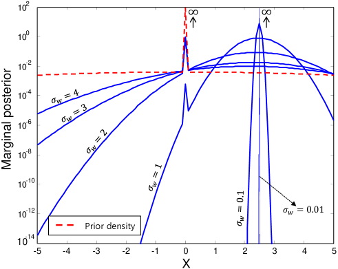
As $\sigma_{W}$ increases, the probability mass in the posterior spreads over the $x$-axis, as shown in Fig.2. In the extreme case, i.e., $\sigma_{W}\rightarrow\infty$, then the parameters converges to $\mathop{\lim}\limits_{{\sigma_{N}}\to\infty}{\rho_{i}}=q,\mathop{\lim}\limits_{{\sigma_{W}}\to\infty}{\mu_{i}}=0,\mathop{\lim}\limits_{{\sigma_{W}}\to\infty}{\theta_{i}}=\sigma_{X}$; hence, the marginal posterior converges to the prior PDF, i.e.,

$$\mathop{\lim}\limits_{{\sigma_{W}}\to\infty}f_{X_{i}}(x|\mathbf{Y},{\bf{\Phi}})=f_{X_{i}}(x).$$ (22)

Note that the results of (21) and (22) are independent of the other parameters ${\sigma_{{X}}},x_{0,i},q$. These facts indicate that, when the measurements $\mathbf{Y}$ are clean, the detection of the supportive state of $x_{0,i}$ can be achieved by either approach given in (13) or (10) without uncertainty, whereas in the extremely noisy case, the measurements $\mathbf{Y}$ are not at all useful for recovery of $x_{0,i}$, and the both approaches do not work for the support detection.

We now consider the failure event of the support detection. Let $\mathcal{F}_{i}$ denote the failure event of an index $i\in\{1,...,N\}$, i.e.,

$$\mathcal{F}_{i}:=\{\text{Decide}\,\mathcal{H}_{1},S_{i}=0\}\cup\{\text{Decide}\,\mathcal{H}_{0},S_{i}=1\},$$ (23)

which is the union of two possible failure cases in elementwise support detection. Let us consider the first case $\{\text{Decide}\,\mathcal{H}_{1},S_{i}=0\}$ in (23). For any zero element, i.e., $S_{i}=0$, it can be shown that the additive noise does not affect the success of the elementwise support detection. Namely, the state detection of $S_{i}=0$ is always right regardless of the noise level. $i)$ When the situation is noiseless, we know from (21) that the marginal posterior becomes the delta function peaked at the true value $x_{i,0}=0$. Therefore, it is obvious that

$$\arg\mathop{\max}\limits_{x}\mathop{\lim}\limits_{{\sigma_{N}}\to 0}{f_{{X_{i}}}}(x|{\bf{Y}},{\bf{\Phi}},{S_{i}}=0) =\arg\mathop{\max}\limits_{x}{\delta_{0}}$$

$$=0,$$ (24)

where the second line holds owing to the nature of the delta function $\delta_{0}$. $ii)$ The challenging case is when the noise level $\sigma_{W}$ is large. But, from (22), we have already seen that the marginal posterior converges to the prior density as $\sigma_{W}$ increases. Hence, clearly we have

$$\arg\mathop{\max}\limits_{x}\mathop{\lim}\limits_{{\sigma_{N}}\to\infty}{f_{{X_{i}}}}(x|{\bf{Y}},{\bf{\Phi}},{S_{i}}=0) =\arg\mathop{\max}\limits_{x}{f_{{X_{i}}}}(x)$$

$$=0,$$ (25)

where the second line holds by definition of the prior density given in (7). From $i)$ and $ii)$, the peak of $f_{X_{i}}(x|\mathbf{Y},{\bf{\Phi}},{S_{i}}=0)$ remains at $x=0$ regardless of the noise level, meaning that the state of any zero element having $S_{i}=0$, is detected perfectly with no failure, i.e., $\{\text{Decide}\,\mathcal{H}_{1},S_{i}=0\}=\emptyset$. Therefore, the failure event $\mathcal{F}_{i}$ is confined to the case $S_{i}=1$, i.e.,

$$\mathcal{F}_{i}=\{\text{Decide}\,\mathcal{H}_{0},S_{i}=1\}.$$ (26)

This result in (26) reveals an important fact which the additive noise only disturbs the detection of signal elements on the support set. Such a result was also discussed in [1],[14], in terms of the $l_{1}$-norm recovery and OMP. Returning to (26), it is worthwhile to note that, the result is valid for both BHT-BP and CS-BP because both are derived from the use of the marginal posteriors.

Figure 3: PT diagram for elementwise support detection for various parameter sets of $(\sigma_{X},q)$ where the matrix $\mathbf{\Phi}$ with $L=4$ is considered. The dashed curve and solid curve indicate BHT-BP and CS-BP, respectively. In these figures, the region above the curves corresponds to the SSD-failure and the region below corresponds to the SSD-success.

In order to draw the PT boundary of BHT-BP and CS-BP, we need to find the condition which causes the failure event $\mathcal{F}_{i}$ (26) of each detector, with respect to the noise level $\sigma_{W}$ and the signal magnitude $|x_{i,0}|$ on the signal support. For each element on the support, the failure event is equivalent to the case when the detection function is nonpositive, i.e.,

$$h_{\text{CS-BP},i}(\sigma_{W},x_{0,i})\leq 0,$$ (27)

for CS-BP from (10), and

$$h_{\text{BHT-BP},i}(\sigma_{W},x_{0,i})\leq 0,$$ (28)

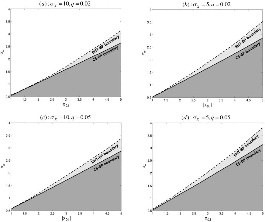
for BHT-BP from (13), respectively. Note that $h_{\text{BHT-BP},i}$ and $h_{\text{CS-BP},i}$ are functions of the noise level $\sigma_{W}$ and square of the signal element $x_{0,i}^{2}$. Therefore, we can ignore the sign of $x_{i,0}$ and handle the signal magnitude $|x_{0,i}|$ in this analysis. The equality condition of (28), and that of (27) divide the plane of $\sigma_{W}$ and $|x_{0,i}|$ into two distinct regions: an ‘SSD-failure’ and an ‘SSD-success’, as depicted in Fig.3. In the figure, the region above the boundary corresponds to $h(\sigma_{W},x_{0,i})\leq 0$, which describes the failure, whereas the region below corresponds to $h(\sigma_{W},x_{0,i})>0$, which describes the success. Such a figure is what we mean by the term PT analysis. Hence, the boundary derived from the equality condition determines the region of success and failure over the plain of $\sigma_{W}$ and $|x_{0,i}|$. The broadness of the success region indicates the recovery ability of the corresponding detector. Namely, the wider the success region is, the more capable a detector is.

The BHT-BP boundary provides a wider success region than the CS-BP boundary does. Examples are shown in Fig.3-(a) for the parameter set $\sigma_{X}=10,q=0.02$, Fig.3-(b) for $\sigma_{X}=5,q=0.02$, Fig.3-(c) for $\sigma_{X}=10,q=0.05$, and Fig.3-(d) for $\sigma_{X}=5,q=0.05$ where we consider the matrix $\mathbf{\Phi}$ with $L=4$. From these examples, it is evident that BHT-BP is superior to CS-BP. In these figures, we also note that BHT-BP generally performs better when the signal magnitude $|x_{0,i}|$ is larger.

Figure 4: Experimental probability of support detection failure for BHT-BP and CS-BP when $N=1024,q=0.02$, and $L=4$.

The result shown in Fig.3 can be interpreted as follows. In the case of CS-BP, additive noise produces the event $\mathcal{F}_{i}$ when the zero-spike becomes the peak of the marginal posterior by exceeding the peak of the slab-PDF, as described in (10). For example, CS-BP misdetects the supportive state with the posteriors of $\sigma_{W}\geq 2$ given in Fig.2. In the BHT-BP case, however, the detector determines the supportive state by considering the noise spreading effect of the posterior, which corresponds to the inner products of the marginal posterior and the function consisting of the prior knowledge, i.e., ${\int{\frac{{f_{X_{i}}(x|S)}}{{f_{X_{i}}(x)}}f_{X_{i}}(x|{\bf{Y}},{\bf{\Phi}})}dx}$, as described in (13). Hence, the detection of BHT-BP is performed by incorporating the posterior function $f_{X_{i}}(x|{\bf{Y}},{\bf{\Phi}})$ over the entire $x$-axis, in contrast to that of CS-BP which only considers the function at a given point. Therefore, BHT-BP detects the signal support against additive noise more robustly than CS-BP does.

Figure 5: Experimental probability of support detection failure for BHT-BP and CS-BP when $N=1024,q=0.05$, and $L=4$.

IV Experimental Results

We support our analytical results with an experimental validation. We measured the probability of the SSD-failure, defined as

$$\Pr\{\mathcal{F}_{i}|S_{i}=1\},$$ (29)

for both BHT-BP and CS-BP over the plain of the noise level $\sigma_{W}$ and signal magnitude $|x_{0,i}|$. For the evaluation of each experimental point, we used the Monte Carlo method with 100 trials where each trial is generated under the parameters of $N=1024,L=4$ and the undersampling ratio $N/M=0.5$. To obtain the marginal posteriors of the signal, we used the iterative BP algorithm introduced in [3],[7],[8].

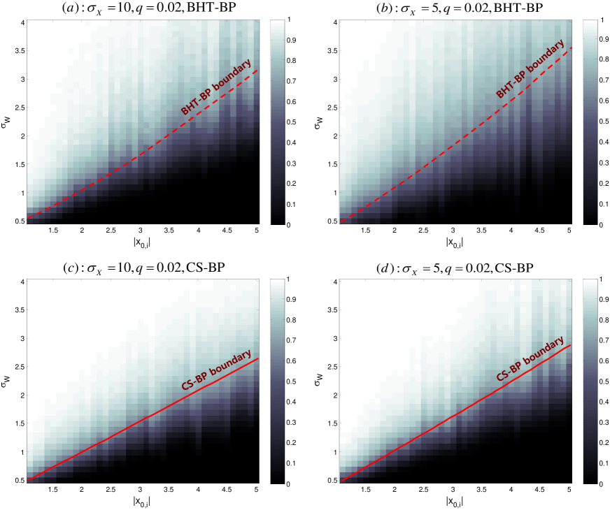
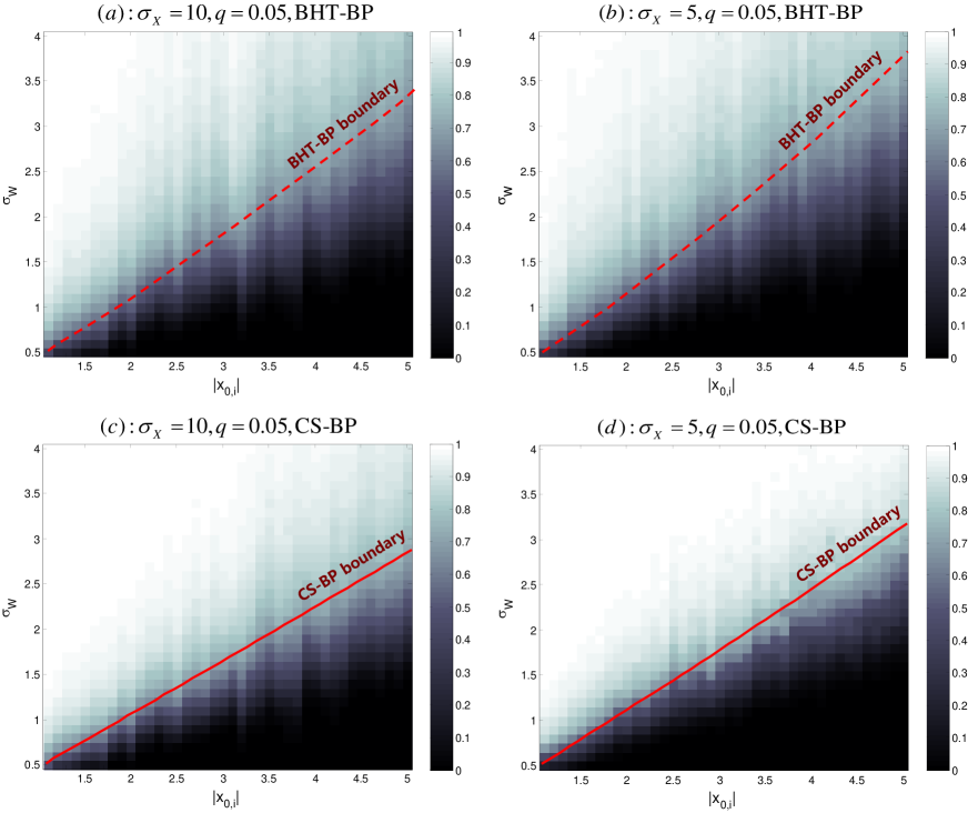
The experimental failure probability of BHT-BP and CS-BP is shown in Fig.4 and Fig.5 for various parameter sets of $(\sigma_{X},q)$, with the corresponding analytical boundary given in Fig.3. In these figures, the brightness of each experimental point represents the value of the failure probability. For example, when the color is bright, the failure probability is close to one. These experimental results show that the figures of CS-BP include a wider white region than that of BHT-BP. We also note in these figures that the transition indeed occurs near the analytical boundary. Thus, we can say that these experimental results are in good agreement with the analytical results given in Section III-B.

V Conclusion

The main aim of this investigation is to answer if a detection oriented algorithm BHT-BP [7],[8] provides any better results than an estimation based algorithm CS-BP [3] for the recovery of sparse support in a noisy underdetermined system of equations. A focus is to come up with a measure with which superiority of one to the other can be made precisely. To this end, we first obtained an expression of the marginal posterior as a function of the noise level and signal magnitude. Using the posterior expression, we have shown that the support detection errors occur only for signal elements on the support. We used such a fact to find the PT boundary which divides the plane of the noise level and signal magnitude into two distinct regions: an “SSD-failure” and an “SSD-succes.” Specifically, the diagram provides information on the required signal magnitude for the recovery under a certain noise level or the allowable noise level for the recovery given a fixed signal magnitude. The PT analysis shows in a clear transition diagram how much BHT-BP is better than CS-BP, in recovering the sparse support.

References

- [1] J. A. Tropp, “Just relax: convex programming methods for identifying sparse signals in noise,” IEEE Trans. Inform. Theory, vol. 52, no. 3, pp. 1030-1051, 2006.
- [2] R. Tibshirani, “Regression shrinkage and selection via the lasso,” J. Roy. Statisti. Soc., Ser. B, vol. 58, no. 1, pp. 267-288, 1996.
- [3] D. Baron, S. Sarvotham, and R. Baraniuk, “Bayesian compressive sensing via belief propagation,” IEEE Trans. Signal Process., vol. 58, no. 1, pp. 269-280, Jan. 2010.
- [4] M. J. Wainwright, “Information-theoretic limits on sparsity recovery in the high-dimensional and noisy setting,” IEEE Trans. Inform. Theory, vol. 55, no. 12, pp. 5728-5741, Dec. 2009.
- [5] M. Akcakaya and V. Tarokh, ”Shannon-theoretic limit on noisy compressive sampling,” IEEE Trans. Inform. Theory, vol. 56, no. 1, pp. 492-504, Jan. 2010.
- [6] A. Fletcher, S. Rangan, and V. Goyal, ”Necessary and sufficient conditions for sparsity pattern recovery,” IEEE Trans. Inform. Theory, vol. 55, no. 12, pp. 5758-5772, Dec. 2009.
- [7] J. Kang, H.-N. Lee, and K. Kim, “Bayesian hypothesis test for sparse support recovery using belief propagation,” Proc. in IEEE Statistical Signal Processing Workshop (SSP), pp. 45-48, Aug. 2012.
- [8] J. Kang, H.-N. Lee, and K. Kim, “Detection-Directed sparse estimation using Bayesian hypothesis test and belief propagation,” 2012 [Online]. Available: arXiv:1211.1250 [cs.IT].
- [9] D. L. Donoho and J. Tanner, “Neighborliness of randomly projected simplices in high dimensions,” Proc. Nat. Acad. Sci. USA, vol. 102, no. 27, pp. 9452-9457, 2005.
- [10] D. L. Donoho and J. Tanner, “Precise undersampling theorems,” Proceeding of the IEEE, vol. 98, issue 6, pp. 913-924, June, 2010.
- [11] D. Guo and S. Verdu, “Randomly spread CDMA: Asymptotics via statistical physics,” IEEE Trans. Inform. Theory, vol. 51, no. 6, pp. 1983-2010, Jun. 2005.
- [12] D. Guo and C.-C. Wang, “Random sparse linear systems observed via arbitrary channels: a decoupling principle,”Proc. in IEEE Int. Symp. Inform. Theory (ISIT), pp. 946-950, Nice, France, June. 2007.
- [13] D. Guo and C.-C. Wang, “Asymptotic mean-square optimality of belief propagation for sparse linear systems,” Proc. in IEEE Inform. Theory Workshop (ITW), pp. 194-198, Chengdu, China, Oct. 2006.
- [14] D. L. Donoho, M. Elad, and V. Temlyakov, “Stable recovery of sparse overcomplete representations in the presence of noise,” IEEE Trans. Inform. Theory, vol. 52, no. 1, pp. 6-18, Jan. 2006.