Convergence to the Tracy-Widom distribution for longest paths in a directed random graph
Abstract.
We consider a directed graph on the 2-dimensional integer lattice, placing a directed edge from vertex to , whenever , , with probability , independently for each such pair of vertices. Let denote the maximum length of all paths contained in an rectangle. We show that there is a positive exponent , such that, if , as , then a properly centered/rescaled version of converges weakly to the Tracy-Widom distribution. A generalization to graphs with non-constant probabilities is also discussed.
Key words and phrases:
Random graph, last passage percolation, strong approximation, Tracy-Widom distribution.2000 Mathematics Subject Classification:
Primary 05C80, 60F05; secondary 60K35, 06A06.1. Introduction
Random directed graphs form a class of stochastic models with applications in computer science (Isopi and Newman, 1994), biology (Cohen and Newman, 1991; Newman, 1992; Newman and Cohen, 1986) and physics (Itoh and Krapivsky, 2012). Perhaps the simplest of all such graphs is a directed version of the standard Erdős-Rényi random graph (Barak and Erdős, 1984) on vertices, defined as follows: For each pair of distinct positive integers less than , toss a coin with probability of head equal to , , independently from pair to pair; if head shows up then introduce an edge directed from to . There is a natural extension of this graph to the whole of studied in detail in Foss and Konstantopoulos (2003). In particular, if we define the asymptotic growth rate , as the a.s. limit of the maximum length of all paths between and divided by , Foss and Konstantopoulos (2003) provide sharp bounds on for all values of .
A natural generalization arises when we replace the total order of the vertex set by a partial order, usually implied by the structure of the vertex set. In such a model, coins are tossed only for pairs of vertices which are comparable in this partial order. The canonical case is to consider, as a vertex set, the 2-dimensional integer lattice , equipped with the standard component-wise partial order: if the two pairs are distinct and , . Such a graph was considered in Denisov et al. (2012). In that paper, it was shown that if denotes the maximum length of all paths of the graph, restricted to , then there is a positive (depending on and the fixed integer ), such that
| (1.1) |
where is the stochastic process defined in terms of independent standard Brownian motions, , via the formula
One can speak of as a Brownian directed percolation model, the terminology stemming from the picture of a “weighted graph” on where the weight of a segment equals the change of a Brownian motion. If a path from to is defined as a union of such segments, then represents the maximum weight of all such paths.
Baryshnikov (2001), answering an open question by Glynn and Whitt (1991), showed that
where is the largest eigenvalue of a GUE matrix of dimension . Since is -self-similar, we see that
Now, fluctuations of around the centering sequence have been quantified by Tracy and Widom (1994) who showed the existence of a limiting law, denoted by :
A natural question then, raised in Denisov et al. (2012), is whether one can obtain as a weak limit of when and tend to infinity simultaneously. Our paper is concerned with resolving this question. To see what scaling we can expect, rewrite the last display, for arbitrary , as
A statement of the form , where the distribution of does not depend on the choice of , implies the statement , for any function such that . Hence, upon setting , we have
| (1.2) |
Therefore, it is reasonable to guess that, when is small enough, an analogous limit theorem holds for a centered scaled version of the largest length , namely that
| (1.3) |
where are appropriate constants.
A stochastic model, bearing some resemblance to ours, is the so-called directed last passage percolation model on (the case being of interest here). We are given a collection of i.i.d. random variables indexed by elements of . A path from the origin to the point is a sequence of elements of , starting from the origin and ending at , such that the difference of successive members of the sequence is equal to the unit vector in the th direction, for some . The weight of a path is the sum of the random variables associated with its members. Specializing to , let be the largest weight of all paths from to . Assuming that the random variables have a finite moment of order larger than , Bodineau and Martin (2005) showed that (1.3) holds for all sufficiently small positive (the threshold depending on the order of the finite moment). Independently, Baik and Suidan (2005) obtained the same result for random variables with a finite th moment and for . In both papers, partial sums of i.i.d. were approximated with Brownian motions, in the first case using the Komlós-Major-Tusnády (KMT) construction, while in the second using Skorokhod embedding.
To show that (1.3) holds for our model, we adopt the technique introduced in Denisov et al. (2012), which involves the existence of skeleton points on each line . Skeleton points are, by definition, random points which are connected with all the other points on the same line. In Denisov et al. (2012) Denisov, Foss and Konstantopoulos used this fact, together with the fact that, for finite , one can pick skeleton points common to all lines, in order to prove (1.1). However, when tends to infinity simultaneously with , it is not possible to pick skeleton points common to all lines. Modifying the definition of skeleton points enables us to give a new proof of (1.1), as well as to prove (1.3). To achieve the latter, we borrow the idea of KMT coupling from Bodineau and Martin (2005). However, we need to do some work in order to express the random variable in a way that resembles a maximum of partial sums.
Although we focus on the case where the edge probability is constant, it is possible to consider a more general case, where the probability that a vertex connects to a vertex depends on the distances and of the two vertices. This generalization is discussed in the last section of the article.
2. The one-dimensional directed random graph
We summarize below some properties of the directed Erdős-Rényi graph on with connectivity probability taken from Foss and Konstantopoulos (2003). For , let be the maximum length of all paths with start and end points in the interval . Then, for , we have . Since the distribution of the random graph is invariant under translations, and is also ergodic (the natural invariant -field is trivial), it follows, from Kingman’s subadditive ergodic theorem, that there is a deterministic constant such that
| (2.1) |
In fact, . The function is not known explicitly; only bounds are known (Foss and Konstantopoulos, 2003, Thm. 10.1). For example, . We also know that there exists, almost surely, a random integer sequence with the property that for all , all , and all , there is a path from to and a path from to . The existence of such points, referred to as skeleton points, is not hard to establish (Denisov et al., 2012). Since the directed Erdős-Rényi graph is invariant under translations, so is the sequence of skeleton points, i.e., has the same law as , for all . Moreover, it turns out that the sequence forms a stationary renewal process. If we enumerate the skeleton points according to , we have that are independent random variables, whereas are i.i.d. Stationarity implies that the law of the omitted difference has a density which is proportional to the tail of the distribution of . In Denisov et al. (2012) it is shown that the distance between two successive skeleton points has a finite nd moment. One can follow the same steps of the proof, to show that in our case, with constant probability , this random variable has moments of all orders. Moreover, one can show that for some (the maximal such depends on ) it holds that .
The rate of the sequence of skeleton points can be expressed as an infinite product:
| (2.2) |
For example, for , .
A central limit theorem for is also available (Denisov et al., 2012, Thm. 2). If we let
| (2.3) |
then
| (2.4) |
where is a standard normal random variable. Note that . Unfortunately, we have no estimates for , but, interestingly, there is a technique for estimating it, based on perfect simulation. This was briefly explained in Foss and Konstantopoulos (2003) in connection with an infinite-dimensional Markov chain which carries most of the information about the law of the directed Erdős-Rényi random graph.
In addition, it is shown in Foss and Konstantopoulos (2003) that can also be expressed as
| (2.5) |
In fact, if is a random sequence of integers, defined on the same probability space as the one supporting the random graph, such that is a stationary point process then
The most important property of the skeleton points is that if is a skeleton point, and if , then a path with length (a maximum length path) must necessarily contain . This crucial property will be used several times below, especially since, for every , the following equality holds
Furthermore, the restriction of the graph on the interval between two successive skeleton points is independent of the restriction on the complement of the interval; hence the summands in the right-hand side of the last display are independent random variables.
3. Statement of the main result
It is clear from (2.4) that the constants in (1.3) should be as follows: , . Now we can formulate the main result.
Theorem 3.1.
Let , , be the quantities associated with the directed random graph on with connectivity probability , defined by (2.1) (equivalently, (2.5)), (2.2), (2.3), respectively. Consider the directed random graph on and let be the maximum length of all paths between two vertices in . Then, for all ,
| (3.1) |
where is the Tracy-Widom distribution.
To prove this theorem, we will first define the notion of skeleton points for the graph on and then prove pathwise upper and lower bounds for which depend on paths going through these skeleton points. This will be done in Section 4. In Section 5.1 we show that the difference between these bounds is of the order , where is the net exponent in the denominator of (3.1). We will then (Section 5.2) introduce a quantity which resembles a last passage percolation problem and show that it differs from by a quantity which is of the order , when . The problem will then be translated to a last passage percolation problem (with the exception of random indices). This will finally, in Section 5.3 be compared to the Brownian directed percolation problem by means of strong coupling.
4. Skeleton points and pathwise bounds
Our model is a directed random graph with vertices . For each pair of vertices , , such that , toss an independent coin with probability of heads equal to ; if a head shows up introduce an edge directed from to .
A path of length in the graph is a sequence of vertices such that there is an edge between any consecutive vertices.
We denote by the restriction of on the set of vertices . The random variable of interest is
We refer to the set as “line ” or “th line”, and note that the restriction of onto is a directed Erdős-Rényi random graph. We denote this restriction by . Typically, a superscript will refer to a quantity associated with this restriction. For example, for ,
| the maximum length of all paths in | |||
| with vertices between and |
and we agree that if .
Clearly, the are i.i.d. random graphs, identical in distribution to the directed Erdős-Rényi random graph. Therefore, for each ,
To establish upper and lower bounds for , we need to slightly change the definition of a skeleton point in .
Definition 4.1 (Skeleton points in ).
A vertex of the directed random graph is called skeleton point if it is a skeleton point for (for any , there is a path from to and a path from to ) and if there is an edge from to .
Therefore, the skeleton points on line are obtained from the skeleton point sequence of the directed Erdős-Rényi random graph by independent thinning with probability . When we refer to skeleton points on line , we shall be speaking of this thinned sequence. The elements of this sequence are denoted by
and have rate
The associated counting process of skeleton points on line is defined by
together with the agreement that
Note that we insist on having the parameter in as an element of (and not just ). We also let
be the skeleton points on line straddling :
| (4.1) |
Next we prove upper and lower bounds for . The set of dissections of the interval in non-overlapping, possibly empty intervals is denoted by
Lemma 4.2.
(Upper bound) Define
| (4.2) |
Then .
Proof.
Let be a path in . Consider the lines visited by , denoting their indices by . Let and be the first and the last vertex of line in the path . Then the length of satisfies
Since successive vertices in the path should be increasing in the order , we have , . Hence, with ,
where we used (4.1). Since , we can extend to a dissection of into non-overlapping intervals, showing that the right-hand side of the last display is bounded above by . Taking the maximum over all in , we obtain , as required. ∎
Note that the existence and properties of skeleton points were not used in the proof of the upper bound, other than to ensure that the upper bound is a.s. finite.
Lemma 4.3.
(Lower bound) Define
and
Then .
Proof.
We will show that, for all , there is a path in with length satisfying
| (4.3) |
Fix and use the notation
Note that if there is one or no skeleton points on the segment and then .
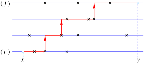
Given two skeleton points , we say that there is a staircase path from to if there is a sequence of skeleton points
such that . See Figure 4.1. Clearly then, there is a path from to which jumps upwards by one step each time it meets a new skeleton point from the sequence. We denote this by
Among all the staircase paths from to , we will consider the best one, defined by two properties:
-
•
Property 1: A best path from to jumps from line to line , , at the first next skeleton point on line , i.e. at the points and
-
•
Property 2: Every horizontal segment of a best path is a path of maximal length.
If all the intervals are empty, the left-hand side of (4.3) is zero and the inequality is trivially satisfied for any path .
Otherwise, for a fixed we will construct a path in for which (4.3) holds. Define a subsequence of , inductively, as follows:
| (4.4) | ||||
| (4.5) |
See Figure 4.2 for an illustration. The procedure stops if one of the elements of the subsequence exceeds or if the condition inside the infimum is not satisfied by a path in .
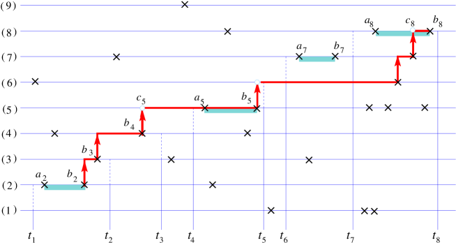
Let be the last index in the above defined sequence. Let be a path of maximum length from to and define, for , a path as a best staircase path from to . Note that, for each , , the end vertex of is the start vertex of . Therefore we can concatenate the paths to obtain a path . This path starts from and ends at .
Let
and its length on line . Also, for denote
| the first vertex on line of path . |
Split the sum in the left-hand side of (4.3) along the elements of the subsequence :
where we have conveniently set
| , , |
in order to take care of the first and last terms. By the defintion of , the intervals are empty and
Assume now that , and write
Since is the path of maximal length from to its end-vertex (Property 2), if then . Define in this case . Otherwise, we can write
Then, again because of Property 2, and it is left to find a bound on the interval . Recall that by Property 1, depending whether is a member of the sequence or not, or , respectively. Also, because of , we know that . Hence, if it holds
Combining the above, we obtain
If , then . Otherwise, we can extend the sequence defining iteratively and until for some . Let be the last index such that . As there was not possible to construct the best staircase path after the line , is at most . Similarly as above, for it holds
Finally, we obtain
as required. ∎
5. Further estimates in probability and Brownian directed percolation
In the present section we prove Theorem 3.1 as a sequence of lemmas.
5.1. Asymptotic coincidence of the two bounds
Looking at (1.3), we can see that the correct scaling requires exponent
in the denominator and condition , which is equivalent to .
In the following two lemmas we will not specifically use the definiton of and condition on . Both lemmas hold for more general , .
Lemma 5.1.
With and ,
5.2. Centering
We introduce the quantity
This should be “comparable” to when . Indeed, we have:
Lemma 5.2.
With , and ,
Proof.
We begin by rewriting the numerator above as
Upon writing , for any , we have
Hence, on the one hand we have
On the other hand,
Therefore,
Thus, for , the result follows by applying Lemma A.1 and Lemma 5.1. ∎
Define now variance as
and observe that . We work with the quantity , which can be rewritten as
where
Note that the random variables , indexed by both and , are independent and that are identically distributed with zero mean and unit variance. The fact that the do not have the same distribution will not affect the result, so we will not separately take care of it.
5.3. Coupling with Brownian motion
The term resembles a centered last passage percolation path weight, except that random indices are involved. Therefore, we start using the idea of strong coupling with Brownian motions, analogously to the proof in Bodineau and Martin (2005). Let be i.i.d. standard Brownian motions, and recall that
| (5.1) |
Define the random walks by
| (5.2) |
with . With this notation, we have
| (5.3) |
Taking into account (1.2) and Lemma 5.2, it is evident that to prove Theorem 3.1 it remains to show that
or, using the scaling property of Brownian motion, that:
Lemma 5.3.
For all ,
To show that the random walks are close enough to the Brownian motion we use the following version of the Komlós-Major-Tusnády strong approximation result (Komlós et al., 1976, Thm. 4):
Theorem 5.4.
For any , and , starting with a probability space supporting independent Brownian motions , , we can jointly construct i.i.d. sequences , , with the correct distributions and, moreover, such that, with as in (5.2) above,
where the constants are depending on , and distributions of and .
In addition to this, in order to take care of the random indices appearing in (5.3), we need a convergence rate result for the counting processes which is proven in the appendix.
Proof of Lemma 5.3.
where
Therefore, it is enough to show that,
For the first convergence we will take into account the coupling estimate as in Theorem 5.4. That is, we will throughout assume that the random walks and Brownian motions have been constructed jointly. The second convergence will be established without this estimate, i.e., we will show that it is true, regardless of the joint construction of the Brownian motions and the random walks. This is because the coupling we use is not detailed enough to give us information about the joint distribution of and the counting process (the latter is not a function of the random walks used in the coupling).
Proof of the first convergence. Let . We need to show that
Let . Then
| (5.4) |
The first term from right-hand side is zero for large . We are allowed, for large enough, to estimate the second term using Theorem 5.4 for an arbitrary and as
as .
Proof of the second convergence. Let . Replacing by in (5.4), we see that the first term is again zero for large and it remains to show that second term converge to 0, i.e., it is enough to show the convergence for its upper-bound
as . Let and . Then we can write
Corollary A.1 implies the convergence of the first term above
as , where . Set . For the second term using the fact that, under our condition, for , we have
| (a) | |||
| (b) |
as . The inequality (a) is the consequence of and the inequality (b) is an estimate for the tail of the normal distribution. ∎
Remark 5.5.
The condition is equivalent to and, thus, it ensures existence of an and later existance of . Therefore, it is necessary for application of Lemma A.1, as well as for the convergence of the last estimate above.
6. Graph with non-constant edge probabilities
In Denisov et al. (2012), the authors consider a one-dimensional model with connectivity probabilities depending on the distance between points, i.e. there is an edge between the vertices and with probability . To prove a central limit theorem for the maximal path length in that graph, two conditions are introduced:
-
•
;
-
•
.
The conditions guarantee the existence of skeleton points and finite variance, defined as in (2.3).
We can extend the idea of the graph on keeping, whenever possible, the notation from the graph with constant probability .
Let be a sequence of probabilities that satisfies the following:
-
•
;
-
•
;
-
•
for some .
Then the vertices and , , are connected with probability .
The conditions above are needed to ensure the existence of skeleton points, as in Definition 4.1, and a finite th moment of the random variables for some .
From now on, let denote the order of the highest finite moment, i.e.
Now we can state the analogue of Theorem 3.1 for this more general setting:
Theorem 6.1.
For all ,
Proof.
We follow the lines of the proof of Theorem 3.1, emphasizing the points one should be careful about or which need to be modified.
The construction of the upper and lower bounds for is the same as in Section 4. In Lemma 5.1 and Lemma 5.2, the term converges to 0 if , which leads to the constraint .
Proof of the first convergence. Instead of Theorem 5.4, we use the combination of results from Komlós et al. (1976) and Major (1976), as stated in Proposition 2 of Bodineau and Martin (2005), which allow us to couple Brownian motions , and random walks , so that
| (6.1) |
Let . We want to establish convergence of the same terms as in (5.4). Applying, on the first term, the Markov inequality and properties of the coupling with Brownian motion (6.1) yield:
as . For the second term we use again the coupling properties (6.1):
as because due to our new constraint on .
Proof of the second convergence. Here, the only change is the replacement of Lemma A.2 by part of Theorem 6.12.1 in Gut (2013), in our notation:
If , then for all it holds that as .
One can, in the same fashion as before, prove the following analogue of Corollary A.1,
Likewise in Remark 5.5, condition is necessary. Another constraint that occurs is and it can be shown that this is satisfied if . ∎
Appendix A
Lemma A.1.
Let and be a sequence of non-negative i.i.d. random variables such that Then,
Proof.
It suffices to prove the lemma for , since then the result for follows easily by Jensen’s inequality. Let and . Borel-Cantelli lemma, together with the assumption , give , almost surely, as . An easy computation shows that then also , almost surely, as .
On the other hand, we know that for all and that is uniformly integrable. Therefore, is also unformly integrable and as (Gut, 2013, Thm. 5.4.5, Thm. 5.5.2). ∎
The following lemma is an analogue of a result by (Lanzinger, 1998, Prop. 2), with slight improvement in the probability bound. Moreover, we specialize the lemma to our case.
Lemma A.2.
Let and . Suppose that are i.i.d. random variables such that and for some , and set . Then, for all ,
as .
Proof.
Without loss of generality we can assume that . We first show that, for all , as .
For fixed , define and set . Note that and that for , where and , it holds that . We can write
| (A.1) |
We first find a bound for the moment generating function for in :
where for the first inequality we used and for the last one . Now, using Markov’s inequality and the bound above for the first term in (A.1) yields
For the second term in (A.1), again using Markov’s inequality, we have
Combining the two estimates finally establishes that
as because of the choice of and .
By symmetry, the same convergence rate holds also for .
Thus, the statement of the theorem follows using Lévy inequality (Gut, 2013, Thm. 3.7.2) and the fact that for large enough we can find such that :
Corollary A.1.
Let be positive, integer-valued i.i.d. random variables and suppose that the assumptions of Lemma A.2 are satisfied. Then, for the counting process , where , it holds that
Proof.
For the counting process we have . Therefore, we can write
where . Thus,
The first and the second term above converge to 0 as by Lemma A.2. We prove convergence to 0 for the third term using Markov’s inequality,
Acknowledgements
We thank Allan Gut and Svante Janson for valuable comments.
References
- Baik and Suidan (2005) J. Baik and T. M. Suidan. A GUE central limit theorem and universality of directed first and last passage site percolation. Int. Math. Res. Not. 2005 (6), 325–337 (2005). MR2131383.
- Barak and Erdős (1984) A. B. Barak and P. Erdős. On the maximal number of strongly independent vertices in a random acyclic directed graph. SIAM J. Algebr. Discr. Methods 5 (4), 508–514 (1984). MR0763980.
- Baryshnikov (2001) Y. Baryshnikov. GUEs and queues. Probab. Theory Related Fields 119 (2), 256–274 (2001). MR1818248.
- Bodineau and Martin (2005) T. Bodineau and J. Martin. A universality property for last-passage percolation paths close to the axis. Electron. Commun. Probab. 10, 105–112 (2005). MR2150699.
- Cohen and Newman (1991) J. E. Cohen and C. M. Newman. Community area and food-chain length: theoretical predictions. Amer. Naturalist 138 (6), 1542–1554 (1991). www.jstor.org/stable/2462559.
- Denisov et al. (2012) D. Denisov, S. Foss and T. Konstantopoulos. Limit theorems for a random directed slab graph. Ann. Appl. Probab. 22 (2), 702–733 (2012). MR2953567.
- Foss and Konstantopoulos (2003) S. Foss and T. Konstantopoulos. Extended renovation theory and limit theorems for stochastic ordered graphs. Markov Process. Related Fields 9 (3), 413–468 (2003). MR2028221.
- Glynn and Whitt (1991) P. W. Glynn and W. Whitt. Departures from many queues in series. Ann. Appl. Probab. 1 (4), 546–572 (1991). MR1129774.
- Gut (2013) A. Gut. Probability: A Graduate Course. Springer, New York, 2nd edition (2013). MR2977961.
- Isopi and Newman (1994) M. Isopi and C. M. Newman. Speed of parallel processing for random task graphs. Comm. Pure and Appl. Math 47 (3), 361–376 (1994). MR1266246.
- Itoh and Krapivsky (2012) Y. Itoh and P. L. Krapivsky. Continuum cascade model of directed random graphs: traveling wave analysis. J. Phys. A 45 (45) (2012). MR2990512.
- Komlós et al. (1976) J. Komlós, P. Major and G. Tusnády. An approximation of partial sums of independent RV’s, and the sample DF. II. Z. Wahrsch. und Verw. Gebiete 34 (1), 33–58 (1976). MR0402883.
- Lanzinger (1998) H. Lanzinger. A Baum-Katz theorem for random variables under exponential moment conditions. Statist. Probab. Lett. 39 (2), 89–95 (1998). MR1652524.
- Major (1976) P. Major. The approximation of partial sums of independent RV’s. Z. Wahrsch. und Verw. Gebiete 35 (3), 213–220 (1976). MR0415743.
- Newman (1992) C. M. Newman. Chain lengths in certain random directed graphs. Random Structures Algorithms 3 (3), 243–253 (1992). MR1164838.
- Newman and Cohen (1986) C. M. Newman and J. E. Cohen. A stochastic theory of community food webs IV: Theory of food chains in large webs. Proc. R. Soc. London Ser. B 228 (1252), 355–377 (1986). www.jstor.org/stable/36124.
- Tracy and Widom (1994) C. A. Tracy and H. Widom. Level-spacing distributions and the Airy kernel. Comm. Math. Phys. 159 (1), 151–174 (1994). MR1257246.