Stochastic filtering via $L^{2}$ projection on mixture manifolds with computer algorithms and numerical examples
Updated version in Mathematics of Control, Signals & Systems 28(1), 1-33, 2016

Abstract

We examine some differential geometric approaches to finding approximate solutions to the continuous time nonlinear filtering problem. Our primary focus is a new projection method for the optimal filter infinite dimensional Stochastic Partial Differential Equation (SPDE), based on the direct L2 metric and on a family of normal mixtures. We compare this method to earlier projection methods based on the Hellinger distance/Fisher metric and exponential families, and we compare the L2 mixture projection filter with a particle method with the same number of parameters, using the Levy metric. We prove that for a simple choice of the mixture manifold the L2 mixture projection filter coincides with a Galerkin method, whereas for more general mixture manifolds the equivalence does not hold and the L2 mixture filter is more general. We study particular systems that may illustrate the advantages of this new filter over other algorithms when comparing outputs with the optimal filter. We finally consider a specific software design that is suited for a numerically efficient implementation of this filter and provide numerical examples.

Keywords: Direct L2 metric, Exponential Families, Finite Dimensional Families of Probability Distributions, Fisher information metric, Hellinger distance, Levy Metric, Mixture Families, Stochastic filtering, Galerkin

AMS Classification codes: 53B25, 53B50, 60G35, 62E17, 62M20, 93E11

1 Introduction

In the nonlinear filtering problem one observes a system whose state is known to follow a given stochastic differential equation. The observations that have been made contain an additional noise term, so one cannot hope to know the true state of the system. However, one can reasonably ask what is the probability density over the possible states.

When the observations are made in continuous time, the probability density follows a stochastic partial differential equation known as the Kushner–Stratonovich equation. This can be seen as a generalization of the Fokker–Planck equation that expresses the evolution of the density of a diffusion process. Thus the problem we wish to address boils down to finding approximate solutions to the Kushner–Stratonovich equation.

For a quick introduction to the filtering problem see Davis and Marcus (1981) [19]. For a more complete treatment from a mathematical point of view see Lipster and Shiryayev (1978) [34] and Bain and Crisan [8]. See Jazwinski (1970) [26] and Ahmed (1998) [2] for a comprehensive treatment of filtering. For recent results see the volume [16].

The main idea we will employ is inspired by the differential geometric approach to statistics developed in [3] and [38]. The idea of applying this approach to the filtering problem has been sketched first in [22]. One thinks of the probability distribution as evolving in an infinite dimensional space ${\cal P}$ which is in turn contained in some Hilbert space $H$. One can then think of the Kushner–Stratonovich equation as defining a vector field in ${\cal P}$: the integral curves of the vector field should correspond to the solutions of the equation. To find approximate solutions to the Kushner–Stratonovich equation one chooses a finite dimensional submanifold $M$ of $H$ and approximates the probability distributions as points in $M$. At each point of $M$ one can use the Hilbert space structure to project the vector field onto the tangent space of $M$. One can now attempt to find approximate solutions to the Kushner–Stratonovich equations by integrating this vector field on the manifold $M$.

This mental image is slightly innaccurate. The Kushner–Stratonovich equation is a stochastic PDE rather than a PDE so one should imagine some kind of stochastic vector field rather than a smooth vector field. Thus in this approach we hope to approximate the infinite dimensional stochastic PDE by solving a finite dimensional stochastic ODE on the manifold.

Note that our approximation will depend upon two choices: the choice of manifold $M$ and the choice of Hilbert space structure $H$. In this paper we will consider two possible choices for the Hilbert space structure: the direct $L^{2}$ metric on the space of probability distributions; the Hilbert space structure associated with the Hellinger distance and the Fisher Information metric. Our focus will be on the direct $L^{2}$ metric since projection using the Hellinger distance has been considered before. As we shall see, the choice of the “best” Hilbert space structure is determined by the manifold one wishes to consider — for manifolds associated with exponential families of distributions the Hellinger metric leads to the simplest equations, whereas the direct $L^{2}$ metric works well with mixture distributions.

It was proven in [13] that the projection filter in Hellinger metric on exponential families is equivalent to the classical assumed density filters. In this paper, we show that the projection filter for basic mixture manifolds in L2 metric is equivalent to a Galerkin method. This only holds for very basic mixture families, however, and the L2 projection method turns out to be more general than the Galerkin method.

We will write down the stochastic ODE determined by the geometric approach when $H=L^{2}$ and show how it leads to a numerical scheme for finding approximate solutions to the Kushner–Stratonovich equations in terms of a mixture of normal distributions. We will call this scheme the $L^{2}$ normal mixture projection filter or simply the L2NM projection filter.

The stochastic ODE for the Hellinger metric was considered in [14], [12] and [13]. In particular a precise numerical scheme is given in [14] for finding solutions by projecting onto an exponential family of distributions. We will call this scheme the Hellinger exponential projection filter or simply the HE projection filter.

En passant, we clarify why we use the Kushner–Stratonovich and not the alternative Duncan–Mortensen–Zakai (Zakai for brevity) equation for nonlinear filtering. The Zakai equation is the preferred stochastic partial differential equation in nonlinear filtering [2], since it is a linear equation and admits a robust version. It models a particular unnormalized version of the optimal filter density. We will show that projecting the Zakai equation in Hellinger metric results in the same approximate filter as projecting the Zakai equation. Intuitively, in Hellinger metric square roots of densities are part of the unit sphere in $L^{2}$ and re-scaling is orthogonal to the tangent space. Thus in Hellinger metric we could indeed use the Zakai equation and we would obtain the same filter. However, when projecting according to the direct metric, this no longer holds and projecting the Zakai equation would lead to a different filter than projecting the Kushner Stratonovich equation. Since we are interested in approximating well the density and not an unnormalized version of it, we use the Kushner–Stratonovich equation throughout the paper.

We will compare the results of a C++ implementation of the L2NM projection filter with a number of other numerical approaches including the HE projection filter and the optimal filter. We can measure the goodness of our filtering approximations thanks to the geometric structure and, in particular, the precise metrics we are using on the spaces of probability measures.

What emerges is that the two projection methods produce excellent results for a variety of filtering problems. The results appear similar for both projection methods; which gives more accurate results depends upon the problem.

As we shall see, however, the L2NM projection approach can be implemented more efficiently. In particular one needs to perform numerical integration as part of the HE projection filter algorithm whereas all integrals that occur in the L2NM projection can be evaluated analytically.

We also compare the L2NM filter to a particle filter with the best possible combination of particles with respect to the Lévy metric. Introducing the Lévy metric is needed because particles densities do not compare well with smooth densities when using $L^{2}$ induced metrics. We show that, given the same number of parameters, the L2NM may outperform a particles based system.

The paper is structured as follows: In Section 2 we introduce the nonlinear filtering problem and the infinite-dimensional Stochastic PDE (SPDE) that solves it. In Section 3 we introduce the geometric structure we need to project the filtering SPDE onto a finite dimensional manifold of probability densities. In Section 4 we perform the projection of the filtering SPDE according to the L2NM framework and also recall the HE based framework. In Section 5 we prove equivalence between the projection filter in L2 metric for basic mixture families and the Galerkin method. In Section 6 we briefly introduce the main issues in the numerical implementation and then focus on software design for the L2NM filter. In Section 7 a second theoretical result is provided, showing a particularly convenient structure for the projection filter equations for specific choices of the system properties and of the mixture manifold.

In Section 8 we look at numerical results, whereas in Section 9 we compare our outputs with a particle method. Section 10 concludes the paper.

2 The non-linear filtering problem with
continuous-time observations

In the non-linear filtering problem the state of some system is modelled by a process $X$ called the signal. This signal evolves over time $t$ according to an Itô stochastic differential equation (SDE). We measure the state of the system using some observation $Y$. The observations are not accurate, there is a noise term. So the observation $Y$ is related to the signal $X$ by a second equation.

$$\begin{array}[]{rcl}dX_{t}&=&f_{t}(X_{t})\,dt+\sigma_{t}(X_{t})\,dW_{t},\ \ X_{0},\\ \\ dY_{t}&=&b_{t}(X_{t})\,dt+dV_{t},\ \ Y_{0}=0\ .\end{array}$$ (1)

In these equations the unobserved state process $\{X_{t},t\geq 0\}$ takes values in ${\mathbb{R}}^{n}$, the observation $\{Y_{t},t\geq 0\}$ takes values in ${\mathbb{R}}^{d}$ and the noise processes $\{W_{t},t\geq 0\}$ and $\{V_{t},t\geq 0\}$ are two Brownian motions.

The nonlinear filtering problem consists in finding the conditional probability distribution $\pi_{t}$ of the state $X_{t}$ given the observations up to time $t$ and the prior distribution $\pi_{0}$ for $X_{0}$.

Let us assume that $X_{0}$, and the two Brownian motions are independent. Let us also assume that the covariance matrix for $V_{t}$ is invertible. We can then assume without any further loss of generality that its covariance matrix is the identity. We introduce a variable $a_{t}$ defined by:

$$a_{t}=\sigma_{t}\sigma_{t}^{T}$$

With these preliminaries, and a number of rather more technical conditions which we will state shortly, one can show that $\pi_{t}$ satisfies the a stochastic PDE called the Kushner–Stratonovich equation. This states that for any compactly supported test function $\phi$ defined on ${\mathbb{R}}^{n}$

$$\pi_{t}(\phi)=\pi_{0}(\phi)+\int_{0}^{t}\pi_{s}({\cal L}_{s}\phi)\,ds+\sum_{k=1}^{d}\int_{0}^{t}[\pi_{s}(b_{s}^{k}\,\phi)-\pi_{s}(b_{s}^{k})\,\pi_{s}(\phi)]\,[dY_{s}^{k}-\pi_{s}(b_{s}^{k})\,ds]\ ,$$ (2)

where for all $t\geq 0$, the backward diffusion operator ${\cal L}_{t}$ is defined by

$${\cal L}_{t}=\sum_{i=1}^{n}f_{t}^{i}\,\frac{\partial}{\partial x_{i}}+{\textstyle\frac{1}{2}}\sum_{i,j=1}^{n}a_{t}^{ij}\,\frac{\partial^{2}}{\partial x_{i}\partial x_{j}}\ .$$

Equation (2) involves the derivatives of the test function ${\phi}$ because of the expression ${\cal L}_{s}\phi$. We assume now that $\pi_{t}$ can be represented by a density $p_{t}$ with respect to the Lebesgue measure on ${\mathbb{R}}^{n}$ for all time $t\geq 0$ and that we can replace the term involving ${\cal L}_{s}\phi$ with a term involving its formal adjoint ${\cal L}^{*}$. Thus, proceeding formally, we find that $p_{t}$ obeys the following Itô-type stochastic partial differential equation (SPDE):

$${\mathrm{d}}p_{t}={\cal L}^{*}_{t}p_{t}{\mathrm{d}}t+\sum_{k=1}^{d}p_{t}[b_{t}^{k}-E_{p_{t}}\{b_{t}^{k}\}][{\mathrm{d}}Y_{t}^{k}-E_{p_{t}}\{b_{t}^{k}\}{\mathrm{d}}t]$$

where $E_{p_{t}}\{\cdot\}$ denotes the expectation with respect to the probability density $p_{t}$ (equivalently the conditional expectation given the observations up to time $t$). The forward diffusion operator ${\cal L}^{*}_{t}$ is defined by:

$${\cal L}_{t}^{*}\phi=-\sum_{i=1}^{n}\frac{\partial}{\partial x_{i}}[f_{t}^{i}\phi]+{\textstyle\frac{1}{2}}\sum_{i,j=1}^{n}\frac{\partial^{2}}{\partial x_{i}\partial x_{j}}[a_{t}^{ij}\phi].$$

This equation is written in Itô form. When working with stochastic calculus on manifolds it is necessary to use Stratonovich SDE’s rather than Itô SDE’s. This is because one does not in general know how to interpret the second order terms that arise in Itô calculus in terms of manifolds. The interested reader should consult [20]. A straightforward calculation yields the following Stratonvich SPDE:

$$dp_{t}={\cal L}_{t}^{\ast}\,p_{t}\,dt-{\textstyle\frac{1}{2}}\,p_{t}\,[|b_{t}|^{2}-E_{p_{t}}\{|b_{t}|^{2}\}]\,dt+\sum_{k=1}^{d}p_{t}\,[b_{t}^{k}-E_{p_{t}}\{b_{t}^{k}\}]\circ dY_{t}^{k}\ .$$

We have indicated that this is the Stratonovich form of the equation by the presence of the symbol ‘$\circ$’ inbetween the diffusion coefficient and the Brownian motion of the SDE. We shall use this convention throughout the rest of the paper.

In order to simplify notation, we introduce the following definitions :

$$\begin{array}[]{rcl}\gamma_{t}^{0}(p)&:=&{\textstyle\frac{1}{2}}\,[|b_{t}|^{2}-E_{p}\{|b_{t}|^{2}\}]\ p,\\ \\ \gamma_{t}^{k}(p)&:=&[b_{t}^{k}-E_{p}\{b_{t}^{k}\}]p\ ,\end{array}$$ (3)

for $k=1,\cdots,d$. The Stratonovich form of the Kushner–Stratonovich equation reads now

$$dp_{t}={\cal L}_{t}^{\ast}\,p_{t}\,dt-\gamma_{t}^{0}(p_{t})\,dt+\sum_{k=1}^{d}\gamma_{t}^{k}(p_{t})\circ dY_{t}^{k}\ .$$ (4)

Thus, subject to the assumption that a density $p_{t}$ exists for all time and assuming the necessary decay condition to ensure that replacing ${\cal L}$ with its formal adjoint is valid, we find that solving the non-linear filtering problem is equivalent to solving this SPDE. Numerically approximating the solution of equation (4) is the primary focus of this paper.

For completeness we review the technical conditions required in order for equation (2) to follow from (1).

• Local Lipschitz continuity : for all $R>0$, there exists $K_{R}>0$ such that

  $$|f_{t}(x)-f_{t}(x^{\prime})|\leq K_{R}\,|x-x^{\prime}|\hskip 28.45274pt\mbox{and}\hskip 28.45274pt\|a_{t}(x)-a_{t}(x^{\prime})\|\leq K_{R}\,|x-x^{\prime}|\ ,$$

  for all $t\geq 0$, and for all $x,x^{\prime}\in B_{R}$, the ball of radius $R$.

• Non–explosion : there exists $K>0$ such that

  $$x^{T}f_{t}(x)\leq K\,(1+|x|^{2})\hskip 28.45274pt\mbox{and}\hskip 28.45274pt\mbox{trace}\;a_{t}(x)\leq K\,(1+|x|^{2})\ ,$$

  for all $t\geq 0$, and for all $x\in{\bf R}^{n}$.

• Polynomial growth : there exist $K>0$ and $r\geq 0$ such that

  $$|b_{t}(x)|\leq K\,(1+|x|^{r})\ ,$$

  for all $t\geq 0$, and for all $x\in{\bf R}^{n}$.

Under assumptions (A) and (B), there exists a unique solution $\{X_{t}\,,\,t\geq 0\}$ to the state equation, see for example [29], and $X_{t}$ has finite moments of any order. Under the additional assumption (C) the following finite energy condition holds

$$E\int_{0}^{T}|b_{t}(X_{t})|^{2}\,dt<\infty\ ,\hskip 28.45274pt\mbox{for all $T\geq 0$}.$$

Since the finite energy condition holds, it follows from Fujisaki, Kallianpur and Kunita [27] that $\{\pi_{t}\,,\,t\geq 0\}$ satisfies the Kushner–Stratonovich equation (2).

In closing this summary of nonlinear filtering, we should point out that, in a broad part of the nonlinear filtering literature, the preferred SPDE for the optimal filter is a SPDE for an unnormalized version $q$ of the optimal filter density $p$. The Duncan-Mortensen-Zakai equation (Zakai for brevity) for the unnormalized density $q_{t}(x)$ of the optimal filter reads, in Stratonovich form

$$dq_{t}={\cal L}_{t}^{\ast}\,q_{t}\,dt-{\textstyle\frac{1}{2}}\,q_{t}\,|b_{t}|^{2}\ dt+\sum_{k=1}^{d}q_{t}\,[b_{t}^{k}]\circ dY_{t}^{k}\ ,\ \ q_{0}=p_{0},$$

see for example Eq. 14.31 in [2], where conditions under which this is an evolution equation in $L^{2}$ are discussed. This is a linear Stochastic PDE and as such it is more tractable than the Kushner-Stratonovich (KS) Equation. Linearity has led the Zakai Eq. to be preferred to the KS Eq. in general. The reason why we still resort to KS will be clarified in full detail when we derive the projection filter below, although we may anticipate that this has to do with the fact that we aim to derive an approximation that is good for the normalized density $p$ and not for the unnormalized density $q$. There is a second and related reason why the Zakai Eq. has been preferred to the KS Eq. in the literature: the possibility to derive a robust PDE for the optimal filter, which we briefly review now.

While here we use Stratonovich calculus in order to deal with manifolds, nonlinear filtering equations are usually based on Ito stochastic differential equations, holding almost surely in the space of continuous functions. However, in practice real-world sample paths have finite variation, and the set of finite variation paths has measure zero under the Wiener measure. It is in principle possible to obtain a version of the filter which takes arbitrary values on any real-world sample path. In technical terms, nonlinear filtering equations such as the KS or Zakai equation are not robust. One would wish to have that the nonlinear filter is a continuous functional on the continuous functions (paths). This way we would have that the filter based on real-life finite variation paths is close to the theoretical optimal one based on unbounded variation paths. There are essentially two approaches to bypass the above lack of robustness. In one approach, introduced by Clark [17], the Zakai stochastic PDE is transformed into an equivalent pathwise form avoiding the differential $dY_{t}$ of the observation process. Indeed, assuming the observation function $b$ to be time homogeneous for simplicity, $b_{t}(x)=b(x)$, set

$$r_{t}(x):=\exp\left(-\sum_{k=1}^{d}b^{k}(x)Y^{k}_{t}\right)q_{t}(x).$$

Then by the standard chain rule of Stratonovich calculus one derives easily

$$\partial_{t}r_{t}=\frac{{\cal L}_{t}^{\ast}\ \left(\exp\left(\sum_{k=1}^{d}b^{k}Y^{k}_{t}\right)r_{t}\right)}{\exp\left(\sum_{k=1}^{d}b^{k}Y^{k}_{t}\right)}-{\textstyle\frac{1}{2}}\,|b|^{2}\ r_{t}.$$

This transformed filtering equation is shown to be continuous with respect to the observation under a suitable topology. This equation can then be extended to real-life sample paths using continuity [18].

In the other approach to robust filtering, due originally to Balakrishnan [5], one tries to model the observation process directly with a white noise error term. Although modelling white noise directly is intuitively appealing, it brings a host of mathematical complications. Kallianpur and Karandikar [28] developed the theory of nonlinear filtering in this framework, while [4] extend this second approach to the case of correlated state and observation noises.

Going back to the projection filter, one could consider using a projection method to find approximate solutions for $r_{t}$. However, as our primary interest is in finding good approximations to $p_{t}$ rather than $r_{t}$, we believe that projecting the KS equation is the more promising approach.

3 Statistical manifolds

3.1 Families of distributions

As discussed in the introduction, the idea of a projection filter is to approximate solutions to the Kushner–Stratononvich equation (2) using a finite dimensional family of distributions.

Example 3.1

A normal mixture family contains distributions given by:

$$p=\sum_{i=1}^{m}\lambda_{i}\frac{1}{\sigma_{i}\sqrt{2\pi}}\exp\left(\frac{-(x-\mu_{i})^{2}}{2\sigma_{i}^{2}}\right)$$

with $\lambda_{i}>0$ and $\sum\lambda_{i}=1$. It is a $3m-1$ dimensional family of distributions.

Example 3.2

A polynomial exponential family contains distributions given by:

$$p=\exp(\sum_{i=0}^{m}a_{i}x^{i})$$

where $a_{0}$ is chosen to ensure that the integral of $p$ is equal to $1$. To ensure the convergence of the integral we must have that $m$ is even and $a_{m}<0$. This is an $m$ dimensional family of distributions. Polynomial exponential families are a special case of the more general notion of an exponential family, see for example [3].

A key motivation for considering these families is that one can reproduce many of the qualitative features of distributions that arise in practice using these distributions. For example, consider the qualitative specification: the distribution should be bimodal with peaks near $-1$ and $1$ with the peak at $-1$ twice as high and twice as wide as the peak near $1$. One can easily write down a distribution of this approximates form using a normal mixture.

To find a similar exponential family, one seeks a polynomial with: local maxima at $-1$ and $1$; with the maximum values at these points differing by $\log(2)$; with second derivative at $1$ equal to twice that at $-1$. These conditions give linear equations in the polynomial coefficients. Using degree $6$ polynomials it is simple to find solutions meeting all these requirements. A specific numerical example of a polynomial meeting these requirements is plotted in Figure 1. The associated exponential distribution is plotted in Figure 2.

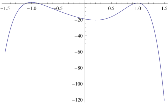
Figure 1: $y=-18.98-13.15x+23.54x^{2}+25.43x^{3}+13.96x^{4}-12.63x^{5}-17.15x^{6}$

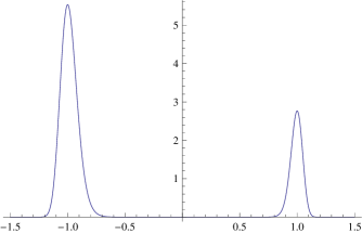
Figure 2: $y=\exp(-18.98-13.15x+23.54x^{2}+25.43x^{3}+13.96x^{4}-12.63x^{5}-17.15x^{6})$

We see that normal mixtures and exponential families have a broadly similar power to describe the qualitative shape of a distribution using only a small number of parameters. Our hope is that by approximating the probability distributions that occur in the Kushner–Stratonovich equation by elements of one of these families we will be able to derive a low dimensional approximation to the full infinite dimensional stochastic partial differential equation.

3.2 Two Hilbert spaces of probability distributions

We have given direct parameterisations of our families of probability distributions and thus we have implicitly represented them as finite dimensional manifolds. In this section we will see how families of probability distributions can be thought of as being embedded in a Hilbert space and hence they inherit a manifold structure and metric from this Hilbert space.

There are two obvious ways of thinking of embedding a probability density function on ${\mathbb{R}}^{n}$ in a Hilbert space. The first is to simply assume that the probability density function is square integrable and hence lies directly in $L^{2}({\mathbb{R}}^{n})$. The second is to use the fact that a probability density function lies in $L^{1}({\mathbb{R}}^{n})$ and is non-negative almost everywhere. Hence $\sqrt{p}$ will lie in $L^{2}({\mathbb{R}}^{n})$.

For clarity we will write $L^{2}_{D}({\mathbb{R}}^{n})$ when we think of $L^{2}({\mathbb{R}}^{n})$ as containing densities directly. The $D$ stands for direct. We write ${\cal D}\subset L^{2}_{D}({\mathbb{R}}^{n})$ where ${\cal D}$ is the set of square integrable probability densities (functions with integral $1$ which are positive almost everywhere).

Similarly we will write $L^{2}_{H}({\mathbb{R}}^{n})$ when we think of $L^{2}({\mathbb{R}}^{n})$ as being a space of square roots of densities. The $H$ stands for Hellinger (for reasons we will explain shortly). We will write ${\cal H}$ for the subset of $L^{2}_{H}$ consisting of square roots of probability densities.

We now have two possible ways of formalizing the notion of a family of probability distributions. In the next section we will define a smooth family of distributions to be either a smooth submanifold of $L^{2}_{D}$ which also lies in ${\cal D}$ or a smooth submanifold of $L^{2}_{H}$ which also lies in ${\cal H}$. Either way the families we discussed earlier will give us finite dimensional families in this more formal sense.

The Hilbert space structures of $L^{2}_{D}$ and $L^{2}_{H}$ allow us to define two notions of distance between probability distributions which we will denote $d_{D}$ and $d_{H}$. Given two probability distributions $p_{1}$ and $p_{2}$ we have an injection $\iota$ into $L^{2}$ so one defines the distance to be the norm of $\iota(p_{1})-\iota(p_{2})$. So given two probability densities $p_{1}$ and $p_{2}$ on ${\mathbb{R}}^{n}$ we can define:

$$d_{H}(p_{1},p_{2}) = \left(\int(\sqrt{p_{1}}-\sqrt{p_{2}})^{2}{\mathrm{d}}\mu\right)^{\frac{1}{2}}$$

$$d_{D}(p_{1},p_{2}) = \left(\int(p_{1}-p_{2})^{2}{\mathrm{d}}\mu\right)^{\frac{1}{2}}.$$

Here ${\mathrm{d}}\mu$ is the Lebesgue measure. $d_{H}$ defines the Hellinger distance between the two distributions, which explains are use of $H$ as a subscript. We will write $\langle\cdot,\cdot\rangle_{H}$ for the inner product associated with $d_{H}$ and $\langle\cdot,\cdot\rangle_{D}$ or simply $\langle\cdot,\cdot\rangle$ for the inner product associated with $d_{D}$.

In this paper we will consider the projection of the conditional density of the true state of the system given the observations (which is assumed to lie in ${\cal D}$ or ${\cal H}$) onto a submanifold. The notion of projection only makes sense with respect to a particular inner product structure. Thus we can consider projection using $d_{H}$ or projection using $d_{D}$. Each has advantages and disadvantages.

The most notable advantage of the Hellinger metric is that the $d_{H}$ metric can be defined independently of the Lebesgue measure and its definition can be extended to define the distance between measures without density functions (see Jacod and Shiryaev [25]). In particular the Hellinger distance is indepdendent of the choice of parameterization for ${\mathbb{R}}^{n}$. This is a very attractive feature in terms of the differential geometry of our set up.

Despite the significant theoretical advantages of the $d_{H}$ metric, the $d_{D}$ metric has an obvious advantage when studying mixture families: it comes from an inner product on $L^{2}_{D}$ and so commutes with addition on $L^{2}_{D}$. So it should be relatively easy to calculate with the $d_{D}$ metric when adding distributions as happens in mixture families. As we shall see in practice, when one performs concrete calculations, the $d_{H}$ metric works well for exponential families and the $d_{D}$ metric works well for mixture families.

3.3 The tangent space of a family of distributions

To make our notion of smooth families precise we need to explain what we mean by a smooth map into an infinite dimensional space.

Let $U$ and $V$ be Hilbert spaces and let $f:U\to V$ be a continuous map ($f$ need only be defined on some open subset of $U$). We say that $f$ is Frećhet differentiable at $x$ if there exists a bounded linear map $A:U\to V$ satisfying:

$$\lim_{h\to x}\frac{\|f(h)-f(x)-Ah\|_{V}}{\|h\|_{U}}$$

If $A$ exists it is unique and we denote it by ${\mathrm{D}}f(x)$. This limit is called the Frećhet derivative of $f$ at $x$. It is the best linear approximation to $f$ at $0$ in the sense of minimizing the norm on $V$.

This allows us to define a smooth map $f:U\to V$ defined on an open subset of $U$ to be an infinitely Frećhet differentiable map. We define an immersion of an open subset of ${\mathbb{R}}^{n}$ into $V$ to be a map such that ${\mathrm{D}}f(x)$ is injective at every point where $f$ is defined. The latter condition ensures that the best linear approximation to $f$ is a genuinely $n$ dimensional map.

Given an immersion $f$ defined on a neighbourhood of $x$, we can think of the vector subspace of $V$ given by the image of ${\mathrm{D}}f(x)$ as representing the tangent space at $x$.

To make these ideas more concrete, let us suppose that $p(\theta)$ is a probability distribution depending smoothly on some parameter $\theta=(\theta_{1},\theta_{2},\ldots,\theta_{m})\in U$ where $U$ is some open subset of ${\mathbb{R}}^{m}$. The map $\theta\to p(\theta)$ defines a map $i:U\to{\cal D}$. At a given point $\theta\in U$ and for a vector $h=(h_{1},h_{2},\ldots,h_{m})\in{\mathbb{R}}^{m}$ we can compute the Fréchet derivative to obtain:

$${\mathrm{D}}i(\theta)h=\sum_{i=1}^{m}\frac{\partial p}{\partial\theta_{i}}h_{i}$$

So we can identify the tangent space at $\theta$ with the following subspace of $L^{2}_{D}$:

$${\rm span}\{\frac{\partial p}{\partial\theta_{1}},\frac{\partial p}{\partial\theta_{2}},\ldots,\frac{\partial p}{\partial\theta_{m}}\}$$ (5)

We can formally define a smooth $n$-dimensional family of probability distributions in $L^{2}_{D}$ to be an immersion of an open subset of ${\mathbb{R}}^{n}$ into ${\cal D}$. Equivalently it is a smoothly parameterized probability distribution $p$ such that the above vectors in $L^{2}$ are linearly independent.

We can define a smooth $m$-dimensional family of probability distributions in $L^{2}_{H}$ in the same way. This time let $q(\theta)$ be a square root of a probability distribution depending smoothly on $\theta$. The tangent vectors in this case will be the partial derivatives of $q$ with respect to $\theta$. Since one normally prefers to work in terms of probability distributions rather than their square roots we use the chain rule to write the tangent space as:

$${\rm span}\{\frac{1}{2\sqrt{p}}\frac{\partial p}{\partial\theta_{1}},\frac{1}{2\sqrt{p}}\frac{\partial p}{\partial\theta_{2}},\ldots,\frac{1}{2\sqrt{p}}\frac{\partial p}{\partial\theta_{m}}\}$$ (6)

We have defined a family of distributions in terms of a single immersion $f$ into a Hilbert space $V$. In other words we have defined a family of distributions in terms of a specific parameterization of the image of $f$. It is tempting to try and phrase the theory in terms of the image of $f$. To this end, one defines an embedded submanifold of $V$ to be a subspace of $V$ which is covered by immersions $f_{i}$ from open subsets of ${\mathbb{R}}^{n}$ where each $f_{i}$ is a homeomorphisms onto its image. With this definition, we can state that the tangent space of an embedded submanifold is independent of the choice of parameterization.

One might be tempted to talk about submanifolds of the space of probability distributions, but one should be careful. The spaces ${\cal H}$ and ${\cal D}$ are not open subsets of $L^{2}_{H}$ and $L^{2}_{D}$ and so do not have any obvious Hilbert-manifold structure. To see why, consider Figure 3 where we have peturbed a probability distribution slightly by subtracting a small delta-like function.

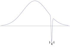
Figure 3: An element of $L^{2}$ arbitrarily close to the normal distribution but not in $H$

3.4 The Fisher information metric

Given two tangent vectors at a point to a family of probability distributions we can form their inner product using $\langle\cdot,\cdot\rangle_{H}$. This defines a so-called Riemannian metric on the family. With respect to a particular parameterization $\theta$ we can compute the inner product of the $i^{th}$ and $j^{th}$ basis vectors given in equation (6). We call this quantity $\frac{1}{4}g_{ij}$.

$$\frac{1}{4}g_{ij}(\theta) := \langle\frac{1}{2\sqrt{p}}\frac{\partial p}{\partial\theta_{i}},\frac{1}{2\sqrt{p}}\frac{\partial p}{\partial\theta_{j}}\rangle_{H}$$

$$= \frac{1}{4}\int\frac{1}{p}\frac{\partial p}{\partial\theta_{i}}\frac{\partial p}{\partial\theta_{j}}{\mathrm{d}}\mu$$

$$= \frac{1}{4}\int\frac{\partial\log p}{\partial\theta_{i}}\frac{\partial\log p}{\partial\theta_{j}}p{\mathrm{d}}\mu$$

$$= \frac{1}{4}E_{p}(\frac{\partial\log p}{\partial\theta_{i}}\frac{\partial\log p}{\partial\theta_{j}})$$

Up to the factor of $\frac{1}{4}$, this last formula is the standard definition for the Fisher information matrix. So our $g_{ij}$ is the Fisher information matrix. We can now interpret this matrix as the Fisher information metric and observe that, up to the constant factor, this is the same thing as the Hellinger distance. See [3], [35] and [1] for more in depth study on this differential geometric approach to statistics.

Example 3.3

The Gaussian family of densities can be parameterized using parameters mean $\mu$ and variance $v$. With this parameterization the Fisher metric is given by:

$$g(\mu,v)=\frac{1}{v}\left[\begin{array}[]{cc}1&0\\ 0&1/(2v)\end{array}\right]$$

The representation of the metric as a matrix depends heavily upon the choice of parameterization for the family.

Example 3.4

The Gaussian family may be considered as a particular exponential family with parameters $\theta_{1}$ and $\theta_{2}$ given by:

$$p(x,\theta)=\exp(\theta_{1}x+\theta_{2}x^{2}-\psi(\theta))$$

where $\psi(\theta)$ is chosen to normalize $p$. It follows that:

$$\psi(\theta)=\frac{1}{2}\log\left(\frac{\pi}{-\theta_{2}}\right)-\frac{{\theta_{1}}^{2}}{4\theta_{2}}$$

This is related to the familiar parameterization in terms of $\mu$ and $v$ by:

$$\mu=-\theta_{1}/(2\theta_{2}),\quad v=\sigma^{2}=(1/\theta_{2}-\theta_{1}^{2}/\theta_{2}^{2})/2$$

One can compute the Fisher information metric relative to the parameterization $\theta_{1}$ to obtain:

$$g(\theta)=\left[\begin{array}[]{cc}-1/(2\theta_{2})&\theta_{1}/(2\theta_{2}^{2})\\ \theta_{1}/(2\theta_{2}^{2})&1/(2\theta_{2}^{2})-\theta_{1}^{2}/(2\theta_{2}^{3})\end{array}\right]$$

The particular importance of the metric structure for this paper is that it allows us to define orthogonal projection of $L^{2}_{H}$ onto the tangent space.

Suppose that one has $m$ linearly independent vectors $w_{i}$ spanning some subspace $W$ of a Hilbert space $V$. By linearity, one can write the orthogonal projection onto $W$ as:

$$\Pi(v)=\sum_{i=1}^{m}[\sum_{i=1}^{m}A^{ij}\langle v,w_{j}\rangle]w_{i}$$

for some appropriately chosen constants $A^{ij}$. Since $\Pi$ acts as the identity on $w_{i}$ we see that $A^{ij}$ must be the inverse of the matrix $A_{ij}=\langle w_{i},w_{j}\rangle$.

We can apply this to the basis given in equation (6). Defining $g^{ij}$ to be the inverse of the matrix $g_{ij}$ we obtain the following formula for projection, using the Hellinger metric, onto the tangent space of a family of distributions:

$$\Pi_{H}(v)=\sum_{i=1}^{m}\left[\sum_{j=1}^{m}4g^{ij}\langle v,\frac{1}{2\sqrt{p}}\frac{\partial p}{\partial\theta_{j}}\rangle_{H}\right]\frac{1}{2\sqrt{p}}\frac{\partial p}{\partial\theta_{i}}$$

3.5 The direct $L^{2}$ metric

The ideas from the previous section can also be applied to the direct $L^{2}$ metric. This gives a different Riemannian metric on the manifold.

We will write $h=h_{ij}$ to denote the $L^{2}$ metric when written with respect to a particular parameterization.

Example 3.5

In coordinates $\mu$, $\nu$, the $L^{2}$ metric on the Gaussian family is:

$$h(\mu,\nu)=\frac{1}{4\nu\sqrt{\nu\pi}}\left[\begin{array}[]{cc}1&0\\ 0&\frac{3}{8\nu}\end{array}\right]$$

We can obtain a formula for projection in $L^{2}_{D}$ using the direct $L^{2}$ metric using the basis given in equation (5). We write $h^{ij}$ for the matrix inverse of $h_{ij}$.

$$\Pi_{D}(v)=\sum_{i=1}^{m}\left[\sum_{j=1}^{m}h^{ij}\left\langle v,\frac{\partial p}{\partial\theta_{j}}\right\rangle_{D}\right]\frac{\partial p}{\partial\theta_{i}}.$$ (7)

4 The projection filter

Given a family of probability distributions parameterised by $\theta$, we wish to approximate an infinte dimensional solution to the non-linear filtering SPDE using elements of this family. Thus we take the Kushner–Stratonovich equation (4), view it as defining a stochastic vector field in ${\cal D}$ and then project that vector field onto the tangent space of our family. The projected equations can then be viewed as giving a stochastic differential equation for $\theta$. In this section we will write down these projected equations explicitly.

Let $\theta\to p(\theta)$ be the parameterization for our family. A curve $t\to\theta(t)$ in the parameter space corresponds to a curve $t\to p(\cdot,\theta(t))$ in ${\cal D}$. For such a curve, the left hand side of the Kushner–Stratonovich equation (4) can be written:

$$d_{t}p(\cdot,\theta(t)) = \sum_{i=1}^{m}\frac{\partial p(\cdot,\theta(t))}{\partial\theta_{i}}d_{t}\theta_{i}(t)$$

$$= \sum_{i=1}^{m}v_{i}{\mathrm{d}}\theta_{i}$$

where we write $v_{i}=\frac{\partial p}{\partial\theta_{i}}$. $\{v_{i}\}$ is the basis for the tangent space of the manifold at $\theta(t)$.

Given the projection formula given in equation (7), we can project the terms on the right hand side onto the tangent space of the manifold using the direct $L^{2}$ metric as follows:

$$\Pi_{D}^{\theta}[{\cal L}^{*}p] = \sum_{i=1}^{m}\left[\sum_{j=1}^{m}h^{ij}\langle{\cal L}^{*}p,v_{j}\rangle\right]v_{i}$$

$$= \sum_{i=1}^{m}\left[\sum_{j=1}^{m}h^{ij}\langle p,{\cal L}v_{j}\rangle\right]v_{i}$$

$$\Pi_{D}^{\theta}[\gamma^{k}(p)] = \sum_{i=1}^{m}\left[\sum_{j=1}^{m}h^{ij}\langle\gamma^{k}(p),v_{j}\rangle\right]v_{i}$$

Thus if we take $L^{2}$ projection of each side of equation (4) we obtain:

$$\sum_{i=1}^{m}v_{i}{\mathrm{d}}\theta^{i}=\sum_{i=1}^{m}\left[\sum_{j=1}^{m}h^{ij}\left\{\langle p,{\cal L}v_{j}\rangle{\mathrm{d}}t-\langle\gamma^{0}(p),v_{j}\rangle{\mathrm{d}}t+\sum_{k=1}^{d}\langle\gamma^{k}(p),v_{j}\rangle\circ{\mathrm{d}}Y^{k}\right\}\right]v_{i}$$

Since the $v_{i}$ form a basis of the tangent space, we can equate the coefficients of $v_{i}$ to obtain:

$${\mathrm{d}}\theta^{i}=\sum_{j=1}^{m}h^{ij}\left\{\langle p(\theta),{\cal L}v_{j}\rangle{\mathrm{d}}t-\langle\gamma^{0}(p(\theta)),v_{j}\rangle{\mathrm{d}}t+\sum_{k=1}^{d}\langle\gamma^{k}(p(\theta)),v_{j}\rangle\circ{\mathrm{d}}Y^{k}\right\}.$$ (8)

This is the promised finite dimensional stochastic differential equation for $\theta$ corresponding to $L^{2}$ projection.

If preferred, one could instead project the Kushner–Stratonovich equation using the Hellinger metric instead. This yields the following stochastic differential equation derived originally in [14]:

$${\mathrm{d}}\theta_{i}=\sum_{j=1}^{m}g^{ij}\left(\langle\frac{{\cal L}^{*}p}{p},v_{j}\rangle{\mathrm{d}}t-\langle\frac{1}{2}|b|^{2},v_{j}\rangle{\mathrm{d}}t+\sum_{k=1}^{d}\langle b^{k},v_{j}\rangle\circ{\mathrm{d}}Y^{k}\right)$$ (9)

Note that the inner products in this equation are the direct $L^{2}$ inner products: we are simply using the $L^{2}$ inner product notation as a compact notation for integrals.

Finally, it is now possible to explain why we resorted to the KS Equation for the optimal filter rather than the Zakai equation in deriving the projection filter.

4.1 Projecting Kushner-Stratonovich vs Zakai

Consider the nonlinear terms in the KS Equation (4), namely

$${\textstyle\frac{1}{2}}\,p_{t}\,E_{p_{t}}\{|b_{t}|^{2}\}\,dt,\ \ \ \sum_{k=1}^{d}p_{t}\,[-E_{p_{t}}\{b_{t}^{k}\}]\circ dY_{t}^{k}.$$

Consider first the Hellinger projection filter (9). By inspection, we see that there is no impact of the nonlinear terms in the projected equation. Therefore, we see that projecting the Zakai unnormalized density SPDE in Hellinger metric onto the statistical manifold $p(\cdot,\theta)$ results in the same projection filter equation as projecting the normalized density KS SPDE. In other words, in Hellinger/Fisher metric the projection automatically takes care of normalization, so we could work with Zakai without changing the result. Intuitively, this happens because, under Hellinger, the set of square roots of normalized densities forms a unit sphere, and the tangent space is orthogonal to the direction corresponding to scaling (Hanzon 1987 [22] uses Zakai rather than KS for this reason, among others). To see this, let us set $q_{t}(x)=\alpha_{t}p(x;\theta_{t})$, so that $\alpha_{t}=\int q_{t}(x)dx$, and calculate ($d_{t}$ is short-hand for a Stratonovich differential)

$$\langle d_{t}\sqrt{q_{t}(x)},\frac{\partial\sqrt{p(x;\theta_{t})}}{\partial\theta_{i}}\rangle=\frac{1}{4\sqrt{\alpha}}\langle(d\alpha_{t}),\frac{\partial{p(x;\theta_{t})}}{\partial\theta_{i}}\rangle+\sqrt{\alpha}\sum_{k}g_{k,i}(\theta)\circ d\theta_{k}\$$

and

$$\langle(d\alpha_{t}),\frac{\partial{p(x;\theta_{t})}}{\partial\theta_{i}}\rangle=(d\alpha)\frac{\partial}{\partial\theta_{i}}\int p(x;\theta)dx=(d\alpha)\ \frac{\partial 1}{\partial\theta_{i}}=0$$

so that the component corresponding to change in the scaling constant does not contribute to the projection.

The main focus of this paper, however, is the $d_{D}$ projection filter (8). For this filter we do have an impact of the nonlinear terms. In fact, it is easy to adapt the derivation of the $d_{D}$ filter to the Zakai equation, which leads to the following new filter, namely the $d_{D}$ Zakai projection filter:

$${\mathrm{d}}\theta^{i}=\sum_{j=1}^{m}h^{ij}\left\{\langle p(\theta),{\cal L}v_{j}\rangle{\mathrm{d}}t-\langle{\textstyle\frac{1}{2}}\,|b_{t}|^{2}\ p(\theta),v_{j}\rangle{\mathrm{d}}t+\sum_{k=1}^{d}\langle b_{t}^{k}\ p(\theta),v_{j}\rangle\circ{\mathrm{d}}Y^{k}\right\}.$$ (10)

This filter is clearly different from (8). We have implemented (10) for the sensor case, using a simple variation on the numerical algorithms below. We found that (10) gives slightly worse results for the $L^{2}$ residual of the normalized density than (8). This can be explained simply by the fact that if we want to approximate $p$ in a given norm then we should project an equation for $p$ whereas if we wish to approximate $q$ we should project an equation for $q$. The fact that $\sqrt{q}$ has variable $L^{2}$ norm in time is not relevant for the projection in the Hellinger metric, while it is for the $d_{D}$ metric, where the lack of normalization in the Zakai Eq. density plays a role in the projection.

5 Equivalence with ADFs and Galerkin Methods

The projection filter with specific metrics and manifolds can be shown to be equivalent to earlier filtering algorithms. In particular, while the $d_{H}$ metric leads to the Fisher Information and to an equivalence between the projection filter and Assumed Density Filters (ADFs) when using exponential families, see [13], the $d_{D}$ metric for simple mixture families is equivalent to a Galerkin method, as we show now following the second named author preprint [11].

For applications of Galerkin methods to Nonlinear filtering we refer for example to [36], [21], [24], [6].

The basic Galerkin approximation is obtained by approximating the exact solution of the filtering SPDE (4) with a linear combination of basis functions $\phi_{i}(x)$, namely

$$\tilde{p}_{t}(x):=\sum_{i=1}^{\ell}c_{i}(t)\phi_{i}(x).$$ (11)

Ideally, the $\phi_{i}$ can be extended to indices $\ell+1,\ell+2,\ldots,+\infty$ so as form a basis of $L^{2}$.

The method can be sketched intuitively as follows. We could write the filtering equation (4) as

$$\langle-d{p}_{t}+{\cal L}_{t}^{\ast}\,{p}_{t}\,dt-\gamma_{t}^{0}({p}_{t})\,dt+\sum_{k=1}^{d}\gamma_{t}^{k}({p}_{t})\circ dY_{t}^{k}\ ,\xi\rangle=0$$

for all smooth $L^{2}$ test functions $\xi$ such that the inner product exists.

We replace this equation with the equation

$$\langle-d\tilde{p}_{t}+{\cal L}_{t}^{\ast}\,\tilde{p}_{t}\,dt-\gamma_{t}^{0}(\tilde{p}_{t})\,dt+\sum_{k=1}^{d}\gamma_{t}^{k}(\tilde{p}_{t})\circ dY_{t}^{k}\ ,\phi_{j}\rangle=0,\ \ j=1,\ldots,\ell.$$

By substituting Equation (11) in this last equation, using the linearity of the inner product in each argument and by using integration by parts we obtain easily an equation for the combinators $c$, namely

$$\sum_{i=1}^{\ell}\langle\phi_{i},\phi_{j}\rangle dc_{i}=\sum_{i=1}^{\ell}\langle\phi_{i},{\cal L}\phi_{j}\rangle c_{i}\ dt-\langle\gamma_{t}^{0}\left(\sum_{h=1}^{\ell}c_{h}\phi_{h}\right),\phi_{j}\rangle$$ (12)

$$+\sum_{k=1}^{d}\langle\gamma_{t}^{k}\left(\sum_{h=1}^{\ell}c_{h}\phi_{h}\right),\phi_{j}\rangle\circ dY_{t}^{k}$$

Consider now the projection filter with the following choice of the manifold. We use the convex hull of a set of basic $L^{2}$ probability densities $q_{1},\ldots,q_{m+1}$, namely the basic mixture family

$$\{p(\theta):=\theta_{1}q_{1}+\ldots+\theta_{m}q_{m}+[1-(\theta_{1}+\ldots+\theta_{m})]q_{m+1},\ \sum_{i=1}^{m}\theta_{i}<1,\ \theta_{i}\geq 0\ \mbox{for all}\ \ i\}.$$ (13)

We can see easily that tangent vectors for the $d_{2}$ structure and the matrix $h$ are

$$v_{j}=q_{j}-q_{m+1},\ \ \ h_{i,j}=\langle q_{i}-q_{m+1},q_{j}-q_{m+1}\rangle,\ \ i,j=1,\ldots,m.$$

so that the metric is constant in $\theta$. If we apply the $d_{2}$ projection filter Equation (8) with this choice of manifold, we see immediately by inspection that this equation coincides with the Galerkin method Equation (12) if we take

$$\ell=m+1,\ c_{i}=\theta_{i}\ \mbox{and}\ \phi_{i}=q_{i}-q_{m+1}\ \mbox{for}\ i=1,\ldots,m,\ \mbox{and}\ c_{m+1}=1,\ \phi_{m+1}=q_{m+1}.$$

The choice of the simple mixture is related to a choice of the $L^{2}$ basis in the Galerkin method. A typical choice could be based on Gaussian radial basis functions, see for example [31].

We have thus proven the following first main theoretical result of this paper:

Theorem 5.1

For simple mixture families (13), the $d_{2}$ projection filter (8) coincides with a Galerkin method (12) where the basis functions are the mixture components $q$.

However, this equivalence holds only for the case where the manifold on which we project is the simple mixture family (13). More complex families, such as the ones we will use in the following, will not allow for a Galerkin-based filter and only the $L^{2}$ projection filter can be defined there. Note also that even in the simple case (13) our $L^{2}$ Galerkin/projection filter will be different from the Galerkin projection filter seen for example in [6], because we use Stratonovich calculus to project the Kushner-Stratonovich equation in $L^{2}$ metric. In [6] the Ito version of the Kushner-Stratonovich Equation is used instead for the Galerkin method, but since Ito calculus does not work on manifolds, due to the second order term moving the dynamics out of the tangent space (see for example [10]), we use the Stratonovich version instead. The Ito-based and Stratonovich based Galerkin projection filters will therefore differ for simple mixture families, and again, only the second one can be defined for manifolds of densities beyond the simplest mixture family.

6 Numerical Software Design

Equations (8) and (9) both give finite dimensional stochastic differential equations that we hope will approximate well the solution to the full Kushner–Stratonovich equation. We wish to solve these finite dimensional equations numerically and thereby obtain a numerical approximation to the non-linear filtering problem.

Because we are solving a low dimensional system of equations we hope to end up with a more efficient scheme than a brute-force finite difference approach. A finite difference approach can also be seen as a reduction of the problem to a finite dimensional system. However, in a finite difference approach the finite dimensional system still has a very large dimension, determined by the number of grid points into which one divides ${\mathbb{R}}^{n}$. By contrast the finite dimensional manifolds we shall consider will be defined by only a handful of parameters.

The specific solution algorithm will depend upon numerous choices: whether to use $L^{2}$ or Hellinger projection; which family of probability distributions to choose; how to parameterize that family; the representation of the functions $f$, $\sigma$ and $b$; how to perform the integrations which arise from the calculation of expectations and inner products; the numerical method selected to solve the finite dimensional equations.

To test the effectiveness of the projection idea, we have implemented a C++ engine which performs the numerical solution of the finite dimensional equations and allows one to make various selections from the options above. Currently our implementation is restricted to the case of the direct $L^{2}$ projection for a $1$-dimensional state $X$ and $1$-dimensional noise $W$. However, the engine does allow one to experiment with various manifolds, parameteriziations and functions $f$, $\sigma$ and $b$.

We use object oriented programming techniques in order to allow this flexibility. Our implementation contains two key classes FunctionRing and Manifold.

To perform the computation, one must choose a data structure to represent elements of the function space. However, the most effective choice of representation depends upon the family of probability distributions one is considering and the functions $f$, $\sigma$ and $b$. Thus the C++ engine does not manipulate the data structure directly but instead works with the functions via the FunctionRing interface. A UML (Unified Modelling Language [39]) outline of the FunctionRing interface is given in table 1.

FunctionRing
+ add( $f_{1}$ : Function, $f_{2}$ : Function ) : Function
+ multiply( $f_{1}$ : Function, $f_{2}$ : Function ) : Function
+ multiply( $s$ : Real, $f$ : Function ) : Function
+ differentiate( $f$ : Function ) : Function
+ integrate( $f$ : Function ) : Real
+ evaluate( $f$ : Function ) : Real
+ constantFunction( $s$ : Real ) : Function

Table 1: UML for the FunctionRing interface

Manifold
+ getRing() : FunctionRing
+ getDensity( $\theta$ ) : Function
+ computeTangentVectors( $\theta$ : Point ) : Function*
+ updatePoint( $\theta$ : Point, $\Delta\theta$ : Real* ) : Point
+ finalizePoint( $\theta$ : Point ) : Point

Table 2: UML for the Manifold interface

The other key abstraction is the Manifold. We give a UML representation of this abstraction in table 2. For readers unfamiliar with UML, we remark that the $*$ symbol can be read “list”. For example, the computeTangentVectors function returns a list of functions.

The Manifold uses some convenient internal representation for a point, the most obvious representation being simply the $m$-tuple $(\theta_{1},\theta_{2},\ldots\theta_{m})$. On request the Manifold is able to provide the density associated with any point represented as an element of the FunctionRing.

In addition the Manifold can compute the tangent vectors at any point. The computeTangentVectors method returns a list of elements of the FunctionRing corresponding to each of the vectors $v_{i}=\frac{\partial p}{\partial\theta_{i}}$ in turn. If the point is represented as a tuple $\theta=(\theta_{1},\theta_{2},\ldots\theta_{n})$, the method updatePoint simply adds the components of the tuple $\Delta\theta$ to each of the components of $\theta$. If a different internal representation is used for the point, the method should make the equivalent change to this internal representation.

The finalizePoint method is called by our algorithm at the end of every time step. At this point the Manifold implementation can choose to change its parameterization for the state. Thus the finalizePoint allows us (in principle at least) to use a more sophisticated atlas for the manifold than just a single chart.

One should not draw too close a parallel between these computing abstractions and similarly named mathematical abstractions. For example, the space of objects that can be represented by a given FunctionRing do not need to form a differential ring despite the differentiate method. This is because the differentiate function will not be called infinitely often by the algorithm below, so the functions in the ring do not need to be infinitely differentiable.

Similarly the finalizePoint method allows the Manifold implementation more flexibility than simply changing chart. From one time step to the next it could decide to use a completely different family of distributions. The interface even allows the dimension to change from one time step to the next. We do not currently take advantage of this possibility, but adapatively choosing the family of distributions would be an interesting topic for further research.

6.1 Outline of the algorithm

The C++ engine is initialized with a Manifold object, a copy of the initial Point and Function objects representing $f$, $\sigma$ and $b$.

At each time point the engine asks the manifold to compute the tangent vectors given the current point. Using the multiply and integrate functions of the class FunctionRing, the engine can compute the inner products of any two functions, hence it can compute the metric matrix $h_{ij}$. Similarly, the engine can ask the manifold for the density function given the current point and can then compute ${\cal L}^{*}p$. Proceeding in this way, all the coefficients of ${\mathrm{d}}t$ and $\circ{\mathrm{d}}Y$ in equation (8) can be computed at any given point in time.

Were equation (8) an Itô SDE one could now numerically estimate $\Delta\theta$, the change in $\theta$ over a given time interval $\Delta$ in terms of $\Delta$ and $\Delta Y$, the change in $Y$. One would then use the updateState method to compute the new point and then one could repeat the calculation for the next time interval. In other words, were equation (8) an Itô SDE we could numerically solve the SDE using the Euler scheme.

However, equation (8) is a Stratonovich SDE so the Euler scheme is no longer valid. Various numerical schemes for solving stochastic differential equations are considered in [15] and [30]. One of the simplest is the Stratonovich–Heun method described in [15]. Suppose that one wishes to solve the SDE:

$${\mathrm{d}}y_{t}=f(y_{t}){\mathrm{d}}t+g(y_{t})\circ{\mathrm{d}}W_{t}$$

The Stratonvich–Heun method generates an estimate for the solution $y_{n}$ at the $n$-th time interval using the formulae:

$$Y_{n+1} = y_{n}+f(y_{n})\Delta+g(y_{n})\Delta W_{n}$$

$$y_{n+1} = y_{n}+\frac{1}{2}(f(y_{n})+f(Y_{n+1}))\Delta+\frac{1}{2}(g(y_{n})+g(Y_{n+1}))\Delta W_{n}$$

In these formulae $\Delta$ is the size of the time interval and $\Delta W_{n}$ is the change in $W$. One can think of $Y_{n+1}$ as being a prediction and the value $y_{n+1}$ as being a correction. Thus this scheme is a direct translation of the standard Euler–Heun scheme for ordinary differential equations.

We can use the Stratonovich–Heun method to numerically solve equation  (8). Given the current value $\theta_{n}$ for the state, compute an estimate for $\Delta\theta_{n}$ by replacing ${\mathrm{d}}t$ with $\Delta$ and ${\mathrm{d}}W$ with $\Delta W$ in equation (8). Using the updateState method compute a prediction $\Theta_{n+1}$. Now compute a second estimate for $\Delta\theta_{n}$ using equation (8) in the state $\Theta_{n+1}$. Pass the average of the two estimates to the updateState function to obtain the the new state $\theta_{n+1}$.

At the end of each time step, the method finalizeState is called. This provides the manifold implementation the opportunity to perform checks such as validation of the state, to correct the normalization and, if desired, to change the representation it uses for the state.

One small observation worth making is that the equation (8) contains the term $h^{ij}$, the inverse of the matrix $h_{ij}$. However, it is not necessary to actually calculate the matrix inverse in full. It is better numerically to multiply both sides of equation (8) by the matrix $h_{ij}$ and then compute ${\mathrm{d}}\theta$ by solving the resulting linear equations directly. This is the approach taken by our algorithm.

As we have already observed, there is a wealth of choices one could make for the numerical scheme used to solve equation (8), we have simply selected the most convenient. The existing Manifold and FunctionRing implementations could be used directly by many of these schemes — in particular those based on Runge–Kutta schemes. In principle one might also consider schemes that require explicit formulae for higher derivatives such as $\frac{\partial^{2}p}{\partial\theta_{i}\partial\theta_{j}}$. In this case one would need to extend the manifold abstraction to provide this information.

Similarly one could use the same concepts in order to solve equation (9) where one uses the Hellinger projection. In this case the FunctionRing would need to be extended to allow division. This would in turn complicate the implementation of the integrate function, which is why we have not yet implemented this approach.

7 The case of normal mixture families

We now apply the above framework to normal mixture families. Let ${\cal R}$ denote the space of functions which can be written as finite linear combinations of terms of the form:

$$\pm x^{n}e^{ax^{2}+bx+c}$$

where $n$ is non-negative integer and $a$, $b$ and $c$ are constants. ${\cal R}$ is closed under addition, multiplication and differentiation, so it forms a differential ring.

We have written an implementation of FunctionRing corresponding to ${\cal R}$. Although the implementation is mostly straightforward some points are worth noting.

Firstly, we store elements of our ring in memory as a collection of tuples $(\pm,a,b,c,n)$. Although one can write:

$$\pm x^{n}e^{ax^{2}+bx+c}=qx^{n}e^{ax^{2}+bx}$$

for appropriate $q$, the use or such a term in computer memory should be avoided as it will rapidly lead to significant rounding errors. A small amount of care is required throughout the implementation to avoid such rounding errors.

Secondly let us consider explicitly how to implement integration for this ring. Let us define $u_{n}$ to be the integral of $x^{n}e^{-x^{2}}$. Using integration by parts one has:

$$u_{n}:=\int_{-\infty}^{\infty}x^{n}e^{-x^{2}}{\mathrm{d}}x=\frac{n-1}{2}\int_{-\infty}^{\infty}x^{n-2}e^{-x^{2}}{\mathrm{d}}x=\frac{n-1}{2}u_{n-2}$$

Since $u_{0}=\sqrt{\pi}$ and $u_{1}=0$ we can compute $u_{n}$ recursively. Hence we can analytically compute the integral of $p(x)e^{-x^{2}}$ for any polynomial $p$. By substitution, we can now integrate $p(x-\mu)e^{-(x-\mu)^{2}}$ for any $\mu$. By completing the square we can analytically compute the integral of $p(x)e^{ax^{2}+bx+c}$ so long as $a<0$. Putting all this together one has an algorithm for analytically integrating the elements of ${\cal R}$.

Let ${\cal N}^{i}$ denote the space of probability distributions that can be written as $\sum_{k=1}^{i}c_{k}e^{a_{k}x^{2}+b_{k}x}$ for some real numbers $a_{k}$, $b_{k}$ and $c_{k}$ with $a_{k}<0$. Given a smooth curve $\gamma(t)$ in ${\cal N}^{i}$ we can write:

$$\gamma(t)=\sum_{k=1}^{i}c_{k}(t)e^{a_{k}(t)x^{2}+b_{k}(t)x}.$$

We can then compute:

$$\frac{{\mathrm{d}}\gamma}{{\mathrm{d}}t} = \sum_{k=1}^{i}\left(\left(\frac{{\mathrm{d}}a_{k}}{{\mathrm{d}}t}x^{2}+\frac{{\mathrm{d}}b_{k}}{{\mathrm{d}}t}x\right)c_{k}e^{a_{k}x^{2}+b_{k}x}+\frac{{\mathrm{d}}c_{k}}{{\mathrm{d}}t}e^{a_{k}x^{2}+b_{k}x}\right)$$

$$\in {\cal R}$$

We deduce that the tangent vectors of any smooth submanifold of ${\cal N}^{i}$ must also lie in ${\cal R}$. In particular this means that our implementation of FunctionRing will be sufficient to represent the tangent vectors of any manifold consisting of finite normal mixtures.

Combining these ideas we obtain the second main theoretical result of the paper.

Theorem 7.1

Let $\theta$ be a parameterization for a family of probability distributions all of which can be written as a mixture of at most $i$ Gaussians. Let $f$, $a=\sigma^{2}$ and $b$ be functions in the ring ${\cal R}$. In this case one can carry out the direct $L^{2}$ projection algorithm for the problem given by equation (1) using analytic formulae for all the required integrations.

Although the condition that $f$, $a$ and $b$ lie in ${\cal R}$ may seem somewhat restrictive, when this condition is not met one could use Taylor expansions to find approximate solutions, although in such case rigorous convergence results need to be established.

Although the choice of parameterization does not affect the choice of FunctionRing, it does affect the numerical behaviour of the algorithm. In particular if one chooses a parameterization with domain a proper subset of ${\mathbb{R}}^{m}$, the algorithm will break down the moment the point $\theta$ leaves the domain. With this in mind, in the numerical examples given later in this paper we parameterize normal mixtures of $k$ Gaussians with a parameterization defined on the whole of ${\mathbb{R}}^{n}$. We describe this parameterization below.

Label the parameters $\xi_{i}$ (with $1\leq i\leq k-1$), $x_{1}$, $y_{i}$ (with $2\leq i\leq k$) and $s_{i}$ (with $1\leq i\leq k$). This gives a total of $3k-1$ parameters. So we can write

$$\theta=(\xi_{1},\ldots,\xi_{k-1},x_{1},y_{2},\ldots,y_{k},s_{1},\ldots,s_{k})$$

Given a point $\theta$ define variables as follows:

$$\lambda_{1} = \operatorname{logit}^{-1}(\xi_{1})$$

$$\lambda_{i} = \operatorname{logit}^{-1}(\xi_{i})(1-\lambda_{1}-\lambda_{2}-\ldots-\lambda_{i-1})\qquad(2\leq i\leq k-1)$$

$$\lambda_{k} = 1-\lambda_{1}-\lambda_{2}-\ldots-\lambda_{k-1}$$

$$x_{i} = x_{i-1}+e^{y_{i}}\qquad(2\leq i\leq k)$$

$$\sigma_{i} = e^{s_{i}}$$

where the $\operatorname{logit}$ function sends a probability $p\in[0,1]$ to its log odds, $\ln(p/1-p)$. We can now write the density associated with $\theta$ as:

$$p(x)=\sum_{i=1}^{k}\lambda_{i}\frac{1}{\sigma_{i}\sqrt{2\pi}}\exp(-\frac{(x-x_{i})^{2}}{2\sigma_{i}^{2}})$$

We do not claim this is the best possible choice of parameterization, but it certainly performs better than some more naïve parameteriations with bounded domains of definition. We will call the direct $L^{2}$ projection algorithm onto the normal mixture family given with this projection the L2NM projection filter.

7.1 Comparison with the Hellinger exponential (HE) projection algorithm

A similar algorithm is described in [12, 13] for projection using the Hellinger metric onto an exponential family. We refer to this as the HE projection filter.

It is worth highlighting the key differences between our algorithm and the exponential projection algorithm described in [12].

• In [12] only the special case of the cubic sensor was considered. It was clear that one could in principle adapt the algorithm to cope with other problems, but there remained symbolic manipulation that would have to be performed by hand. Our algorithm automates this process by using the FunctionRing abstraction.

• When one projects onto an exponential family, the stochastic term in equation (9) simplifies to a term with constant coefficients. This means it can be viewed equally well as either an Itô or Stratonovich SDE. The practical consequence of this is that the HE algorithm can use the Euler–Maruyama scheme rather than the Stratonvoich–Heun scheme to solve the resulting stochastic ODE’s. Moreover in this case the Euler-Maruyama scheme coincides with the generally more precise Milstein scheme.

• In the case of the cubic sensor, the HE algorithm requires one to numerically evaluate integrals such as:

  $$\int_{-\infty}^{\infty}x^{n}\exp(\theta_{1}+\theta_{2}x+\theta_{3}x^{2}+\theta_{4}x^{4}){\mathrm{d}}x$$

  where the $\theta_{i}$ are real numbers. Performing such integrals numerically considerably slows the algorithm. In effect one ends up using a rather fine discretization scheme to evaluate the integral and this somewhat offsets the hoped for advantage over a finite difference method.

8 Numerical Results

In this section we compare the results of using the direct $L^{2}$ projection filter onto a mixture of normal distributions with other numerical methods. In particular we compare it with:

1. A finite difference method using a fine grid which we term the exact filter. Various convergence results are known ([32] and [33]) for this method. In the simulations shown below we use a grid with $1000$ points on the $x$-axis and $5000$ time points. In our simulations we could not visually distinguish the resulting graphs when the grid was refined further justifying us in considering this to be extremely close to the exact result. The precise algorithm used is as described in the section on “Partial Differential Equations Methods” in chapter 8 of Bain and Crisan [8].

2. The extended Kalman filter (EK). This is a somewhat heuristic approach to solving the non-linear filtering problem but which works well so long as one assumes the system is almost linear. It is implemented essentially by linearising all the functions in the problem and then using the exact Kalman filter to solve this linear problem - the details are given in [8]. The EK filter is widely used in applications and so provides a standard benchmark. However, it is well known that it can give wildly innaccurate results for non-linear problems so it should be unsurprising to see that it performs badly for most of the examples we consider.

3. The HE projection filter. In fact we have implemented a generalization of the algorithm given in [14] that can cope with filtering problems where $b$ is an aribtrary polynomial, $\sigma$ is constant and $f=0$. Thus we have been able to examine the performance of the exponential projection filter over a slightly wider range of problems than have previously been considered.

To compare these methods, we have simulated solutions of the equations  (1) for various choices of $f$, $\sigma$ and $b$. We have also selected a prior probability distribution $p_{0}$ for $X$ and then compared the numerical estimates for the probability distribution $p$ at subsequent times given by the different algorithms. In the examples below we have selected a fixed value for the intial state $X_{0}$ rather than drawing at random from the prior distribution. This should have no more impact upon the results than does the choice of seed for the random number generator.

Since each of the approximate methods can only represent certain distributions accurately, we have had to use different prior distributions for each algorithm. To compare the two projection filters we have started with a polynomial exponential distribution for the prior and then found a nearby mixture of normal distributions. This nearby distribution was found using a gradient search algorithm to minimize the numerically estimated $L^{2}$ norm of the difference of the normal and polynomial exponential distributions. As indicated earlier, polynomial exponential distributions and normal mixtures are qualitatively similar so the prior distributions we use are close for each algorithm.

For the extended Kalman filter, one has to approximate the prior distribution with a single Gaussian. We have done this by moment matching. Inevitably this does not always produce satisfactory results.

For the exact filter, we have used the same prior as for the $L^{2}$ projection filter.

8.1 The linear filter

The first test case we have examined is the linear filtering problem. In this case the probability density will be a Gaussian at all times — hence if we project onto the two dimensional family consisting of all Gaussian distributions there should be no loss of information. Thus both projection filters should give exact answers for linear problems. This is indeed the case, and gives some confidence in the correctness of the computer implementations of the various algorithms.

8.2 The quadratic sensor

The second test case we have examined is the quadratic sensor. This is problem (1) with $f=0$, $\sigma=c_{1}$ and $b(x)=c_{2}x^{2}$ for some positive constants $c_{1}$ and $c_{2}$. In this problem the non-injectivity of $b$ tends to cause the distribution at any time to be bimodal. To see why, observe that the sensor provides no information about the sign of $x$, once the state of the system has passed through $0$ we expect the probability density to become approximately symmetrical about the origin. Since we expect the probability density to be bimodal for the quadratic sensor it makes sense to approximate the distribution with a linear combination of two Gaussian distributions.

In Figure 4 we show the probability density as computed by three of the algorithms at 10 different time points for a typical quadratic sensor problem. To reduce clutter we have not plotted the results for the exponential filter. The prior exponential distribution used for this simulation was $p(x)=\exp(0.25-x^{2}+x^{3}-0.25x^{4})$. The initial state was $X_{0}=0$ and $Y_{0}=0$.

As one can see the probability densities computed using the exact filter and the L2NM filter become visually indistinguishable when the state moves away from the origin. The extended Kalman filter is, as one would expect, completely unable to cope with these bimodal distributions. In this case the extended Kalman filter is simply representing the larger of the two modes.

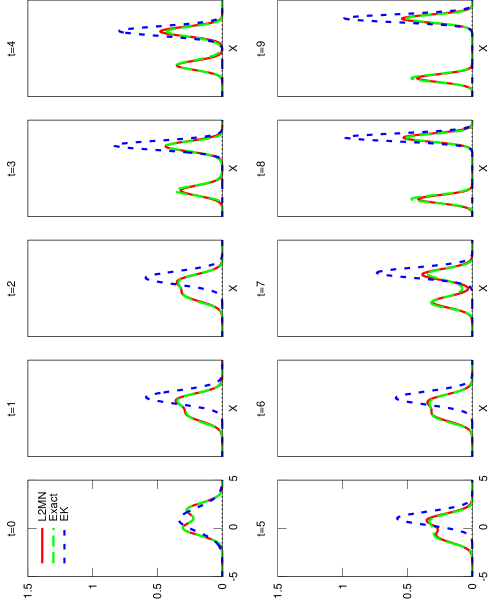
Figure 4: Estimated probability densities at $10$ time points for the problem $b(x)=x^{2}$

In Figure 5 we have plotted the $L^{2}$ residuals for the different algorithms when applied to the quadratic sensor problem. We define the $L^{2}$ residual to be the $L^{2}$ norm of the difference between the exact filter distribution and the estimated distribution.

$$\hbox{$L^{2}$ residual}=\left(\int|p_{\hbox{exact}}-p_{\hbox{approx}}|^{2}{\mathrm{d}}\mu\right)^{\frac{1}{2}}$$

As can be seen, the L2NM projection filter outperforms the HE projection filter when applied to the quadratic sensor problem. Notice that the $L^{2}$ residuals are initially small for both the HE and the L2NM filter. The superior performance of the L2NM projection filter in this case stems from the fact that one can more accurately represent the distributions that occur using the normal mixture family than using the polynomial exponential family.

If preferred one could define a similar notion of residual using the Hellinger metric. The results would be qualitatively similar.

One interesting feature of Figure 5 is that the error remains bounded in size when one might expect the error to accumulate over time. This suggests that the arrival of new measurements is gradually correcting for the errors introduced by the approximation.

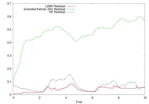
Figure 5: $L^{2}$ residuals for the problem $b(x)=x^{2}$

8.3 The cubic sensor

A third test case we have considered is the general cubic sensor. In this problem one has $f=0$, $\sigma=c_{1}$ for some constant $c_{1}$ and $b$ is some cubic function.

The case when $b$ is a multiple of $x^{3}$ is called the cubic sensor and was used as the test case for the exponential projection filter using the Hellinger metric considered in [14]. It is of interest because it is the simplest case where $b$ is injective but where it is known that the problem cannot be reduced to a finite dimensional stochastic differential equation [23]. It is known from earlier work that the exponential filter gives excellent numerical results for the cubic sensor.

Our new implementations allow us to examine the general cubic sensor. In Figure 6, we have plotted example probability densities over time for the problem with $f=0$, $\sigma=1$ and $b=x^{3}-x$. With two turning points for $b$ this problem is very far from linear. As can be seen in Figure 6 the L2NM projection remains close to the exact distribution throughout. A mixture of only two Gaussians is enough to approximate quite a variety of differently shaped distributions with perhaps surprising accuracy. As expected, the extended Kalman filter gives poor results until the state moves to a region where $b$ is injective. The results of the exponential filter have not been plotted in Figure 6 to reduce clutter. It gave similar results to the L2NM filter.

The prior polynomial exponential distribution used for this simulation was $p(x)=\exp(0.5x^{2}-0.25x^{4})$. The initial state was $X_{0}=0$, which is one of the modes of prior distribution. The inital value for $Y_{0}$ was taken to be $0$.

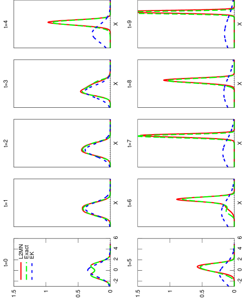
Figure 6: Estimated probability densities at $10$ time points for the problem $b(x)=x^{3}-x$

One new phenomenon that occurs when considering the cubic sensor is that the algorithm sometimes abruptly fails. This is true for both the L2NM projection filter and the HE projection filter.

To show the behaviour over time more clearly, in Figure 7 we have shown a plot of the mean and standard deviation as estimated by the L2NM projection filter against the actual mean and standard deviation. We have also indicated the true state of the system. The mean for the L2MN filter drops to $0$ at approximately time $7$. It is at this point that the algorithm has failed.

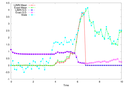
Figure 7: Estimates for the mean and standard deviation for the problem $b(x)=x^{3}-x$

What has happened is that as the state has moved to a region where the sensor is reasonably close to being linear, the probability distribution has tended to a single normal distribution. Such a distribution lies on the boundary of the family consisting of a mixture of two normal distributions. As we approach the boundary, $h_{ij}$ ceases to be invertible causing the failure of the algorithm. Analogous phenomena occur for the exponential filter.

The result of running numerous simulations suggests that the HE filter is rather less robust than the L2NM projection filter. The typical behaviour is that the exponential filter maintains a very low residual right up until the point of failure. The L2NM projection filter on the other hand tends to give slightly inaccurate results shortly before failure and can often correct itself without failing.

This behaviour can be seen in Figure 8. In this figure, the residual for the exponential projection remains extremely low until the algorithm fails abruptly - this is indicated by the vertical dashed line. The L2NM filter on the other hand deteriorates from time $6$ but only fails at time $7$.

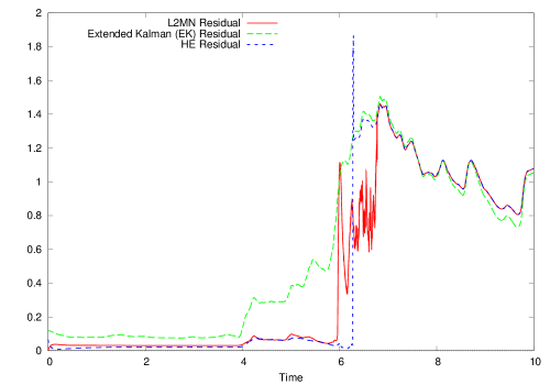
Figure 8: $L^{2}$ residuals for the problem $b(x)=x^{3}-x$

The $L^{2}$ residuals of the L2MN method are rather large between times $6$ and $7$ but note that the accuracy of the estimates for the mean and standard deviation in Figure 7 remain reasonable throughout this time. To understand this note that for two normal distributions with means a distance $x$ apart, the $L^{2}$ distance between the distributions increases as the standard deviations of the distributions drop. Thus the increase in $L^{2}$ residuals between times $6$ and $7$ is to a large extent due to the drop in standard deviation between these times. As a result, one may feel that the $L^{2}$ residual doesn’t capture precisely what it means for an approximation to be “good”. In the next section we will show how to measure residuals in a way that corresponds more closely to the intuitive idea of them having visually similar distribution functions. In practice one’s definition of a good approximation will depend upon the application.

Although one might argue that the filter is in fact behaving reasonably well between times $6$ and $7$ it does ultimately fail. There is an obvious fix for failures like this. When the current point is sufficiently close to the boundary of the manifold, simply approximate the distribution with an element of the boundary. In other words, approximate the distribution using a mixture of fewer Gaussians. Since this means moving to a lower dimensional family of distributions, the numerical implementation will be more efficient on the boundary. This will provide a temporary fix the failure of the algorithm, but it raises another problem: as the state moves back into a region where the problem is highly non linear, how can one decide how to leave the boundary and start adding additional Gaussians back into the mixture? We hope to address this question in a future paper.

9 Comparison with Particle Methods

Particle methods approximate the probability density $p$ using discrete measures of the form:

$$\sum_{i}a_{i}(t)\delta_{v_{i}(t)}$$

These measures are generated using a Monte Carlo method. The measure can be thought of as the empirical distributions associated with randomly located particles at position $v_{i}(t)$ and of stochastic mass $a_{i}(t)$.

Particle methods are currently some of the most effective numerical methods for solving the filtering problem. See [8] and the references therein for details of specific particle methods and convergence results.

The first issue in comparing projection methods with particle methods is that, as a linear combination of Dirac masses, one can only expect a particle method to converge weakly to the exact solution. In particular the $L^{2}$ metric and the Hellinger metric are both inappropriate measures of the residual between the exact solution and a particle approximation. Indeed the $L^{2}$ distance is not defined and the Hellinger distance will always take the value $\sqrt{2}$.

To combat this issue, we will measure residuals using the Lévy metric. If $p$ and $q$ are two probability measures on ${\mathbb{R}}$ and $P$ and $Q$ are the associated cumulative distribution functions then the Lévy metric is defined by:

$$d_{L}(p,q)=\inf\{\epsilon:P(x-\epsilon)-\epsilon\leq Q(x)\leq P(x+\epsilon)+\epsilon\quad\forall x\}$$

This can be interpreted geometrically as the size of the largest square with sides parallel to the coordinate axes that can be inserted between the completed graphs of the cumulative distribution functions (the completed graph of the distribution function is simply the graph of the distribution function with vertical line segments added at discontinuities).

The Lévy metric can be seen as a special case of the Lévy–Prokhorov metric. This can be used to measure the distance between measures on a general metric space. For Polish spaces, the Lévy–Prokhorov metric metrises the weak convergence of probability measures [7]. Thus the Lévy metric provides a reasonable measure of the residual of a particle approximation. We will call residuals measured in this way Lévy residuals.

A second issue in comparing projection methods with particle methods is deciding how many particles to use for the comparison. A natural choice is to compare a projection method onto an $m$-dimensional manifold with a particle method that approximates the distribution using $\lceil(m+1)/2\rceil$ particles. In other words, equate the dimension of the families of distributions used for the approximation.

A third issue is deciding which particle method to choose for the comparison from the many algorithms that can be found in the literature. We can work around this issue by calculating the best possible approximation to the exact distribution that can be made using $\lceil(m+1)/2\rceil$ Dirac masses. This approach will substantially underestimate the Lévy residual of a particle method: being Monte Carlo methods, large numbers of particles would be required in practice.

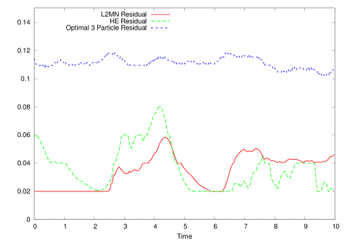
Figure 9: Lévy residuals for the problem $b(x)=x^{2}$

In Figure 9 we have plotted bounds on the Lévy residuals for the two projection methods for the quadratic sensor. Since mixtures of two normal distributions lie in a $5$ dimensional family, we have compared these residuals with the best possible Lévy residual for a mixture of three Dirac masses.

To compute the Lévy residual between two functions we have approximated first approximated the cumulative distribution functions using step functions. We have used the same grid for these steps as we used to compute our “exact” filter. We have then used a brute force approach to compute a bound on size of the largest square that can be placed between these step functions. Thus if we have used a grid with $n$ points to discretize the $x$-axis, we will need to make $n^{2}$ comparisons to estimate the Lévy residual. More efficient algorithms are possible, but this approach is sufficient for our purposes.

The maximum accuracy of the computation of the Lévy metric is constrained by the grid size used for our “exact” filter. Since the grid size in the $x$ direction for our “exact” filter is $0.01$, our estimates for the projection residuals are bounded below by $0.02$.

The computation of the minimum residual for a particle filter is a little more complex. Let $\hbox{minEpsilon}(F,n)$ denote the minimum Lévy distance between a distribution with cumulative distribution $F$ and a distribution of $n$ particles. Let $\hbox{minN}(F,\epsilon)$ denote the minimum number of particles required to approximate $F$ with a residual of less than $\epsilon$. If we can compute minN we can use a line search to compute minEspilon.

To compute $\hbox{minN}(F,\epsilon)$ for an increasing step function $F$ with $F(-\infty)=0$ and $F(\infty)=1$, one needs to find the minimum number of steps in a similar increasing step function $G$ that is never further than $\epsilon$ away from $F$ in the $L^{\infty}$ metric. One constructs candidate step functions $G$ by starting with $G(-\infty)=0$ and then moving along the $x$-axis adding in additional steps as required to remain within a distance $\epsilon$. An optimal $G$ is found by adding in steps as late as possible and, when adding a new step, making it as high as possible.

In this way we can compute minN and minEpsilon for step functions $F$. We can then compute bounds on these values for a given distribution by approximating its cumulative density function with a step function.

As can be seen, the exponential and mixture projection filters have similar accuracy as measured by the Lévy residual and it is impossible to match this accuracy using a model containing only $3$ particles.

10 Conclusions

Projection onto a family of normal mixtures using the $L^{2}$ metric allows one to approximate the solutions of the non-linear filtering problem with surprising accuracy using only a small number of component distributions. In this regard it behaves in a very similar fashion to the projection onto an exponential family using the Hellinger metric that has been considered previously.

The L2NM projection filter has one important advantage over the HE projection filter, for problems with polynomial coefficients all required integrals can be calculated analytically. Problems with more general coefficients can be addressed using Taylor series. One expects this to translate into a better performing algorithm — particularly if the approach is extended to higher dimensional problems.

We tested both filters against the optimal filter in simple but interesting systems, and we provided a metric to compare the performance of each filter with the optimal one. We also tested both filters against a particle method, showing that with the same number of parameters the L2NM filter outperforms the best possible particle method in Levy metric.

We designed a software structure and populated it with models that make the L2NM filter quite appealing from a numerical and computational point of view.

Areas of future research that we hope to address include: the relationship between the projection approach and existing numerical approaches to the filtering problem; the convergence of the algorithm; improving the stability and performance of the algorithm by adaptively changing the parameterization of the manifold; numerical simulations in higher dimensions.

References

- [1] J. Aggrawal: Sur l’information de Fisher. In: Théories de l’Information (J. Kampé de Fériet, ed.), Springer-Verlag, Berlin–New York 1974, pp. 111-117.
- [2] Ahmed N. U. (1998). Linear and Nonlinear Filtering for Scientists and Engineers. World Scientific, Singapore.
- [3] Amari, S. Differential-geometrical methods in statistics, Lecture notes in statistics, Springer-Verlag, Berlin, 1985
- [4] Bagchi, A., and R. L. Karandikar (1994). White noise theory of robust nonlinear filtering with correlated state and observation noises. Systems & Control Letters 23, pp 137–148.
- [5] Balakrishnan A. V. (1980). Nonlinear white noise theory, in: P.R. Krishnaiah, ed., Multivariate Analysis – V, North-Holland, Amsterdam, 97-109.
- [6] Beard, R. and Gunther, J. (1997). Galerkin Approximations of the Kushner Equation in Nonlinear Estimation. Working Paper, Brigham Young University.
- [7] Billingsley, Patrick (1999). Convergence of Probability Measures. John Wiley & Sons, Inc., New York
- [8] Bain, A., and Crisan, D. (2010). Fundamentals of Stochastic Filtering. Springer-Verlag, Heidelberg.
- [9] Barndorff-Nielsen, O.E. (1978). Information and Exponential Families. John Wiley and Sons, New York.
- [10] Brigo, D. Diffusion Processes, Manifolds of Exponential Densities, and Nonlinear Filtering, In: Ole E. Barndorff-Nielsen and Eva B. Vedel Jensen, editor, Geometry in Present Day Science, World Scientific, 1999
- [11] Brigo, D. (2012). The direct L2 geometric structure on a manifold of probability densities with applications to Filtering. Available at arXiv.org
- [12] Brigo, D, Hanzon, B, LeGland, F, A differential geometric approach to nonlinear filtering: The projection filter, IEEE T AUTOMAT CONTR, 1998, Vol: 43, Pages: 247 – 252
- [13] Brigo, D, Hanzon, B, Le Gland, F, Approximate nonlinear filtering by projection on exponential manifolds of densities, BERNOULLI, 1999, Vol: 5, Pages: 495 – 534
- [14] D. Brigo, Filtering by Projection on the Manifold of Exponential Densities, PhD Thesis, Free University of Amsterdam, 1996.
- [15] Burrage, K., Burrage, P. M., and Tian, T. Numerical methods for strong solutions of stochastic differential equations: an overview, Proc. R. Soc. Lond. A 460 (2004), 373–402.
- [16] Crisan, D., and Rozovskii, B. (Eds) (2011). The Oxford Handbook of Nonlinear Filtering, Oxford University Press.
- [17] Clark J. M. C. (1978). The design of robust approximations to the stochastic differential equations of nonlinear filtering, in: J.K. Skwirzynski, ed., Communication Systems and Random Process Theory, NATO Advanced Study Institute Series (Sijthoff and Noordhoff, Alphen aan den Rijn).
- [18] Davis, M.H.A. (1980). On a multiplicative functional transformation arising in nonlinear filtering theory. Z. Wahrsch. Verw. Geb. 54 (1980) 125-139.
- [19] M. H. A. Davis, S. I. Marcus, An introduction to nonlinear filtering, in: M. Hazewinkel, J. C. Willems, Eds., Stochastic Systems: The Mathematics of Filtering and Identification and Applications (Reidel, Dordrecht, 1981) 53–75.
- [20] Elworthy, D. (1982). Stochastic Differential Equations on Manifolds. LMS Lecture Notes.
- [21] Germani, A. and Picconi, M. (1984). A Galerkin approximation for the Zakai equation, in P. Thoft-Christensen (Ed.), System Modelling and Optimization (Copenhagen, 1983), Lecture Notes in Control and Information Sciences, Vol. 59, Springer-Verlag, Berlin, pp. 415–423.
- [22] Hanzon, B. A differential-geometric approach to approximate nonlinear filtering. In C.T.J. Dodson, Geometrization of Statistical Theory, pages 219 – 223, ULMD Publications, University of Lancaster, 1987.
- [23] M. Hazewinkel, S.I.Marcus, and H.J. Sussmann, Nonexistence of finite dimensional filters for conditional statistics of the cubic sensor problem, Systems and Control Letters 3 (1983) 331–340.
- [24] Ito, K. (1996). Approximation of the Zakai equation for nonlinear filtering, SIAM Journal on Control and Optimization 34(2): 620–634.
- [25] J. Jacod, A. N. Shiryaev, Limit theorems for stochastic processes. Grundlehren der Mathematischen Wissenschaften, vol. 288 (1987), Springer-Verlag, Berlin,
- [26] A. H. Jazwinski, Stochastic Processes and Filtering Theory, Academic Press, New York, 1970.
- [27] M. Fujisaki, G. Kallianpur, and H. Kunita (1972). Stochastic differential equations for the non linear filtering problem. Osaka J. Math. Volume 9, Number 1 (1972), 19-40.
- [28] Kallianpur, G. and R.L. Karandikar (1983). A finitely additive white noise approach to nonlinear filtering, Appl. Math. Optim. 10, ppp 159–186.
- [29] R. Z. Khasminskii (1980). Stochastic Stability of Differential Equations. Alphen aan den Reijn
- [30] Kloeden, P. E., and Platen, E. Numerical Solution of Stochastic Differential Equations, Springer, 1999.
- [31] Kormann, K., and Larsson, E. (2014). A Galerkin Radial Basis Function Method for the Schroedinger Equation. SIAM J. Sci. Comput., Vol. 35, No. 6, pp. A2832–A2855
- [32] H. J. Kushner. Weak Convergence Methods and Singularly Perturbed Stochastic Control and Filtering Problems, volume 3 of Systems & Control: Foundations & Applications. Birkhäuser Boston, 1990.
- [33] Kushner, H. J. and Huang, H. (1986). Approximate and limit results for nonlinear filters with wide bandwidth observation noise. Stochastics, 16(1–2):65–96.
- [34] R.S. Liptser, A.N. Shiryayev, Statistics of Random Processes I, General Theory (Springer Verlag, Berlin, 1978).
- [35] M. Murray and J. Rice - Differential geometry and statistics, Monographs on Statistics and Applied Probability 48, Chapman and Hall, 1993.
- [36] Nowak L. D., Paslawska-Poludniak, M., and Twardowska, K. (2010). On the convergence of the Wavelet-Galerkin method for nonlinear filtering. Int. J. Appl. Math. Comput. Sci., 2010, Vol. 20, No. 1, 93–108.
- [37] D. Ocone, E. Pardoux, A Lie algebraic criterion for non-existence of finite dimensionally computable filters, Lecture notes in mathematics 1390, 197–204 (Springer Verlag, 1989)
- [38] Pistone, G., and Sempi, C. (1995). An Infinite Dimensional Geometric Structure On the space of All the Probability Measures Equivalent to a Given one. The Annals of Statistics 23(5), 1995
- [39] UML Unified Modelling Language. http://www.omg.org/spec/UML/