From mechanical folding trajectories to intrinsic energy landscapes of biopolymers

Abstract

In single molecule laser optical tweezer (LOT) pulling experiments a protein or RNA is juxtaposed between DNA handles that are attached to beads in optical traps. The LOT generates folding trajectories under force in terms of time-dependent changes in the distance between the beads. How to construct the full intrinsic folding landscape (without the handles and the beads) from the measured time series is a major unsolved problem. By using rigorous theoretical methods—which account for fluctuations of the DNA handles, rotation of the optical beads, variations in applied tension due to finite trap stiffness, as well as environmental noise and the limited bandwidth of the apparatus—we provide a tractable method to derive intrinsic free energy profiles. We validate the method by showing that the exactly calculable intrinsic free energy profile for a Generalized Rouse Model, which mimics the two-state behavior in nucleic acid hairpins, can be accurately extracted from simulated time series in a LOT setup regardless of the stiffness of the handles. We next apply the approach to trajectories from coarse grained LOT molecular simulations of a coiled-coil protein based on the GCN4 leucine zipper, and obtain a free energy landscape that is in quantitative agreement with simulations performed without the beads and handles. Finally, we extract the intrinsic free energy landscape from experimental LOT measurements for the leucine zipper, which is independent of the trap parameters.

The energy landscape perspective has provided a conceptual framework to describe how RNA Thirum05Biochem and proteins Onuchic97ARPC ; Dill08ARB ; Thirum10ARB fold. Some of the key theoretical predictions, such as folding of proteins and RNA by the kinetic partitioning mechanism Guo95Biopolym and the diversity of folding routes Klimov05JMB , have been confirmed by a number of experiments Stigler11 . More refined comparisons require mapping the full folding landscape of biomolecules, which has been difficult to achieve. The situation has dramatically changed with advances in laser optical tweezer (LOT) experiments, which have been used to obtain free energy profiles as a function of the extension of biomolecules under tension Woodside06 ; Woodside06b ; Woodside11NAR ; Gebhardt10 ; Stigler11 ; Elms12 .

The usefulness of the LOT technique, however, hinges on the crucial assumption that information about the fluctuating biomolecule can be accurately recovered from the raw experimental data, namely the time-dependent changes in the positions of the beads in the optical traps, attached to the biomolecule by double-stranded DNA handles [Fig. 1]. Thus, we only have access to the intrinsic folding landscape of the biomolecule (in the absence of handles and beads) indirectly through the bead-bead separation along the force direction. Many extraneous factors, such as fluctuations of the handles Hyeon06BJ ; Manosas07BJ , rotation of the beads, and the varying applied tension due to finite trap stiffness, can severely distort the intrinsic folding landscape. Moreover, the detectors and electronic systems used in the data collection have finite response times, leading to filtering of high frequency components in the signal vonHansen12 . Ad hoc attempts have been made to account for handle effects based on experimental estimates of stretched DNA properties, employing techniques similar to image deconvolution Woodside06 ; Gebhardt10 ; Yu12 . Theory has been used to extract free energy information from nonequilibrium pulling experiments Hummer10 , and to determine the intrinsic power spectrum of protein fluctuations Hinczewski10 from LOT data. However, to date there has been no comprehensive theory to model and correct for all the systematic instrumental distortions of the underlying folding landscapes of proteins and RNA.

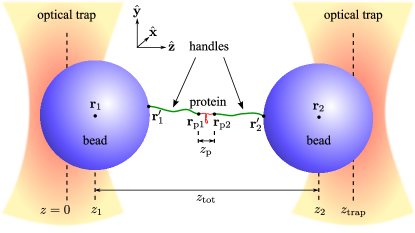
Figure 1: Dual beam optical tweezer setup for studying the equilibrium folding landscape of a single protein molecule under force.

A crucial unsolved problem is how can one construct the intrinsic free energy profile of a biomolecule using the measured folding trajectories in the presence of beads and handles (the total separation $z_{\text{tot}}(t)$ in Fig. 1 as a function of time $t$). Here, we solve this problem using a rigorous theoretical procedure. Besides $z_{\text{tot}}(t)$, the only input needed in our theory are the bead radii, the trap strengths and positions, and handle characteristics such as the contour length, the persistence length, and the elastic stretch modulus. The output is the intrinsic free energy as a function of the biomolecular extension ($z_{\text{p}}$ in Fig. 1) in the constant force ensemble.

We validate our approach using two systems: (i) a generalized Rouse model (GRM) hairpin Hyeon08 , which has an analytically solvable double-well energy landscape under force; this allows a direct test of the method; (ii) a double-stranded coiled-coil protein based on the yeast transcriptional factor GCN4 leucine zipper domain, whose folding landscape was studied using a LOT experiment Gebhardt10 . We first use coarse-grained molecular simulations to obtain the intrinsic free energy landscape of the isolated protein at a constant force. We then simulate mechanical folding trajectories using the full LOT setup, from which we quantitatively recover the intrinsic free energy landscape of GCN4, thus further establishing the efficacy of our theory. Finally, we apply our theory to experimentally generated data, and show that we can get reliable estimates for the protein energy profile independent of the optical trap parameters.

I Results

I.1 Theory for constructing the intrinsic protein folding landscape from measurements

In a dual beam optical tweezer setup (Fig. 1) the protein is covalently connected to double-stranded DNA handles that are attached to glass or polystyrene beads in two optical traps. For small displacements of the beads from the trap centers Greenleaf05 , the trap potentials are harmonic, with strengths $k_{x}=k_{z}\equiv k_{\text{trap}}$ along the lateral plane, and a weaker axial strength $k_{y}=\alpha k_{\text{trap}}$, where $\alpha<1$ Neuman04 . For simplicity, we take both traps to have equal strengths, though our method can be generalized to an asymmetric setup. The trap centers are separated from each other along the $\hat{\mathbf{z}}$ axis, with trap 1 at $z=0$ and trap 2 at $z=z_{\text{trap}}$. As the bead-handle-protein (bhp) system fluctuates in equilibrium, the positions of the bead centers, $\mathbf{r}_{1}(t)$ and $\mathbf{r}_{2}(t)$, vary in time. We assume that the experimentalist can collect a time series of the $z$ components of the bead positions, $z_{1}(t)$ and $z_{2}(t)$. Denote the mean of each time series as $\bar{z}_{1}$ and $\bar{z}_{2}$. We assume that the trap centers are sufficiently far apart that the whole system is under tension, which implies that the mean bead displacements are non-zero, $\bar{z}_{1}=z_{\text{trap}}-\bar{z}_{2}=\bar{F}/k_{\text{trap}}>0$, where $\bar{F}$ is the mean tension along $\hat{\mathbf{z}}$. We focus on the case where there is no feedback mechanism to maintain a constant force, so the instantaneous tension in the system changes as the total end-to-end extension component $z_{\text{tot}}(t)\equiv z_{2}(t)-z_{1}(t)$ [Fig. 1] varies. Though we choose one particular passive setup, the theory can be adapted to other types of passive optical tweezer systems Greenleaf05 ; Woodside06 , where the force is approximately constant (in which case we could skip the transformation into the constant-force ensemble described below). The mean tension $\bar{F}$, a measure of the overall force scale, can be tuned at the start of the experiment by making the trap separation $z_{\text{trap}}$ larger (leading to higher $\bar{F}$) or smaller (leading to lower $\bar{F}$). Because $\bar{F}=k_{\text{trap}}(z_{\text{trap}}-\bar{z}_{\text{tot}})/2$, the precise relationship between $z_{\text{trap}}$ and $\bar{F}$ requires knowing the mean total extension $\bar{z}_{\text{tot}}$, which depends among other things on the details of the energy landscape. Hence, we cannot in general calculate beforehand what $\bar{F}$ will be for a given $z_{\text{trap}}$. However, one of the advantages of our approach is that we can combine data from different experimental runs (each having a different $z_{\text{trap}}$ and $\bar{F}$) to accurately construct the protein free energy profile. This combination is carried out through the weighted histogram analysis method (WHAM) Ferrenberg89 (see Supplementary Information (SI) for details), in a spirit similar to earlier work in the context of optical tweezers Shirts08 ; Messieres11 . We first solve the problem of obtaining the protein landscape based on a single observed trajectory of bead-to-bead separations specified as $z_{\text{tot}}$ as a function of $t$.

The key quantity in the construction procedure is ${\cal P}_{\text{tot}}(z_{\text{tot}})$, the equilibrium probability distribution of $z_{\text{tot}}$ within the external trap potential, which can be directly derived from the experimental time series. The imperfect nature of the measured data, due to noise and low-pass filtering effects in the recording apparatus, will distort ${\cal P}_{\text{tot}}(z_{\text{tot}})$, but we have developed a technique to model and approximately correct for these issues (see Finite Bandwidth Scaling (FBS) in the Methods). Once we have an experimental estimate for ${\cal P}_{\text{tot}}(z_{\text{tot}})$, the objective is to find $\tilde{\cal P}_{\text{p}}(z_{\text{p}};F_{0})$, the intrinsic distribution of the protein end-to-end extension component $z_{\text{p}}$ at some constant force $F_{0}$, whose value we are free to choose. (We will use tilde notation to denote probabilities in the constant-force ensemble.) The intrinsic protein free energy profile is $\tilde{\cal F}_{\text{p}}(z_{\text{p}};F_{0})=-k_{B}T\ln\tilde{\cal P}_{\text{p}}(z_{\text{p}};F_{0})$. The procedure, obtained from rigorous theoretical underpinnings described in detail in the SI, consists of two steps:

1. Transformation into the constant-force ensemble. Given ${\cal P}_{\text{tot}}(z_{\text{tot}})$, we obtain the total system end-to-end distribution at a constant $F_{0}$ using,

   $$\begin{split}&\tilde{\cal P}_{\text{tot}}(z_{\text{tot}};F_{0})\\ &\>=C^{-1}e^{\beta F_{0}z_{\text{tot}}+\frac{1}{4}\beta k_{\text{trap}}(z_{\text{trap}}-z_{\text{tot}})^{2}}{\cal P}_{\text{tot}}(z_{\text{tot}}),\end{split}$$ (1)

   where $\beta=1/k_{B}T$ and $C$ is a normalization constant. The equation above applies in the case of a single experimental trajectory at a particular trap separation $z_{\text{trap}}$.

2. Extraction of the intrinsic protein distribution. In the constant-force ensemble, $\tilde{\cal P}_{\text{tot}}=\tilde{\cal P}_{\text{b}}\ast\tilde{\cal P}_{\text{h}}\ast\tilde{\cal P}_{\text{p}}\ast\tilde{\cal P}_{\text{h}}\ast\tilde{\cal P}_{\text{b}}$, relates the total end-to-end fluctuations $\tilde{\cal P}_{\text{tot}}(z_{\text{tot}};F_{0})$ to the end-to-end distributions for the individual components $\tilde{\cal P}_{\alpha}(z_{\alpha};F_{0})$, where $\alpha$ denotes bead (b), handle (h), or protein (p), and $\ast$ is a 1D convolution operator. For the beads, “end-to-end” refers to the extension between the bead center and the handle attachment point, projected along $\hat{\mathbf{z}}$. In Fourier space the convolution has the form:

   $$\begin{split}\tilde{\cal P}_{\text{tot}}(k;F_{0})&=\tilde{\cal P}_{\text{b}}^{2}(k;F_{0})\tilde{\cal P}^{2}_{\text{h}}(k;F_{0})\tilde{\cal P}_{\text{p}}(k;F_{0})\\ &\equiv\tilde{\cal P}_{\text{bh}}(k;F_{0})\tilde{\cal P}_{\text{p}}(k;F_{0}),\end{split}$$ (2)

   where $\tilde{\cal P}_{\alpha}(k;F_{0})$ is the Fourier transform of $\tilde{\cal P}_{\alpha}(z_{\alpha};F_{0})$. Here $\tilde{\cal P}_{\text{bh}}$, which is the result of convolving all the bead and handle distributions, acts as the main point spread function relating the intrinsic protein distribution $\tilde{\cal P}_{\text{p}}$ to $\tilde{\cal P}_{\text{tot}}$. Since $\tilde{\cal P}_{\text{bh}}$ can be modeled from a theoretical description of the handles and beads, we can solve for $\tilde{\cal P}_{\text{p}}$ using Eq. (2) and hence find $\tilde{\cal F}_{\text{p}}$, the intrinsic free energy profile of the protein.

The derivation of the procedure (given in the SI, along with technical aspects of its numerical implementation) shows the conditions under which the two step method works. The mathematical approximation underlying step 1 becomes exact if either of the following hold: (i) $k_{x}=k_{y}=0$; (ii) the full 3D total system end-to-end probability is separable into a product of distributions for longitudinal ($\hat{\mathbf{z}}$) and transverse ($\hat{\mathbf{x}}$, $\hat{\mathbf{y}}$) components. In general, condition (ii) is not physically sensible Hyeon08 . However, if $\bar{\rho}_{\text{tot}}$ is the typical length scale describing transverse fluctuations, then condition (i) is approximately valid when $\beta k_{\text{trap}}\bar{\rho}_{\text{tot}}^{2}\ll 1$. If this condition breaks down, accurate construction of the intrinsic energy landscape cannot be performed without knowledge of the transverse behavior. However, in the simulation and experimental results below, the force scales are such that transverse fluctuations are small, $\bar{\rho}_{\text{tot}}\sim{\cal O}(1\;\text{nm})$, so to ensure condition (i) is met, we require that $k_{\text{trap}}\ll k_{B}T/\bar{\rho}_{\text{tot}}^{2}=4.1$ pN/nm at $T=298$ K. We use the experimental value $k_{\text{trap}}=0.25\;\text{pN}/\text{nm}$ in our test cases Gebhardt10 , which is well under the upper limit. In principle, one can choose any $F_{0}$, the force value of the constant force ensemble where we carry out the analysis. In practice, $F_{0}$ should be chosen from among the range of forces that is sampled in equilibrium during the actual experiment, since this will minimize statistical errors in the final constructed landscape. For example, setting $F_{0}=\bar{F}$, the mean tension, is a reasonable choice.

Step 2 depends on knowledge of $\tilde{\cal P}_{\text{bh}}(k;F_{0})$, and thus the individual constant-force distributions of the beads and the handles in Fourier space. The point spread function is characterized by: the bead radius $R_{b}$, the handle contour length $L$, the handle persistence length $l_{p}$, and the handle elastic stretching modulus $\gamma$. In $\tilde{\cal P}_{\text{h}}$ we also include the covalent linkers which attach the handles to the beads and protein. If we model these linkers as short, stiff harmonic springs, we have two additional parameters: the linker stiffness $\kappa$ and natural length $\ell$. Using the extensible semiflexible chain as a model for the handles, we exploit an exact mapping between this model and the propagator for the motion of a quantum particle on the surface of a unit sphere Kierfeld04 to calculate the handle Fourier-space distribution to arbitrary numerical precision. Together with analytical results for the bead and linker distributions, we can thus directly solve for $\tilde{\cal P}_{\text{bh}}(k;F_{0})$. To verify that the analytical model for the point-spread function can accurately describe handle/bead fluctuations over a range of forces, we have analyzed data from control experiments on a system involving only dsDNA handles attached to beads, where ${\cal P}_{\text{tot}}={\cal P}_{\text{bh}}$ (SI). The theory simultaneously fits results for several experimental quantities measured on the same system: the distributions $\tilde{\cal P}_{\text{bh}}$ derived from three different trap separations, corresponding to mean forces $F_{0}=9.4-12.7$ pN, and a force-extension curve. The accuracy of the model $\tilde{\cal P}_{\text{bh}}$ is $\approx 1-3\%$, within the experimental error margins.

I.2 Robustness of the theory validated by application to an exactly soluble model

We first apply the theory to a problem for which the intrinsic free energy profiles at arbitrary force are known exactly. The generalized Rouse model (GRM) hairpin (see SI for details) is a two-state folder whose full 3D equilibrium end-to-end distributions are analytically solvable. A representative GRM distribution $\tilde{\cal P}_{\text{GRM}}$ at $F_{0}=11.9$ pN is plotted in Fig. 2(a). Since $\tilde{\cal P}_{\text{GRM}}$ is cylindrically symmetric, the top panel shows a projection onto the $(\rho=\sqrt{x^{2}+y^{2}},z)$ plane, while the bottom panel shows the further projection onto the $z$ coordinate. The two peaks correspond to the native (N) state at small $z$, and the unfolded (U) state at large $z$. In order to model the optical tweezer system, we add handles and beads to the GRM hairpin, whose probabilities $\tilde{\cal P}_{\text{h}}$ and $\tilde{\cal P}_{\text{b}}$ (including transverse fluctuations) are illustrated in Fig. 2(b) and (c). The full 3D behavior is derived in an analogous manner to the theory mentioned above for the 1D Fourier-space distribution $\tilde{\cal P}_{\text{bh}}(k;F_{0})$ of the beads/handles; the only difference is that the transverse degrees of freedom are not integrated out. The 3D convolution of the system components, plus the optical trap contribution, gives the total distribution ${\cal P}_{\text{tot}}$ in Fig. 2(d). The bead, handle, linker, and trap parameters are listed in SI Table S1. From ${\cal P}_{\text{tot}}$ one can calculate the mean total $z$ extension and the mean tension, which in this case are $\bar{z}_{\text{tot}}=1199$ nm, $\bar{F}=k_{\text{trap}}(z_{\text{trap}}-\bar{z}_{\text{tot}})/2=11.9$ pN.

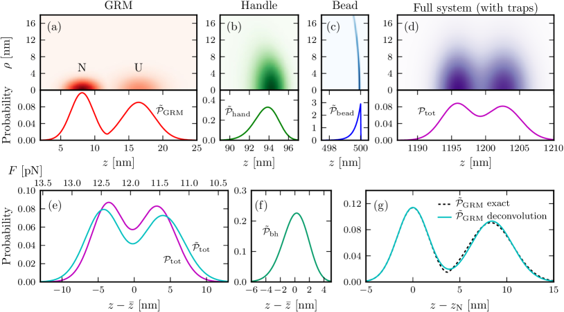
Figure 2: Generalized Rouse model (GRM) hairpin in an optical tweezer setup. The first row shows the exact end-to-end distributions along $\hat{\mathbf{z}}$ for each component type in the system: a) GRM, b) dsDNA handle, c) polystyrene bead. The handle, bead and trap parameters are listed in Table S1 (GRM column). Upper panels show the probabilities projected onto cylindrical coordinates $(\rho=\sqrt{x^{2}+y^{2}},z)$, while the lower ones show the projection onto $z$ alone. (d) The result for the total system end-to-end distribution, ${\cal P}_{\text{tot}}$, derived by convolving the component probabilities and accounting for the optical traps. (e-g) The construction of the original GRM distribution $\tilde{\cal P}_{\text{GRM}}$ starting from ${\cal P}_{\text{tot}}$. (e) ${\cal P}_{\text{tot}}$ (purple) and $\tilde{\cal P}_{\text{tot}}$ (blue) as a function of $z$ on the bottom axis, measured relative to $\bar{z}$, the average extension for each distribution. For ${\cal P}_{\text{tot}}$, the upper axis shows the $z$ range translated into the corresponding trap forces $F$. After removing the trap effects, $\tilde{\cal P}_{\text{tot}}$ is the distribution for constant force $F_{0}=11.9$ pN. (f) $\tilde{\cal P}_{\text{bh}}$, describing the total probability at $F_{0}$ of fluctuations resulting from both handles and the rotation of the beads. (g) The constructed solution for $\tilde{\cal P}_{\text{GRM}}$ (solid line), obtained by numerically inverting the convolution $\tilde{\cal P}_{\text{tot}}=\tilde{\cal P}_{\text{bh}}\ast\tilde{\cal P}_{\text{GRM}}$. The exact analytical result for $\tilde{\cal P}_{\text{GRM}}$ is shown as a dashed line. $z_{\text{N}}$ is the position of the native state (N) peak.

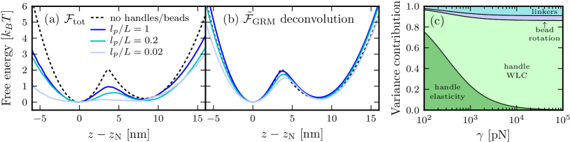
Figure 3: Effects of handle characteristics on the free energy profile of the GRM in an LOT setup. (a) The total system free energy ${\cal F}_{\text{tot}}=-k_{B}T\ln{\cal P}_{\text{tot}}$ for fixed $L=100$ nm, and varying ratios $l_{p}/L$. All the other parameters are in Table S1 (GRM column). The exact analytical free energy at $F_{0}=11.9$ pN (dashed line) for the GRM alone, $\tilde{\cal F}_{\text{GRM}}=-k_{B}T\ln\tilde{\cal P}_{\text{GRM}}$, is shown for comparison. (b) For each ${\cal F}_{\text{tot}}$ in (a), the construction of $\tilde{\cal F}_{\text{GRM}}$ at $F_{0}$, together with the exact answer (dashed line). (c) For system parameters matching the experiment (Table S1), the variance of the point spread function $\tilde{\cal P}_{\text{bh}}$ broken down into the individual handle, bead, and linker contributions. The fraction for each component is shown as a function of varying handle elastic modulus $\gamma$.

The $\mathbf{\hat{z}}$ probability projection in the bottom panel of (d) is the information accessible in an experiment, and the computation of the intrinsic distribution in the bottom panel of (a) is the ultimate goal of the construction procedure. Comparing (a) and (d), two effects of the apparatus are visible: the GRM peaks have been partially blurred into each other, and the transverse ($\rho$) fluctuations have been enhanced. The handles provide the dominant contribution to both these effects.

Figs. 2(e) through (g) illustrate the construction procedure for the GRM optical tweezer system. Panel (e) corresponds to Step 1, with a transformation of the distribution ${\cal P}_{\text{tot}}$ (whose varying force scale is shown along the top axis) into $\tilde{\cal P}_{\text{tot}}$ at constant force $F_{0}=11.9$ pN. Step 2 uses the exact $\tilde{\cal P}_{\text{bh}}$, shown in real-space in panel (f), and produces the intrinsic distribution $\tilde{\cal P}_{\text{GRM}}$, drawn as a solid line in (g). The agreement with the exact analytical result (dashed line) is extremely close, with a median error of $3\%$ over the range shown. This deviation is due to the approximation in Step 1, discussed above, as well as the numerical implementation of the deconvolution procedure.

As shown in our previous study Hyeon08 , the smaller the ratio $l_{p}/L$ for the handles, the more the features of the protein energy landscape get blurred by the handle fluctuations. Since the experimentally measured total distribution always distorts to some extent the intrinsic protein free energy profile due to the finite duration and sampling of the system trajectory, more flexible handles will exacerbate the signal-to-noise problem. To illustrate this effect, we performed Brownian dynamics simulations of the GRM in the optical tweezer setup, with handles modeled as extensible, semiflexible bead-spring chains (see SI for details). In Fig. 3(a) we compare the free energy ${\cal F}_{\text{tot}}=-k_{B}T\ln{\cal P}_{\text{tot}}$ for a fixed $L=100$ nm and a varying $l_{p}/L$, derived from the simulation trajectories, and the exact intrinsic GRM result $\tilde{\cal F}_{\text{GRM}}=-k_{B}T\ln\tilde{\cal P}_{\text{GRM}}$ at $F_{0}$. When the handles are very flexible, with $l_{p}/L=0.02$, the energy barrier between the native and unfolded states almost entirely disappears in ${\cal F}_{\text{tot}}$, with the noise making the precise barrier shape difficult to resolve. Remarkably, even with this extreme level of distortion, using our theory we still recover a reasonable estimate of the intrinsic landscape [Fig. 3(b)]. For each ${\cal F}_{\text{tot}}$ in Fig. 3(a), panel Fig. 3(b) compares the result of the construction procedure and the exact answer for $\tilde{\cal F}_{\text{GRM}}$. Clearly some information is lost as $l_{p}/L$ becomes smaller, since the $l_{p}/L=0.02$ system does not yield as accurate a result as the ones with stiffer handles. However in all cases the basic features of the exact $\tilde{\cal F}_{\text{GRM}}$ are reproduced. Thus, the theoretical-based method works remarkably well over a wide range of handle parameters. This conclusion is generally valid even when other parameters are varied (see Fig. S3 in the SI for tests at various $F_{0}$ and $k_{\text{trap}}$). The excellent agreement between the constructed and intrinsic free energy profiles for the exactly solvable GRM hairpin over a wide range of handle and trap experimental variables establishes the robustness of the theory.

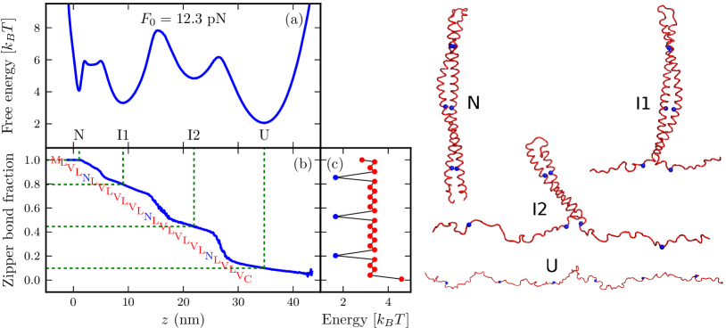
Figure 4: Intrinsic characteristics of the LZ26 leucine zipper at constant $F_{0}$, derived from SOP simulations in the absence of handles/beads. (a) LZ26 free energy $\tilde{\cal F}_{\text{p}}$ at $F_{0}=12.3$ pN vs. end-to-end extension $z$. Representative protein configurations from the four wells (N, I1, I2, U) are shown on the right, with asparagine residues colored blue. (b) The average fraction of native contacts between the two alpha-helical strands of LZ26 (the “zipper bonds”) as a function of $z$. Listed to the left of the curve are the $a$ and $d$ residues in the heptads making up the amino acid sequence for each LZ26 strand, placed according to their position along the zipper. Asparagines (N) are highlighted in blue. (c) For the residues listed in (b), the residue contact energies used in the SOP simulation (rescaled BT Betancourt99 values).

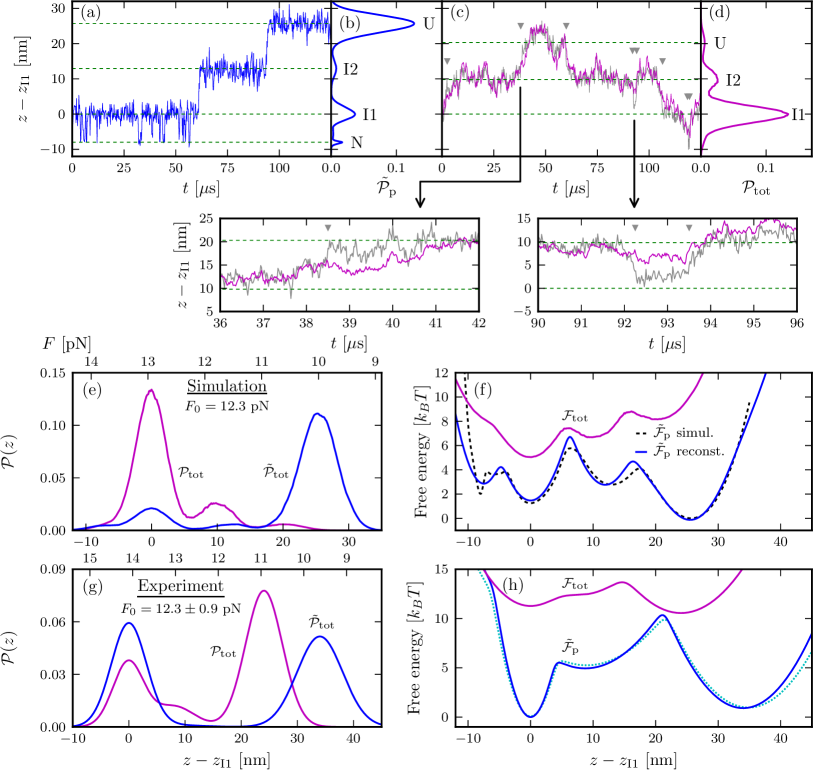
Figure 5: (a,b) A trajectory fragment and the probability distribution $\tilde{\cal P}_{\text{p}}$ from SOP simulations of the LZ26 leucine zipper at constant force $F_{0}=12.3$ pN in the absence of handles/beads. (c,d) A trajectory fragment and the total system distribution ${\cal P}_{\text{tot}}$ at $z_{\text{trap}}=503$ nm. Panel (c) shows both the total extension $z_{\text{tot}}(t)$ (purple) and the protein extension $z_{\text{p}}(t)$ (gray). Triangles mark times when the protein makes a transition between states, and the arrows point to two enlarged portions of the trajectories. In all cases the $z$-axis origin is $z_{\text{I1}}$, the peak location of the I1 intermediate state. (e-g) Leucine zipper free energy profiles extracted from time series (third row = simulation, fourth row = experiment). The first column shows the total system end-to-end distribution ${\cal P}_{\text{tot}}$, and the corresponding $\tilde{\cal P}_{\text{tot}}$ at constant force $F_{0}=12.3$ pN. In the experimental case $F_{0}=12.3\pm 0.9$ pN is the mid-point force at which the I1 and U states are equally likely. For ${\cal P}_{\text{tot}}$, $z_{\text{trap}}=503$ nm (simulation), $1553\pm 1$ nm (experiment). Force scales at the top are the range of trap forces for ${\cal P}_{\text{tot}}$. The second column shows the computed intrinsic protein free energy profiles $\tilde{\cal F}_{\text{p}}$, compared to the total system profile, ${\cal F}_{\text{tot}}$ (shifted upwards for clarity). (f) SOP simulations for the protein alone at constant $F_{0}$ provide a reference landscape, drawn as a dashed line. (h) The dashed curve is the reconstructed $\tilde{\cal F}_{\text{p}}$ at the mid-point force $F_{0}=12.1\pm 0.9$ pN, from a second, independent experimental trajectory, with $z_{\text{trap}}=1547\pm 1$ nm. The $\tilde{\cal F}_{\text{p}}$ curves have a median uncertainty of $0.4$ $k_{B}T$ over the plotted range (see SI for error analysis).

I.3 Intrinsic folding landscape of a simulated leucine zipper

To demonstrate that the theory can be used to produce equilibrium intrinsic free energy profiles with multiple states from mechanical folding trajectories, we performed simulations of a protein in an optical tweezer setup. The simulations were designed to mirror the single-molecule experiment reported in Ref. Gebhardt10 , and to this end we studied a coiled-coil, LZ26 Bornschlogl06 , based on three repeats of the leucine zipper domain from the yeast transcriptional factor GCN4 OShea91 (see Methods). The simple linear unzipping of the two strands of LZ26 allows us to map the end-to-end extension to the protein configuration. Furthermore, the energy heterogeneity of the native bonds that form the “teeth” of the zipper leads to a non-trivial folding landscape with at least two intermediate states Bornschlogl06 ; Bornschlogl08 ; Gebhardt10 . The more complex landscape of LZ26 thus provides an additional stringent test of the proposed theory.

The native (N) structure of LZ26 is illustrated on the right in Fig. 4 (from a simulation snapshot), with the two alpha-helical strands running from N-terminus at the bottom to C-terminus at the top. In the experiment a handle is attached to the N-terminus of each strand, and this is where the strands begin to unzip under applied force. To prevent complete strand separation, the C-termini are cross-linked through a disulfide bridge between two cysteine residues. Each alpha-helix coil consists of a series of seven-residue heptad repeats, with positions labeled a through g. For the leucine zipper the a and d positions are the “teeth”, consisting of mostly hydrophobic residues (valine and leucine) which have strong non-covalent interactions with their counterparts on the other strand. The exceptions to the hydrophobic pattern are the three hydrophilic asparagine residues in $a$ positions on each strand (marked in blue in the structure snapshots on the right of Fig. 4). As has been seen experimentally Bornschlogl06 ; Gebhardt10 (and shown below through simulations), the weaker interaction of these asparagine pairs is crucial in determining the properties of the intermediate folding states, a point we will return to in more detail in the Discussion.

In analyzing the LZ26 leucine zipper system, we performed coarse-grained simulations using the Self-Organized Polymer (SOP) model Hyeon06 (full details in the SI, with selected parameters summarized in Table S1). The intrinsic free energy profile $\tilde{\cal F}_{\text{p}}=-k_{B}T\ln\tilde{\cal P}_{\text{p}}$ at $F_{0}=12.3$ pN is shown in Fig. 4(a). The four prominent wells in $\tilde{\cal F}_{\text{p}}$ as a function of $z_{\text{p}}$ correspond to four stages in the progressive unzipping of LZ26. At $F_{0}=12.3$ pN all the states are populated, and the system fluctuates in equilibrium between the wells. The transition barrier between N and I1 exhibits a shallow dip that may correspond to an additional, very transiently populated intermediate. Since this dip is much smaller than $k_{B}T$, we do not count it as a distinct state.

Like in the GRM example, adding the optical tweezer apparatus to the SOP simulation significantly distorts the measured probability distributions. In the first row of Fig. 5 sample simulation trajectory fragments are shown both for the protein-only case [Fig. 5(a)] at constant force $F_{0}=12.3$ pN, and within the full optical tweezer system [Fig. 5(c)] with $z_{\text{trap}}=503$ nm. For the latter case we plot both $z_{\text{tot}}(t)$ (purple) and $z_{\text{p}}(t)$ (gray), allowing us to see how the bead separation tracks changes in the protein extension. The probability distributions $\tilde{\cal P}_{\text{p}}$ and ${\cal P}_{\text{tot}}$ are plotted in Fig. 5(b) and (d) respectively. In Fig. 5(e), the distribution ${\cal P}_{\text{tot}}$ within the optical tweezer system is plotted for $z_{\text{trap}}=503$ nm. Though we only illustrate this particular $z_{\text{trap}}$ value, $\approx 260$ trajectories are generated at different $z_{\text{trap}}$ and combined together using WHAM Ferrenberg89 (see SI) to produce a single $\tilde{\cal P}_{\text{tot}}$ at a constant force $F_{0}=12.3$ pN [Fig. 5(e)]. We can then use our theoretical method to recover the protein free energy $\tilde{\cal F}_{\text{p}}$ [Fig. 5(f)]. Despite numerical errors due to limited statistical sampling (both in the protein-only and total system runs), there is remarkable agreement between the constructed result and $\tilde{\cal F}_{\text{p}}$ derived from protein-only simulations. This is particularly striking given that the total system free energy ${\cal F}_{\text{tot}}(z_{\text{tot}})=-k_{B}T\ln{\cal P}_{\text{tot}}(z_{\text{tot}})$, plotted for comparison in panels (f), shows how severely the handles/beads blur the energy landscape, reducing the energy barriers to a degree that the N state is difficult to resolve. The signature of N in ${\cal F}_{\text{tot}}(z_{\text{tot}})$ is a slight change in the curvature at higher energies on the left of the I1 well. However despite this, we still recover a basin of attraction representing the N state in the constructed $\tilde{\cal F}_{\text{p}}$. Overall, the results in (f) show that our theory can accurately produce the intrinsic free energy profiles using only the simulated folding trajectories as input, thus proving a self-consistency check of the method for a system with multiple intermediates.

I.4 Folding landscape of the leucine zipper from experimental trajectories

As a final test of the efficacy of the theory we used the experimental time series data Gebhardt10 to obtain $\tilde{\cal F}_{\text{p}}$. The data consists of two independent runs with the LZ26 leucine zipper, using the same handle/bead parameters for each run (see Table S1), but at different trap separations $z_{\text{trap}}$. We project the deconvolved landscape from each trajectory onto the mid-point force $F_{0}$ where the two most populated states (I1 and U) have equal probabilities in $\tilde{\cal P}_{\text{p}}$. The values of $F_{0}$ derived from the two runs are the same within error bounds: $12.3\pm 0.9$ and $12.1\pm 0.9$ pN. The detailed deconvolution steps are shown for one run in the last row of Fig. 5, and the final result, the intrinsic free energy profile $\tilde{\cal F}_{\text{p}}$, is shown for both runs in Fig. 5(h) (solid and dotted blue curves respectively). Accounting for error due to finite trajectory length and uncertainties in the apparatus parameters, the median total uncertainty in each of the reconstructed landscapes is about $0.4$ $k_{B}T$ in the $z$ range shown (see SI for full error analysis). The landscapes from the two independent runs have a median difference of $0.3$ $k_{B}T$, and hence the method gives consistent results between runs, up to a small experimental uncertainty, an important test of its practical utility. The reproducibility of $\tilde{\cal F}_{\text{p}}$ is a testament to the stability of the dual optical tweezer setup, allowing us to sample extensively from the energy landscape: each trajectory lasted for more than 100 s, and thus collected $\sim{\cal O}(10^{2}-10^{5})$ of the various types of transitions between protein states (the slowest transition, $\text{U}\to\text{I2}$, occurred on time scales of $0.4-0.6$ s).

Comparison between the experimental $\tilde{\cal F}_{\text{p}}$ in panel (h) and the simulation result in (f) reveals a notable difference: the landscape constructed using the experimental data does not have four identifiable basins. The N state may not be discernible in the experiment because of the limited resolution of the apparatus (see below). The spacing between the I1 and I2 wells is similar in the simulation and experiment ($\approx 9-13$ nm), but that between I2 and U is $\approx 13$ nm in the simulation versus 25 nm in the experiment. This is likely due to a larger helix content in the unfolded state for the simulation case.

II Discussion

II.1 Origins of the variance in the point spread function

Our theory for the point spread function $\tilde{P}_{\text{bh}}$ can be used to understand the interplay of physical effects that relate the intrinsic protein distribution to the total system. To quantify the various contributions to $\tilde{P}_{\text{bh}}$, we calculated its variance. Since variances of probability distributions combine additively upon convolution, we break down the variance of $\tilde{P}_{\text{bh}}$ into the individual bead, handle, and linker contributions. Fig. 3(c) shows the fraction of the variance associated with each component as a function of the handle elastic stretching modulus $\gamma$ at $F_{0}=12.3$ pN, with $R_{b}=500$ nm, $L=188$ nm, $l_{p}=20$ nm (the approximate experimental parameters from Ref. Gebhardt10 ). For any given value of $\gamma$, the height of each of the four colored slices represents four fractions. Though not directly measured in Ref. Gebhardt10 , we have assumed $\kappa=200$ kcal/mol$\cdot$nm², $\ell=1.5$ nm for the linkers. The handle contribution is itself broken down into the “elastic” part, defined as the extra variance due to the finite stretching modulus $\gamma$, compared to an inextensible ($\gamma\to\infty$) worm-like chain (WLC), and the remainder, which we call the WLC part. For the case of Ref. Gebhardt10 , $\gamma=400$ pN. Since the length extension relative to the WLC result is $\approx F_{0}/\gamma$, we expect finite handle extensibility to play a small role. However, the elastic contribution to the total $\tilde{\cal P}_{\text{bh}}$ variance at this $\gamma$ is 43%, comparable to the WLC contribution of 48%. Hence, in predicting $\tilde{\cal P}_{\text{bh}}$ correctly it is important to account for both the bending rigidity and elasticity of the handles, which are exactly modeled in our approach.

II.2 Nature and location of the intermediate states in the leucine zipper energy landscape

The folding landscape of LZ26 is apparently closely related to the pattern of residue-residue contact energies between the two strands of the zipper Bornschlogl06 ; Bornschlogl08 ; Gebhardt10 . SOP simulations give us a detailed picture of this relationship. The average fraction of intact inter-strand (“zipper”) bonds vs. extension $z$, in Fig. 4(b) is a monotonic curve, starting with the fully closed structure on top (N state, bond fraction near 1) to the fully open structure at the bottom (U state, bond fraction near 0). Listed along this curve are the individual residues at the $a$ and $d$ positions of the heptads in the sequence. Several features stand out: the transition barriers between the states show a steeper rate of zipper bond unraveling compared to the well regions. The change of slope from steep to more gradual descent occurs near the location of the asparagine residues in the sequence, and the the well minima of I1, I2, and U occur one or two residues after the asparagines. The correlation between well minima locations and asparagines agrees with the experimental landscape Gebhardt10 , underscoring the importance of the weak, hydrophilic asparagine bonds that interrupt the hydrophobic valine/leucine pattern at the a/d positions. The sequence of rescaled BT Betancourt99 energies used for the a/d native contacts is plotted in Fig. 4(c). The a/d bonds are all $>2.8$ $k_{B}T$, except for the asparagines, which are less stable at $1.7$ $k_{B}T$.

II.3 Instrumental noise filtering, and the limits of the theoretical approach

The difference in the number of wells in the simulation and experimental free energy landscapes of the leucine zipper is related to finite time and spatial resolution. The measured time series is subject to noise (environmental vibrations of the optical elements, detector shot noise), as well as low-pass filtering due to “parasitic” effects in the photodiodes and the nature of the electronic amplification circuits vonHansen12 . The standard experimental protocol often involves additional low-pass filtering as a way of removing noise and smoothing trajectories: for the leucine zipper every five data points (originally recorded at 10 $\mu$s intervals) are averaged together during collection to give a time step of 50 $\mu$s Gebhardt10 ; in other cases similar effects are achieved using Bessel filters Yu12 . Noise broadens the measured distribution of bead separations, while low-pass filtering narrows it. We developed the FBS technique (Methods and SI), based on the details of the specific apparatus used in the experiment, to estimate and correct for the distortions. For our system, the FBS theory provides an excellent description, as we have verified in tests using both numerical simulations and experimental data (with and without the additional filtering).

However the FBS theory can only apply corrections to peaks (i.e. distinct protein states) that we observe in the measured probability distributions. There is the possibility of protein states leaving no discernible signature in the recorded distribution. The N state in the leucine zipper is only connected to the I1 state in the folding pathway. In the simulations, where the N state is directly observed, it has short mean lifetimes ($\lesssim 6$ $\mu$s in the studied force range), and the $\text{N}\leftrightarrow\text{I1}$ change involves the shortest mean extension difference ($\approx 8$ nm) among all the transitions. If the N state in the actual protein has similar properties, it could be impossible to resolve it in the experimental data for two different reasons: (i) Regardless of any additional filtering, the intrinsic low-pass characteristics of the apparatus filter out states with very short lifetimes. For our LOT setup, the effective low-pass filter time-scale for the detectors/electronics is $\tau_{f}\approx 7$ $\mu$s (SI), which is at the cutting edge of current technology. Thus, states with lifetimes $\lesssim\tau_{f}$ will not appear as distinct peaks in the measured distribution. (ii) Independent of the filtering issues in detection/recording, environmental background noise in the time series also poses a problem, particularly since we measure bead displacements, and these have signal amplitudes at high frequencies that are generally attenuated compared to the intrinsic amplitudes of the protein conformational changes. The reason for this is that the beads have much larger hydrodynamic drag than dsDNA handles or proteins, and their characteristic relaxation times $\tau_{r}$ in the optical traps may be comparable to or larger than the lifetime of a particular protein state. The bead cannot fully respond to force changes on time scales shorter than its relaxation time Manosas07BJ . For example, $\tau_{r}\approx 20$ $\mu$s in the leucine zipper experiment. If the lifetime of the N state at a particular force is much smaller than $\tau_{r}$, protein transitions from I1$\to$N$\to$I1 will generally occur before the bead can relax into the N state equilibrium position. If the bead displacements associated with these transitions are smaller than the noise amplitude in the time series, the entire excursion to the N state will be lost to the noise.

We can illustrate the finite response time of the bead using simulations where resolution is not limited by noise or apparatus filtering, allowing us to illustrate the relationship between $z_{\text{tot}}(t)$ and $z_{\text{p}}(t)$, compared in two different trajectory fragments in Fig. 5(c). Triangles in the figure indicate times where the protein makes a transition between states. Changes in protein extension during these transitions are very rapid, and the bead generally mirrors these changes with a small time lag, as seen in the enlarged trajectory interval at $t=36-42$ $\mu$s. When the protein makes sharp, extremely brief excursions (like a visit to the N state from I1 in the enlarged interval $t=90-96$ $\mu$s), the corresponding changes in bead separation are smaller and much less well-defined. In the presence of noise, such tiny changes would be obscured.

Thus, we surmise that the N state is not observable due to some combination of apparatus filtering, noise, and finite bead response time. Hence, the theory applied to the experimental data produces a landscape with only I1, I2, and U wells, as opposed to the four wells produced from the simulation data. Our labeling of the basins in the landscape agrees with the earlier state identification Gebhardt10 , and provides an explanation for why the N state was not resolved.

III Conclusions

Extraction of the energy landscape of biomolecules using LOT data is complicated because accurate analysis depends on correcting for distortions due to system components on the measured result. We have solved this problem completely by developing a theoretically-based construction method that accounts for these factors. Through an array of tests involving an analytically solvable hairpin model, coarse-grained protein simulations, and experimental data, we have demonstrated the robustness of the technique in a range of realistic scenarios. The method works for arbitrarily complicated landscapes, as demonstrated by the analysis of the leucine zipper experimental data, producing consistent results when the same protein is studied under different force scales.

IV Materials and Methods

IV.1 Finite Bandwidth Scaling (FBS)

Probability distributions derived from experimental time series of bead-bead separations are corrupted by noise, low-pass filtering due to the apparatus, and in some cases additional filtering due to the data processing protocol. We developed FBS theory to model and correct for these effects (see SI for details), using information encoded in time series autocorrelations, together with earlier spectral characterization of the dual trap optical tweezer detector and electronic systems vonHansen12 . All the experimental distributions ${\cal P}_{\text{tot}}$ in the main text were first processed by FBS.

IV.2 Leucine zipper

We use a variant of the coarse-grained self-organized polymer (SOP) model Hyeon06 ; Mickler07PNAS , where each of the 176 residues in LZ26 is represented by a bead centered at the $C_{\alpha}$ position (see SI for details.) The $\alpha$-helical secondary structure is stabilized by interactions which mimic $(i,i+4)$ hydrogen bonding Denesyuk11 . We use residue-dependent energies for tertiary interactions Betancourt99 .

IV.3 Simulations

We simulate (see SI for details) trajectories for both the protein alone and the full optical tweezer setup using an overdamped Brownian dynamics (BD) algorithm Ermak78 . The handles used in the LOT setup [Fig. 1] are modeled as semiflexible chains.

Supplementary information for “From mechanical folding trajectories to intrinsic energy landscapes of biopolymers”
Michael Hinczewski, J. Christof M. Gebhardt, Matthias Rief, and D. Thirumalai

Table S1: Parameters used in the GRM model and SOP simulation of the LZ26 leucine zipper, together with the corresponding quantities from two experimental runs Gebhardt10

Parameter	GRM	SOP Simulation	Experiment
Bead: $R_{b}$ (nm)	500	100	500$\pm$25
Trap: $z_{\text{trap}}$ (nm)	1294	483 – 543	1553$\pm$1, 1547$\pm$1
Trap: $k_{\text{trap}}$ (pN/nm)	0.25	0.25	0.25$\pm$0.03, 0.27$\pm$0.03
Trap: $\alpha$	1/3	1/3	unknown
Handle: $L$ (nm)	100	100	188$\pm$2
Handle: $l_{p}$ (nm)	20	20	20$\pm$2
Handle: $\gamma$ (pN)	2780	2780	400$\pm$40
Linker: $\kappa$ (kcal/mol$\cdot$nm2)	200	200	200
Linker: $\ell$ (nm)	1.5	1.5	1.5

I Theory for free energy construction from mechanical folding time series

I.1 Optical trap Hamiltonian

We begin with the Hamiltonian for the beads in the traps (Fig. 1 in the main text), which allows us to introduce the relevant variables of the system. If the displacements of the beads from the trap centers are small ($<100$ nm for a laser of 1064 nm wavelength and bead radii $\sim{\cal O}(100\;\text{nm})$ Greenleaf05 ), the trap Hamiltonian can be approximately written as:

$${\cal H}_{\text{trap}}(\mathbf{r}_{1},\mathbf{r}_{2})=\frac{1}{2}k_{x}(x_{1}^{2}+x_{2}^{2})+\frac{1}{2}k_{y}(y_{1}^{2}+y_{2}^{2})+\frac{1}{2}k_{z}\left[z_{1}^{2}+(z_{\text{trap}}-z_{2})^{2}\right],$$ (S1)

where $\mathbf{r}_{i}=(x_{i},y_{i},z_{i})$ is the position of the $i$th bead center, $k_{x}$, $k_{y}$, $k_{z}$ are the trap strengths along each coordinate direction, and the two traps are positioned at $z=0$ and $z=z_{\text{trap}}$ respectively. Given the cylindrical symmetry of the optical traps around the $\hat{\mathbf{y}}$ axis, we take $k_{x}=k_{z}\equiv k_{\text{trap}}$ and $k_{y}=\alpha k_{\text{trap}}$, where the weaker axial trapping is reduced by a factor $\alpha<1$ Neuman04 . We assume both traps have equal strengths, though our method can be generalized to an asymmetric configuration, where the two traps have different strengths $k_{\text{trap,1}}\neq k_{\text{trap,2}}$. In this case the reconstruction procedure derived below is valid with the substitution $k_{\text{trap}}=2k_{\text{trap,1}}k_{\text{trap,2}}/(k_{\text{trap,1}}+k_{\text{trap,2}})$.

We rewrite the Hamiltonian in Eq. (S1) by defining a total end-to-end coordinate $\mathbf{r}_{\text{tot}}\equiv\mathbf{r}_{2}-\mathbf{r}_{1}=(x_{\text{tot}},y_{\text{tot}},z_{\text{tot}})$, and a total center-of-mass coordinate $\mathbf{R}_{\text{tot}}\equiv\mathbf{r}_{2}+\mathbf{r}_{1}=(X_{\text{tot}},Y_{\text{tot}},Z_{\text{tot}})$. In terms of these variables, ${\cal H}_{\text{trap}}$ becomes:

$$\begin{split}{\cal H}_{\text{trap}}(\mathbf{r}_{1},\mathbf{r}_{2})&={\cal H}^{\text{cm}}_{\text{trap}}(\mathbf{R}_{\text{tot}})+{\cal H}^{\text{ee}}_{\text{trap}}(\mathbf{r}_{\text{tot}}),\\ {\cal H}^{\text{cm}}_{\text{trap}}(\mathbf{R}_{\text{tot}})&=\frac{1}{4}k_{x}X_{\text{tot}}^{2}+\frac{1}{4}k_{y}Y_{\text{tot}}^{2}+\frac{1}{4}k_{z}(z_{\text{trap}}-Z_{\text{tot}})^{2},\\ {\cal H}^{\text{ee}}_{\text{trap}}(\mathbf{r}_{\text{tot}})&=\frac{1}{4}k_{x}x_{\text{tot}}^{2}+\frac{1}{4}k_{y}y_{\text{tot}}^{2}+\frac{1}{4}k_{z}(z_{\text{trap}}-z_{\text{tot}})^{2}.\end{split}$$ (S2)

The variables $z_{\text{tot}}$ and $z_{\text{trap}}$ are explicitly labeled in Fig. 1 of the main text.

I.2 Equilibrium distribution of the system

The equilibrium probability ${\cal P}_{\text{tot}}(\mathbf{R}_{\text{tot}},\mathbf{r}_{\text{tot}})$ of finding the beads at positions with a given $\mathbf{R}_{\text{tot}}$ and $\mathbf{r}_{\text{tot}}$ can be expressed as:

$${\cal P}_{\text{tot}}(\mathbf{R}_{\text{tot}},\mathbf{r}_{\text{tot}})=Ae^{-\beta{\cal H}^{\text{cm}}_{\text{trap}}(\mathbf{R}_{\text{tot}})-\beta{\cal H}^{\text{ee}}_{\text{trap}}(\mathbf{r}_{\text{tot}})}{\cal Q}_{\text{tot}}(\mathbf{r}_{\text{tot}}),$$ (S3)

where $\beta=1/k_{B}T$, $A$ is a normalization constant, and ${\cal Q}_{\text{tot}}(\mathbf{r}_{\text{tot}})$ is the equilibrium probability of the total bead-handle-protein system having bead separation $\mathbf{r}_{\text{tot}}$ in the absence of the external trapping potential or any applied force. By translational symmetry ${\cal Q}_{\text{tot}}$ is independent of the center-of-mass coordinates, and by rotational symmetry ${\cal Q}_{\text{tot}}(\mathbf{r}_{\text{tot}})={\cal Q}_{\text{tot}}(|\mathbf{r}_{\text{tot}}|)$. Thus, if we introduce cylindrical coordinates $\mathbf{r}_{\text{tot}}=(\rho_{\text{tot}},\phi_{\text{tot}},z_{\text{tot}})$, where $\rho_{\text{tot}}=\sqrt{x_{\text{tot}}^{2}+y_{\text{tot}}^{2}}$, $\phi_{\text{tot}}=\tan^{-1}(y_{\text{tot}}/x_{\text{tot}})$, there is no angular dependence, so that ${\cal Q}_{\text{tot}}(\mathbf{r}_{\text{tot}})={\cal Q}_{\text{tot}}(\rho_{\text{tot}},z_{\text{tot}})$. We are ultimately interested in the marginal probability ${\cal P}_{\text{tot}}(z_{\text{tot}})$, which can be derived from the experimental time series and forms the starting point of our theoretical procedure to obtain the desired free energy profile. We obtain ${\cal P}_{\text{tot}}(z_{\text{tot}})$ from ${\cal P}_{\text{tot}}(\mathbf{R}_{\text{tot}},\mathbf{r}_{\text{tot}})$ by integrating over the $\mathbf{R}_{\text{tot}}$, $\rho_{\text{tot}}$ and $\phi_{\text{tot}}$ degrees of freedom:

$$\begin{split}{\cal P}_{\text{tot}}(z_{\text{tot}})&\equiv\int\rho_{\text{tot}}\,d\rho_{\text{tot}}\,d\phi_{\text{tot}}\,d\mathbf{R}_{\text{tot}}\,{\cal P}_{\text{tot}}(\mathbf{R}_{\text{tot}},\mathbf{r}_{\text{tot}})\\ &=B\int\rho_{\text{tot}}\,d\rho_{\text{tot}}\,d\phi_{\text{tot}}\,e^{-\beta{\cal H}^{\text{ee}}_{\text{trap}}(\rho_{\text{tot}},\phi_{\text{tot}},z_{\text{tot}})}{\cal Q}_{\text{tot}}(\rho_{\text{tot}},z_{\text{tot}})\\ &=2\pi B\int\rho_{\text{tot}}\,d\rho_{\text{tot}}\,e^{-\frac{1}{8}\beta(k_{x}+k_{y})\rho_{\text{tot}}^{2}-\frac{1}{4}\beta k_{z}(z_{\text{trap}}-z_{\text{tot}})^{2}}I_{0}\left(\frac{1}{8}(k_{x}-k_{y})\rho_{\text{tot}}^{2}\right){\cal Q}_{\text{tot}}(\rho_{\text{tot}},z_{\text{tot}})\\ &\approx Ce^{-\frac{1}{4}\beta k_{z}(z_{\text{trap}}-z_{\text{tot}})^{2}}{\cal Q}_{\text{tot}}(z_{\text{tot}}).\end{split}$$ (S4)

Here $B$ and $C$ are constants that have absorbed the result of integrating over $\mathbf{R}_{\text{tot}}$ and $\rho_{\text{tot}}$ respectively, and $I_{0}$ is a modified Bessel function of the first kind. Up to the third line the calculation in Eq. (S4) is exact. In the last step we make the problem fully one-dimensional, by approximately relating ${\cal P}_{\text{tot}}(z_{\text{tot}})$ to ${\cal Q}_{\text{tot}}(z_{\text{tot}})$, defined as ${\cal Q}_{\text{tot}}(z_{\text{tot}})=\int\rho_{\text{tot}}d\rho_{\text{tot}}\,{\cal Q}_{\text{tot}}(\rho_{\text{tot}},z_{\text{tot}})$. We are forced to make this crucial approximation, because experiments have access only to the $\hat{\mathbf{z}}$ fluctuations through ${\cal P}_{\text{tot}}(z_{\text{tot}})$, but generally do not have complete information about the transverse components. As mentioned in the main text, the last step in Eq. (S4) becomes exact if: (i) $k_{x}=k_{y}=0$; or (ii) when ${\cal Q}_{\text{tot}}(\rho_{\text{tot}},z_{\text{tot}})$ is separable in the form ${\cal Q}_{\text{tot}}(\rho_{\text{tot}},z_{\text{tot}})=f(\rho_{\text{tot}}){\cal Q}_{\text{tot}}(z_{\text{tot}})$ for some function $f$. Though condition (ii) is not expected to be generally valid, we can approximately satisfy (i) when $\beta k_{\text{trap}}\bar{\rho}_{\text{tot}}^{2}\ll 1$, where $\bar{\rho}_{\text{tot}}$ is the typical length scale of total system fluctuations transverse to $\hat{\mathbf{z}}$. Thus, for sufficiently soft traps, we have in Eq. (S4) a useful relation between the $\hat{\mathbf{z}}$ marginal probabilities of the total system with and without the external trapping potentials.

I.3 Convolution

Since ${\cal Q}_{\text{tot}}(z_{\text{tot}})$ is the total end-to-end $z$-component distribution in the absence of any external trapping potential or applied force, the corresponding distribution for the total system with constant tension $F_{0}$ applied to the beads along $\hat{\mathbf{z}}$ is given by $\tilde{\cal P}_{\text{tot}}(z_{\text{tot}};F_{0})=\exp(\beta F_{0}z_{\text{tot}}){\cal Q}_{\text{tot}}(z_{\text{tot}})$. Substituting for ${\cal Q}_{\text{tot}}(z_{\text{tot}})$ using Eq. (S4), we find the following relation for $\tilde{\cal P}_{\text{tot}}(z_{\text{tot}};F_{0})$, which constitutes Step 1 of our construction procedure in the main text:

$$\tilde{\cal P}_{\text{tot}}(z_{\text{tot}};F_{0})\approx C^{-1}e^{\beta F_{0}z+\frac{1}{4}\beta k_{z}(z_{\text{trap}}-z_{\text{tot}})^{2}}{\cal P}_{\text{tot}}(z_{\text{tot}}).$$ (S5)

The quantity ${\cal P}_{\text{tot}}(z_{\text{tot}})$ on the right-hand side can be derived from the experimental time series, and thus Eq. (S5) allows us to obtain an equilibrium distribution in the constant force ensemble, $\tilde{\cal P}_{\text{tot}}(z_{\text{tot}};F_{0})$, directly from the folding trajectories.

In the constant force ensemble, $\tilde{\cal P}_{\text{tot}}$ is just a 1D convolution of the probabilities of the individual system components:

$$\tilde{\cal P}_{\text{tot}}=\tilde{\cal P}_{\text{b}}\ast\tilde{\cal P}_{\text{h}}\ast\tilde{\cal P}_{\text{p}}\ast\tilde{\cal P}_{\text{h}}\ast\tilde{\cal P}_{\text{b}},$$ (S6)

where $\ast$ denotes the convolution operator. The probability $\tilde{\cal P}_{\lambda}(z_{\lambda};F_{0})$ is the equilibrium distribution of $z_{\lambda}$ at constant force $F_{0}$, where $\lambda$ denotes a bead, handle, or protein. The quantity $z_{\lambda}$ is the end-to-end distance of $\lambda$ along $\hat{\mathbf{z}}$. Using the notation in Fig. 1 of the main text, we can give a few examples: for the protein $z_{\text{p}}=(\mathbf{r}_{p2}-\mathbf{r}_{p1})\cdot\hat{\mathbf{z}}$; for the left handle $z_{\text{h}}=(\mathbf{r}_{p1}-\mathbf{r}_{1}^{\prime})\cdot\hat{\mathbf{z}}$; for the left bead $z_{\text{b}}=(\mathbf{r}_{1}^{\prime}-\mathbf{r}_{1})\cdot\hat{\mathbf{z}}$. In Fourier space Eq. (S6), which is the key equation for Step 2 of the construction procedure in the main text, has a simple form:

$$\tilde{\cal P}_{\text{tot}}(k;F_{0})=\tilde{\cal P}_{\text{b}}^{2}(k;F_{0})\tilde{\cal P}^{2}_{\text{h}}(k;F_{0})\tilde{\cal P}_{\text{p}}(k;F_{0})\equiv\tilde{\cal P}_{\text{bh}}(k;F_{0})\tilde{\cal P}_{\text{p}}(k;F_{0}),$$ (S7)

where $\tilde{\cal P}_{\lambda}(k;F_{0})$ is the Fourier transform of $\tilde{\cal P}_{\lambda}(z_{\lambda};F_{0})$. Here $\tilde{\cal P}_{\text{bh}}(k;F_{0})=\tilde{\cal P}_{\text{b}}^{2}(k;F_{0})\tilde{\cal P}^{2}_{\text{h}}(k;F_{0})$ is the Fourier transform of the convolution of all the bead and handle distributions. If the left and right handles (or analogously the beads) had distinct properties (i.e. different sizes) then the factor $\tilde{\cal P}^{2}_{\text{h}}(k;F_{0})$ in $\tilde{\cal P}_{\text{bh}}(k;F_{0})$ would be replaced by the product $\tilde{\cal P}_{\text{h1}}(k;F_{0})\tilde{\cal P}_{\text{h2}}(k;F_{0})$ of the distinct handle terms. Given the rotational properties of the beads and modeling the handles as semiflexible polymers, we can derive a numerically exact form for the Fourier components $\tilde{\cal P}_{\text{bh}}(k;F_{0})$, and hence by inversion the corresponding real space distribution. This will allow us to directly recover $\tilde{\cal P}_{\text{p}}$ from $\tilde{\cal P}_{\text{tot}}$, without resorting to an experimental estimate for the point spread function, which is problematic due to the varying force conditions that arise in optical traps with non-zero stiffness.

I.4 Bead distribution

The first step in finding $\tilde{\cal P}_{\text{bh}}(k;F_{0})=\tilde{\cal P}_{\text{b}}^{2}(k;F_{0})\tilde{\cal P}^{2}_{\text{h}}(k;F_{0})$ is to obtain an expression for the Fourier-space bead probability $\tilde{\cal P}_{\text{b}}(k;F_{0})$. Taking as an example the left bead in Fig. 1, let $\mathbf{r}_{\text{b}}=\mathbf{r}_{1}^{\prime}-\mathbf{r}_{1}$ be the vector between the bead center and the point on the bead surface that is attached to the handle. This vector has a fixed length $R_{b}$ given by the bead radius, but its direction can fluctuate, subject to a constant force $F_{0}$ along $\hat{\mathbf{z}}$. The equilibrium distribution $\tilde{\cal P}_{\text{b}}(\mathbf{r}_{\text{b}};F_{0})$ is given by:

$$\tilde{\cal P}_{\text{b}}(\mathbf{r}_{\text{b}};F_{0})=A_{\text{b}}e^{\beta F_{0}z_{\text{b}}}\delta\left(|\mathbf{r}_{\text{b}}|-R_{b}\right),$$ (S8)

with the delta function enforcing the constraint $|\mathbf{r}_{\text{b}}|=R_{b}$, and the normalization constant $A_{\text{b}}$. The quantity $\tilde{\cal P}_{\text{b}}(k;F_{0})$ is the Fourier transform of $\tilde{\cal P}_{\text{b}}(\mathbf{r}_{\text{b}};F_{0})$ evaluated at $\mathbf{k}=k\hat{\mathbf{z}}$:

$$\begin{split}\tilde{\cal P}_{\text{b}}(k;F_{0})&=\int d\mathbf{r}_{\text{b}}\,e^{-ikz_{\text{b}}}\tilde{\cal P}_{\text{b}}(\mathbf{r}_{\text{b}};F_{0})\\ &=\frac{\beta F_{0}\sinh\left((\beta F_{0}-ik)R_{b}\right)}{(\beta F_{0}-ik)\sinh\left(\beta F_{0}R_{b}\right)}.\end{split}$$ (S9)

I.5 Handle distribution

Though the Fourier components $\tilde{\cal P}_{\text{h}}(k;F_{0})$ of the semiflexible handle distribution do not have a simple analytic expression, they can be calculated numerically to arbitrary accuracy. The Hamiltonian for the semiflexible handle polymer with contour length $L$, persistence length $l_{p}$, and elastic stretching modulus $\gamma$, can be exactly mapped onto the propagator of a quantum particle on the surface of a unit sphere Samuel02 ; Kierfeld04 . Following the approach in Ref. Kierfeld04 , we describe the polymer as a continuous spatial contour $\mathbf{r}(s)$ in terms of an unstretched arc length $s$ which runs from $s=0$ to $s=L$. At each point $s$ we define a unit tangent vector $\mathbf{u}(s)$. The end-to-end distance $\mathbf{r}(L)-\mathbf{r}(0)$ can be written as,

$$\mathbf{r}(L)-\mathbf{r}(0)=\int_{0}^{L}ds\,(1+\epsilon(s))\mathbf{u}(s),$$ (S10)

where $1+\epsilon(s)$ is the local relative bond length extension. For an inextensible ($\gamma\to\infty$) worm-like chain, $\epsilon(s)=0$ for all $s$, which corresponds to all bonds in the chain having fixed length. For finite $\gamma$, the $\epsilon(s)$ are additional degrees of freedom in the system, which together with the unit tangent vectors $\mathbf{u}(s)$ completely define the contour. The Hamiltonian ${\cal H}(\mathbf{u}(s),\epsilon(s))$ for the semiflexible polymer under tension is,

$$\begin{split}\beta{\cal H}(\mathbf{u}(s),\epsilon(s))&=\frac{l_{p}}{2}\int_{0}^{L}ds\,(\partial_{s}\mathbf{u}(s))^{2}-f\hat{\mathbf{z}}\cdot(\mathbf{r}(L)-\mathbf{r}(0))+\frac{\beta\gamma}{2}\int_{0}^{L}ds\,\epsilon^{2}(s),\\ &=\int_{0}^{L}ds\,\left[\frac{l_{p}}{2}(\partial_{s}\mathbf{u}(s))^{2}-f(1+\epsilon(s))u_{z}(s)+\frac{\beta\gamma}{2}\epsilon^{2}(s)\right],\end{split}$$ (S11)

where $\beta=1/k_{B}T$ and we have used Eq. (S10) for the end-to-end distance. The first term in Eq. (S11) corresponds to a bending energy parameterized by the persistence length $l_{p}$, the second term is due to an applied mechanical force $k_{B}Tf$ along $\hat{\mathbf{z}}$, and the third term describes the stretching energy of the bonds, with elastic modulus $\gamma$. For prestretching tension $F_{0}$, $f=\beta F_{0}$, but for convenience we will extend the definition of ${\cal H}$ to include arbitrary $f$ in order to obtain the Fourier components of the end-to-end probability distribution below.

The partition function of the polymer (with free end boundary conditions) can be expressed as a path integral over all possible configurations of $\mathbf{u}(s)$ and $\epsilon(s)$, with the constraint that $\mathbf{u}^{2}(s)=1$ at each $s$:

$$\begin{split}Z_{\text{h}}(f)&=\int{\cal D}\mathbf{u}(s)\prod_{s}\delta(\mathbf{u}^{2}(s)-1)\,\int{\cal D}\mathbf{\epsilon}(s)\,\exp\left[-\beta{\cal H}(\mathbf{u}(s),\epsilon(s))\right],\\ &\equiv\int{\cal D}\mathbf{u}(s)\prod_{s}\delta(\mathbf{u}^{2}(s)-1)\,\exp\left[-\beta{\cal H}_{\text{eff}}(\mathbf{u}(s))\right]\end{split}$$ (S12)

up to some normalization constant. In the second line we have carried out the path integral over $\epsilon(s)$ exactly to express $Z_{\text{h}}(f)$ in terms of an effective Hamiltonian ${\cal H}_{\text{eff}}(\mathbf{u}(s))$ depending on the tangent vectors alone,

$$\beta{\cal H}_{\text{eff}}(\mathbf{u}(s))=\int_{0}^{L}ds\,\left[\frac{l_{p}}{2}(\partial_{s}\mathbf{u}(s))^{2}-fu_{z}(s)-\frac{f^{2}}{2\beta\gamma}u_{z}^{2}(s)\right].$$ (S13)

The probability of finding the polymer in a configuration with an end-to-end extension $z_{\text{h}}$ along $\hat{\mathbf{z}}$ is given by Samuel02 :

$$\begin{split}\tilde{\cal P}_{\text{h}}(z_{\text{h}};F_{0})&=\frac{1}{Z_{\text{h}}(\beta F_{0})}\int{\cal D}\mathbf{u}(s)\prod_{s}\delta(\mathbf{u}^{2}(s)-1)\,\\ &\qquad\int{\cal D}\mathbf{\epsilon}(s)\,\delta\left(z_{\text{hand}}-\int_{0}^{L}ds\,(1+\epsilon(s))u_{z}(s)\right)\exp\left[-\beta{\cal H}(\mathbf{u}(s),\epsilon(s))\right]\\ &=\frac{1}{Z_{\text{h}}(\beta F_{0})}\int{\cal D}\mathbf{u}(s)\prod_{s}\delta(\mathbf{u}^{2}(s)-1)\,\\ &\qquad\int{\cal D}\mathbf{\epsilon}(s)\,\int\frac{dk}{2\pi}e^{ik\left(z_{\text{h}}-\int_{0}^{L}ds\,(1+\epsilon(s))u_{z}(s)\right)}\exp\left[-\beta{\cal H}(\mathbf{u}(s),\epsilon(s))\right]\\ &\equiv\int\frac{dk}{2\pi}\,e^{ikz_{\text{h}}}\tilde{\cal P}_{\text{h}}(k;F_{0}),\end{split}$$ (S14)

where the Fourier components of the probability distribution are:

$$\tilde{\cal P}_{\text{h}}(k;F_{0})=\frac{Z_{\text{h}}(\beta F_{0}-ik)}{Z_{\text{h}}(\beta F_{0})}.$$ (S15)

In order to evaluate $\tilde{\cal P}_{\text{h}}(k;F_{0})$, we need to calculate $Z_{\text{h}}(f)$. Let us define the propagator $G(\mathbf{u}_{0},\mathbf{u}_{L};L)$ as the path integral over all configurations with initial tangent $\mathbf{u}(0)=\mathbf{u}_{0}$ and final tangent $\mathbf{u}(L)=\mathbf{u}_{L}$:

$$G(\mathbf{u}_{0},\mathbf{u}_{L};L)=\int_{\mathbf{u}(0)=\mathbf{u}_{0}}^{\mathbf{u}(L)=\mathbf{u}_{L}}{\cal D}\mathbf{u}(s)\prod_{s}\delta(\mathbf{u}^{2}(s)-1)\,e^{-\beta{\cal H}_{\text{eff}}(\mathbf{u}(s))}\,.$$ (S16)

This is related to the partition function through $Z_{\text{h}}(f)=(4\pi)^{-2}\int_{S}d\mathbf{u}_{0}\,d\mathbf{u}_{L}\,G(\mathbf{u}_{0},\mathbf{u}_{L};L)$, where the integrations are over the unit sphere $S$.

The quantum Hamiltonian corresponding to $\beta{\cal H}_{\text{eff}}$ is

$${\cal H}^{\text{qu}}_{\text{eff}}(f)=-\frac{1}{2l_{p}}\nabla^{2}-f\cos\theta-\frac{f^{2}}{2\beta\gamma}\cos^{2}\theta\,,$$ (S17)

describing a particle on the surface of a unit sphere, with $\theta=0$ defining the $\hat{\mathbf{z}}$ direction. The propagator $G$ can be written in terms of the quantum eigenvalues $E_{n}$ and eigenstates $\psi_{n}(\mathbf{u})$ of ${\cal H}^{\text{qu}}_{\text{eff}}$:

$$G(\mathbf{u}_{0},\mathbf{u}_{L};{L})=\sum_{n}e^{-E_{n}{L}}\psi_{n}^{\ast}(\mathbf{u}_{0})\psi_{n}(\mathbf{u}_{L})=\sum_{n,l,m,l^{\prime},m^{\prime}}e^{-E_{n}{L}}a^{\ast}_{nl^{\prime}m^{\prime}}a_{nlm}Y_{l^{\prime}m^{\prime}}^{\ast}(\mathbf{u}_{0})Y_{lm}(\mathbf{u}_{L})\,,$$ (S18)

where we have expanded the eigenstates in the basis of spherical harmonics, $\psi_{n}(\mathbf{u})=\sum_{lm}a_{nlm}Y_{lm}(\mathbf{u})$. The coefficients $a_{nlm}$ are the components of the $n$th eigenvector of the Hamiltonian ${\cal H}_{\text{eff}}^{\text{qu}}$ in the $Y_{lm}$ basis. The partition function $Z_{\text{h}}(f)$ becomes:

$$\begin{split}Z_{\text{h}}(f)&=\frac{1}{(4\pi)^{2}}\int_{S}d\mathbf{u}_{0}\,d\mathbf{u}_{L}\,\sum_{n,l,m,l^{\prime},m^{\prime}}e^{-E_{n}{L}}a^{\ast}_{nl^{\prime}m^{\prime}}a_{nlm}Y_{l^{\prime}m^{\prime}}^{\ast}(\mathbf{u}_{0})Y_{lm}(\mathbf{u}_{L})\\ &=\frac{1}{4\pi}\sum_{n}e^{-E_{n}{L}}a^{\ast}_{n00}a_{n00}\\ &=\langle 0|e^{-L{\cal H}_{\text{eff}}^{\text{qu}}(f)}|0\rangle.\end{split}$$ (S19)

In the last step we have written the expression as a single component of the exponentiated matrix ${\cal H}_{\text{eff}}^{\text{qu}}(f)$ in the $(l,m)$ spherical harmonic basis, where $|l\rangle$ denotes a state $(l,0)$. Since the Hamiltonian matrix in the $m=0$ subspace does not couple to $m\neq 0$ components, we only need $m=0$ matrix elements to evaluate $Z_{\text{h}}(f)$. The list of non-zero matrix entries in the $m=0$ subspace is:

$$\begin{split}\langle l|{\cal H}_{\text{eff}}^{\text{qu}}(f)|l\rangle&=\frac{1}{2l_{p}}l(l+1)-\frac{f^{2}}{2\beta\gamma}\frac{2l^{2}+2l-1}{(2l-1)(2l+3)},\qquad l=0,1,2,\ldots,\\ \langle l|{\cal H}_{\text{eff}}^{\text{qu}}(f)|l+1\rangle&=\langle l+1|{\cal H}_{\text{eff}}^{\text{qu}}(f)|l\rangle=\frac{f(l+1)}{\sqrt{(2l+1)(2l+3)}},\qquad l=0,1,2,\ldots,\\ \langle l|{\cal H}_{\text{eff}}^{\text{qu}}(f)|l+2\rangle&=\langle l+2|{\cal H}_{\text{eff}}^{\text{qu}}(f)|l\rangle=-\frac{f^{2}}{2\beta\gamma}\frac{(l+1)(l+2)}{(2l+3)\sqrt{(2l+1)(2l+5)}},\qquad l=0,1,2,\ldots.\\ \end{split}$$ (S20)

To carry out the matrix exponent, we truncate the matrix at $l_{\text{max}}=20$, which is sufficiently large for numerical accuracy.

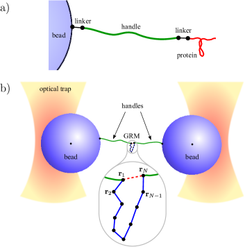
Figure S1: a) Schematic illustration (not to scale) of the covalent linkers which attach the handle to the bead on one end, and the handle to the protein on the other end. b) The Generalized Rouse Model (GRM) within the optical tweezer.

In some experimental setups, covalent linkers are attached on both ends of each handle, connecting the handle to the neighboring bead and protein, as schematically drawn in Fig. S1(a). The effect of linkers can be absorbed into the theory by modifying $\tilde{P}_{\text{h}}(k;F_{0})$. The simplest representation of a linker is a harmonic spring with stiffness $\kappa$ and natural length $\ell$. With one of these added at each end of the handle, Eq. (S15) becomes:

$$\tilde{\cal P}_{\text{h}}(k;F_{0})=\frac{Z_{\text{h}}(\beta F_{0}-ik)}{Z_{\text{h}}(\beta F_{0})}\frac{Z_{\text{link}}^{2}(\beta F_{0}-ik;\kappa,\ell)}{Z_{\text{link}}^{2}(\beta F_{0};\kappa,\ell)},$$ (S21)

where

$$\begin{split}Z_{\text{link}}(f;\kappa,\ell)&=\frac{1}{f}\sqrt{\frac{\pi}{2(\beta\kappa)^{3}}}e^{\frac{f(f-2\ell\beta\kappa)}{2\beta\kappa}}\Biggl{[}\ell\beta\kappa\,\text{erf}\left(\frac{f-\ell\beta\kappa}{\sqrt{2\beta\kappa}}\right)\\ &\qquad+e^{2f\ell}(f+\ell\beta\kappa)\left(\text{erf}\left(\frac{f+\ell\beta\kappa}{\sqrt{2\beta\kappa}}\right)+1\right)+f\text{erfc}\left(\frac{f-\ell\beta\kappa}{\sqrt{2\beta\kappa}}\right)-\ell\beta\kappa\Biggr{]}.\end{split}$$ (S22)

I.6 Numerical deconvolution to extract the protein distribution

The expressions given by Eq. (S9) and (S21) completely determine the Fourier-transformed point spread function $\tilde{\cal P}_{\text{bh}}(k;F_{0})$ at all $k$. Naively, one could use Eq. (S7) to write:

$$\tilde{\cal P}_{\text{p}}(k;F_{0})=\frac{\tilde{\cal P}_{\text{tot}}(k;F_{0})}{\tilde{\cal P}_{\text{bh}}(k;F_{0})}.$$ (S23)

Since $\tilde{\cal P}_{\text{tot}}(k;F_{0})$ is derivable from the experimental times series, this would immediately yield $\tilde{\cal P}_{\text{p}}(k;F_{0})$, and after inversion the ultimate goal, $\tilde{\cal P}_{\text{p}}(z_{\text{p}};F_{0})$. However, this direct deconvolution in Fourier space is numerically unstable Press07 , due to the effects of round-off noise and the denominator in the equation for $\tilde{\cal P}_{\text{p}}(k;F_{0})$ approaching zero at large $k$.

To work around this problem, we implement the deconvolution in real space, by solving the following integral equation for $\tilde{\cal P}_{\text{p}}$ (the real space version of Eq. (S7)):

$$\int dz_{\text{p}}\,\tilde{\cal P}_{\text{bh}}(z_{\text{tot}}-z_{\text{p}};F_{0})\tilde{\cal P}_{\text{p}}(z_{\text{p}};F_{0})=\tilde{\cal P}_{\text{tot}}(z_{\text{tot}};F_{0}).$$ (S24)

One way to approach Eq. (S24) is to approximate the integral as a matrix-vector product by discretizing the $z_{\text{tot}}$ and $z_{\text{p}}$ ranges. However, the convolution matrix corresponding to $\tilde{\cal P}_{\text{bh}}$ is generally ill-conditioned, so direct inversion to find a solution is unfeasible. Alternatively, to obtain robust, smooth results for the deconvolution, we can rewrite Eq. (S24) by representing the three quantities $\tilde{\cal P}_{\text{p}}$, $\tilde{\cal P}_{\text{bh}}$, and $\tilde{\cal P}_{\text{tot}}$ in terms of suitable fitting functions. Since these are all probability distributions, in practice we can approximate them to arbitrary precision as sums of Gaussians $g(z;\zeta,v)=(2\pi v)^{-1/2}\exp(-(z-\zeta)^{2}/(2v))$,

$$\tilde{\cal P}_{\alpha}(z_{\alpha};F_{0})=\sum_{i=1}^{N_{\alpha}}a^{\alpha}_{i}g(z_{\alpha};\zeta^{\alpha}_{i},v^{\alpha}_{i}),$$ (S25)

where $\alpha=\text{p}$, bh, or tot. The number of Gaussians needed for each distribution, $N_{\alpha}$, is chosen depending on the problem. The two sets of parameters $\{a^{\text{tot}}_{i},\xi^{\text{tot}}_{i},v^{\text{tot}}_{i}\}$ and $\{a^{\text{bh}}_{i},\xi^{\text{bh}}_{i},v^{\text{bh}}_{i}\}$ (which implicitly depend on $F_{0}$) are computed by fitting to the known functions $\tilde{\cal P}_{\text{tot}}$ and $\tilde{\cal P}_{\text{bh}}$. The goal of the procedure is then to use Eq. (S24) to solve for the parameter set $\{a^{\text{p}}_{i},\xi^{\text{p}}_{i},v^{\text{p}}_{i}\}$ describing the unknown function $\tilde{\cal P}_{\text{p}}$. For the cases discussed in the main text, choosing $N_{\alpha}=2-3$ was sufficient to find solutions $\tilde{\cal P}_{\text{p}}$ such that the left and right-hand sides of Eq. (S24) had a median deviation $\lesssim 1\%$ over all $z_{\text{tot}}$ where ${\cal P}_{\text{tot}}(z_{\text{tot}})\gtrsim 10^{-6}$.

The details of the solution procedure are as follows: we choose $N_{\text{p}}=N_{\text{tot}}$, so that Eq. (S24) can be approximated as a one-to-one convolution mapping each Gaussian in $\tilde{\cal P}_{\text{p}}$ into a corresponding Gaussian in $\tilde{\cal P}_{\text{tot}}$. For all $i=1,\ldots,N_{\text{tot}}$, Eq. (S24) describes the following relationships between the amplitudes, positions and variances of the Gaussians:

$$\begin{split}a^{\text{tot}}_{i}&\approx a^{\text{p}}_{i},\\ \xi^{\text{tot}}_{i}&\approx\sum_{j=1}^{N_{\text{bh}}}a^{\text{bh}}_{j}(\xi^{\text{bh}}_{j}+\xi^{\text{p}}_{i}),\\ v^{\text{tot}}_{i}&\approx\sum_{j=1}^{N_{\text{bh}}}a^{\text{bh}}_{j}(v^{\text{bh}}_{j}+v^{\text{p}}_{i}+(\xi^{\text{bh}}_{j}+\xi^{\text{p}}_{i})^{2}).\\ \end{split}$$ (S26)

The approximation is exact when the point-spread function $\tilde{\cal P}_{\text{bh}}$ is precisely a single Gaussian, but is generally valid whenever $\tilde{\cal P}_{\text{bh}}$ is close to Gaussian (as is the case for the bead-handle system, where the corrections introduced by choosing $N_{\text{bh}}>1$ are small). Eq. (S26) can be inverted to yield the desired parameter set $\{a^{\text{p}}_{i},\xi^{\text{p}}_{i},v^{\text{p}}_{i}\}$:

$$\begin{split}a^{\text{p}}_{i}&\approx a^{\text{tot}}_{i},\\ \xi^{\text{p}}_{i}&\approx\xi^{\text{tot}}_{i}-\sum_{j=1}^{N_{\text{bh}}}a^{\text{bh}}_{j}\xi^{\text{bh}}_{j},\\ v^{\text{p}}_{i}&\approx v^{\text{tot}}_{i}-\sum_{j=1}^{N_{\text{bh}}}a^{\text{bh}}_{j}\left[v^{\text{bh}}_{j}+\left(\xi^{\text{bh}}_{j}+\xi^{\text{tot}}_{i}-\sum_{k=1}^{N_{\text{bh}}}a^{\text{bh}}_{k}\xi^{\text{bh}}_{k}\right)^{2}\right],\\ \end{split}$$ (S27)

where we have used the fact that $\sum_{i}^{N_{\text{bh}}}a^{\text{bh}}_{i}=1$ due to normalization.

II Experimental verification of the model for the point-spread function

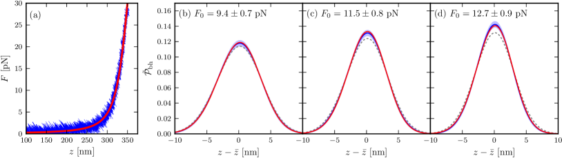
Figure S2: Experimental (blue solid curves) and theory (red solid curves) results for a system containing only dsDNA handles and beads. The apparatus parameters and theoretical best-fit values are described in Sec. II. The same set of best-fit parameters is used for all the theory curves. (a) Force $F$ vs. total extension $z$ from an experimental pulling trajectory, compared to the theoretical mean extension as a function of force; (b-d) Total bead-handle probability end-to-end distance distributions $\tilde{\cal P}_{\text{bh}}$ (blue solid curves) derived from three experimental runs at different constant trap separations, corresponding to mean forces of $9.4\pm 0.7$, $11.5\pm 0.8$, and $12.7\pm 0.9$ pN respectively. In each case the experimental data is corrected for noise/filtering effects using the FBS method (Sec. VI), and transformed into the constant force ensemble using Eq. [1] of the main text, with $F_{0}$ chosen to be equal to the mean force value in the trajectory. The distance scale is centered at $\bar{z}$, the mean extension. The light blue shaded region around each blue curve represents the standard error margin for every point in the distribution (68% confidence band). For comparison, the experimental results omitting the FBS corrections are shown as gray dashed lines.

In order to check that the theoretical model of the point-spread function $\tilde{\cal P}_{\text{bh}}$ derived in Secs. I.4-I.5 is an accurate description of the handle and bead response in experiments, we analyzed control experiments on a system with only dsDNA handles and beads. Bead radii are $R_{b}=500\pm 25$ nm, the trap strength is $k_{\text{trap}}=0.29\pm 0.02$ pN/nm, and the handle parameters are extracted from the theoretical best-fit described below. Four distinct experimental data sets are collected (Fig. S2): the first is from a pulling setup, where the trap separation is varied to give a trajectory of force $F$ vs. total extension $z$ (Fig. S2(a), blue curve); the other data sets are trajectories of extension $z$ as a function of time collected at three different constant trap separations. These three trajectories can be binned, and projected onto the constant force ensemble using the same method (Eq. (S5)) as described above for the full system, yielding probability distributions $\tilde{\cal P}_{\text{bh}}(z;F_{0})$ for the total end-to-end extension of the bead-handle system (Fig. S2(b-d), blue curves). The constant force value $F_{0}$ for each projection is chosen equal to the mean force in each of the three trajectories, namely $F_{0}=9.4\pm 0.7$, $11.5\pm 0.8$, and $12.7\pm 0.9$ pN.

The experimental data were collected at 100 kHz, with no additional time averaging beyond the electronic filtering intrinsic to the detection and recording apparatus. Prior to the projection onto the constant force ensemble, the FBS method (Sec. VI) was used to approximately correct the raw experimental data for distortions due to electronic filtering and noise. In the absence of these corrections, the $\tilde{\cal P}_{\text{bh}}(z;F_{0})$ from the raw data is given by the dashed curves in Fig. S2(b-d).

The standard error margin (68% confidence interval) for each point in the $\tilde{\cal P}_{\text{bh}}$ distribution is marked by a light blue band, reflecting uncertainties in apparatus and FBS parameters, as well as statistical error due to sampling. Details of the error estimation procedure are in Sec. VII. The median standard error in the $z$ range shown varies from $3-5\%$ between the three trajectories.

We use the theoretical model of Secs. I.4-I.5 to simultaneously fit all four experimental data sets with a single set of handle parameters, yielding best fit values: $L=173\pm 2$ nm, $l_{p}=11\pm 1$ nm, and $\gamma=520\pm 70$ pN. The theory has excellent agreement with all the experimental results, with median deviations in $\tilde{\cal P}_{\text{bh}}(z;F_{0})$ for the $z$ range shown in Fig. S2(b-d) varying from $1-3\%$ between the three trajectories, comparable to the standard error margins. The comparison between theory and experiments firmly establishes the remarkable accuracy of our theory in quantitatively describing the bead-handle system.

III Generalized Rouse Model (GRM)

III.1 Hamiltonian and exact probability distribution for the GRM

The GRM model Hyeon08 , illustrated schematically in Fig. S1(b), is a Gaussian chain with $N$ monomers, connected by $N-1$ harmonic springs with an average extension $a$. A conformation of the GRM is specified by the monomer positions $\mathbf{r}_{i}$, $i=1,\ldots,N$. To get behavior reminiscent of hairpin unzipping, an additional harmonic bond potential, $V(|\mathbf{r}_{N}-\mathbf{r}_{1}|)$, is added between the end-points $\mathbf{r}_{1}$ and $\mathbf{r}_{N}$; the force due to this potential is non-zero only if the end-point separation is within a cutoff distance, $c$. Under a constant external tension, $F_{0}\hat{\mathbf{z}}$, the GRM Hamiltonian is

$${\cal H}_{\text{GRM}}=\frac{3k_{B}T}{2a^{2}}\sum_{i=1}^{N-1}(\mathbf{r}_{i+1}-\mathbf{r}_{i})^{2}+V(|\mathbf{r}_{N}-\mathbf{r}_{1}|)-F_{0}\hat{\mathbf{z}}\cdot(\mathbf{r}_{N}-\mathbf{r}_{1}),$$ (S28)

where $V(r)=kr^{2}\Theta(c-r)+kc^{2}\Theta(r-c)$, and $\Theta$ is the unit step function. We choose parameters: $N=18$, $F_{0}=2.9$ $k_{B}T/$nm (11.9 pN), $a=1$ nm, $c=12$ nm, $k=0.09$ $k_{B}T/$nm² (0.37 pN/nm).

If we write the end-to-end vector $\mathbf{r}_{N}-\mathbf{r}_{1}$ in cylindrical coordinates as $(\rho,\phi,z)$, the exact probability distribution for this vector in equilibrium under constant force $F_{0}\hat{\mathbf{z}}$ is given by:

$$\tilde{\cal P}_{\text{GRM}}(\rho,\phi,z;F_{0})=A_{\text{GRM}}\exp\left(-\frac{3(\rho^{2}+z^{2})}{2a^{2}(N-1)}-\beta V(\sqrt{\rho^{2}+z^{2}})+\beta F_{0}z\right),$$ (S29)

where $A_{\text{GRM}}$ is a normalization constant. This distribution, projected onto the $(\rho,z)$ plane, is illustrated in the top panel of Fig. 2(a) in the main text. The peak at small $z$ corresponds to the “folded” hairpin state (F) with an intact end-point bond, while the peak at larger $z$ is the unfolded (U) state. Integrating $\tilde{\cal P}_{\text{GRM}}(\rho,\phi,z;F_{0})$ over $\rho$ and $\phi$ one obtains the marginal probability $\tilde{\cal P}_{\text{GRM}}(z;F_{0})$,

$$\begin{split}\tilde{\cal P}_{\text{GRM}}(z;F_{0})&=A^{\prime}_{\text{GRM}}e^{-\frac{3z^{2}}{2a^{2}(N-1)}+\beta F_{0}z}\\ \qquad&\cdot\begin{cases}e^{-\frac{c^{2}(3+2a^{2}\beta k(N-1))-3z^{2}}{2a^{2}(N-1)}}-\frac{3e^{-\beta kz^{2}}}{3+2a^{2}\beta k(N-1)}\left(e^{-(c^{2}-z^{2})\left(\beta k+\frac{3}{2a^{2}(N-1)}\right)}-1\right)&z\leq c\\ e^{-\beta kc^{2}}&z>c\end{cases},\end{split}$$ (S30)

with normalization constant $A^{\prime}_{\text{GRM}}$. $\tilde{\cal P}_{\text{GRM}}(z;F_{0})$ is plotted in the lower panel of Fig. 2(a).

III.2 Testing the GRM deconvolution at various forces and trap strengths

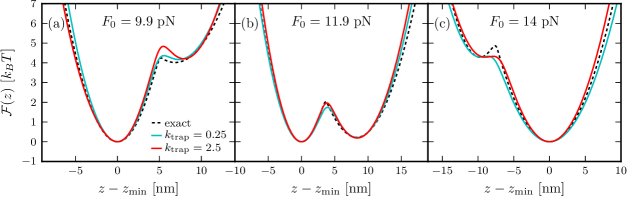
Figure S3: The GRM free energy $\tilde{F}_{\text{GRM}}$ after deconvolution for three different values of the force $F_{0}$: (a) 9.9 pN; (b) 11.9 pN; (c) 14 pN. In each case, results for two different trap strengths $k_{\text{trap}}=0.25$, $2.5$ pN/nm are shown as solid lines of different color. The exact analytical solutions are drawn as dashed lines. The $z$ scale is plotted relative to $z_{\text{min}}$, the location of the minimum in the free energy.

In Fig. 3(b) in the main text we showed that the deconvolution results for the GRM are robust when varying the handle parameters. In Fig. S3 we demonstrate that the same conclusion holds when either the force $F_{0}$ or the trap strength $k_{\text{trap}}$ are varied.

IV WHAM: combining trajectories from experimental runs at different trap separations

The weighted histogram analysis method Ferrenberg89 (WHAM) is a powerful tool in analyzing optical tweezer experiments. By combining trajectories generated at different trap separations $z_{\text{trap}}$ (resulting in different force scales $\bar{F}$), one can sample the full extent of the protein free energy landscape, and use WHAM to construct a single energy profile using all the trajectory data, as has been previously done in Ref. Shirts08 (and in a related, but different manner in Ref. Messieres11 .) In the context of our theory, WHAM modifies Step 1 of our procedure, allowing us to derive the equilibrium probability $\tilde{\cal P}_{\text{tot}}(z_{\text{tot}};F_{0})$ at constant force $F_{0}$ based on information from multiple experimental trajectories. Consider a set of $M$ experimental runs, where the $i$th trajectory consists of $n_{i}$ data points and has a trap separation $z^{(i)}_{\text{trap}}$. Except for $z^{(i)}_{\text{trap}}$, all other system parameters are kept the same between runs. For each run one can calculate the normalized histogram of total end-to-end distances $z_{\text{tot}}$, yielding a probability distribution ${\cal P}_{\text{tot}}^{(i)}(z_{\text{tot}})$. This distribution is related to ${\cal Q}_{\text{tot}}(z_{\text{tot}})$, the unbiased $z_{\text{tot}}$ probability in the absence of a trapping potential or external force, through Eq. (S4). Inverting that equation, we can write

$$\begin{split}{\cal Q}_{\text{tot}}(z_{\text{tot}})&\approx C_{i}^{-1}e^{\frac{1}{4}\beta k_{z}(z_{\text{trap}}^{(i)}-z_{\text{tot}})^{2}}{\cal P}_{\text{tot}}^{(i)}(z_{\text{tot}})\\ &\equiv e^{\beta(U_{i}(z_{\text{tot}})-F_{i})}{\cal P}_{\text{tot}}^{(i)}(z_{\text{tot}}),\end{split}$$ (S31)

where $C_{i}$ is a normalization constant, $U_{i}(z_{\text{tot}})=k_{z}(z_{\text{trap}}^{(i)}-z_{\text{tot}})^{2}/4$ and $F_{i}=\beta^{-1}\ln C_{i}$. In the case of one trajectory ($M=1$), Eq. (S31) is a way to estimate ${\cal Q}_{\text{tot}}(z_{\text{tot}})$, from which one can calculate $\tilde{\cal P}_{\text{tot}}(z_{\text{tot}};F_{0})=\exp(\beta F_{0}z_{\text{tot}}){\cal Q}_{\text{tot}}(z_{\text{tot}})$. This is just the standard Step 1 procedure described earlier.

When $M>1$, Eq. (S31) provides a different estimate of ${\cal Q}_{\text{tot}}(z_{\text{tot}})$ for each $i$, which ideally should be combined to give a single best approximation. The WHAM method resolves this problem, yielding a best estimate for ${\cal Q}_{\text{tot}}(z_{\text{tot}})$ of the form:

$${\cal Q}_{\text{tot}}(z_{\text{tot}})=A\frac{\sum_{i=1}^{M}n_{i}{\cal P}_{\text{tot}}^{(i)}(z_{\text{tot}})}{\sum_{j=1}^{M}n_{j}e^{-\beta(U_{j}(z_{\text{tot}})-F_{j})}},$$ (S32)

where $A$ is a normalization constant. The unknown parameters $\{F_{i}\}$ are given by:

$$F_{i}=-\frac{1}{\beta}\ln\left[\int dz_{\text{tot}}{\cal Q}_{\text{tot}}(z_{\text{tot}})e^{-\beta U_{i}(z_{\text{tot}})}\right].$$ (S33)

Eqs. (S32) and (S33) are a coupled system of equations for ${\cal Q}_{\text{tot}}(z_{\text{tot}})$ and $\{F_{i}\}$. We solve these by making an initial guess for the set $\{F_{i}\}$, substituting it into Eq. (S32) to find ${\cal Q}_{\text{tot}}(z_{\text{tot}})$, and using this estimate for ${\cal Q}_{\text{tot}}(z_{\text{tot}})$ in Eq. (S33) to find a new set of $\{F_{i}\}$. The process is iterated until we converge to a self-consistent solution to both equations. Once we have a best estimate of ${\cal Q}_{\text{tot}}(z_{\text{tot}})$, we can calculate $\tilde{\cal P}_{\text{tot}}(z_{\text{tot}};F_{0})$ as above, completing Step 1 of the construction.

V Leucine zipper simulations

V.1 SOP model for the LZ26 leucine zipper

The amino acid sequence for a single $\alpha$-helical strand of the LZ26 coiled coil is as follows (grouped into heptad repeats): MCQLEQK VEELLQK NYHLEQE VARLKQL VGELEQK VEELLQK NYHLEQE VARLKQL VGELEQK VEELLQK NYHLEQE VARLKQL VGEC. The sequence is the same as in Ref. Gebhardt10 , except that we have left out four residues at the beginning and three from the final heptad, for a total of 88 residues per strand. As in the experiment Gebhardt10 , the handles are attached at the cysteine in position b of the first heptad, and the cross-linking between strands is at the cysteine in position d of the last heptad. (For consistency when comparing simulations with or without the handles/traps, end-to-end distance for the protein is always measured between the two N-terminal cysteines.) Although the crystal structure is not available for LZ26, it is believed to be similar to three GCN4 leucine zipper domains (PDB ID code 2ZTA) OShea91 in series. Thus, we constructed a model for the native structure based on GCN4, connecting the leucine zipper segments in such a way that the distances between neighboring $C_{\alpha}$ positions and angles of superhelical coiling formed a continuous pattern as one moves along LZ26.

Going from N- to C-terminus on one strand and returning C- to N-terminus on the other, let us label the residues $i=1,\ldots,N_{\text{res}}$, where $N_{\text{res}}=176$, where $1\leq i\leq 88$ corresponds to one strand, and $88<i\leq 176$ corresponds to the other. Every non-neighboring pair of residues, $(i,j)$ where $|i-j|>1$, is assigned to one of three sets: ${\cal S}$ (secondary structure pairs), ${\cal T}$ (tertiary structure pairs), and ${\cal R}$ (remainder). The set ${\cal S}$ consists of all pairs where $|i-j|=4$ and $i$, $j$ share the same strand, representing residues interacting through $\alpha$-helical hydrogen bonding. The set ${\cal T}$ consists of all pairs where $i$, $j$ are on different strands, and the distance between the two residues in the native structure, $r^{0}_{i,j}$, is below a cutoff: $r^{0}_{i,j}<R_{c}=0.8$ nm. These pairs are involved in tertiary interactions between the two $\alpha$-helical coils. All other non-neighboring pairs that do not satisfy the criteria for ${\cal S}$ or ${\cal T}$ fall into the set ${\cal R}$, and only interact via repulsive Lennard-Jones potentials.

The variant SOP Hamiltonian for LZ26 has the form:

$$\begin{split}{\cal H}_{\text{SOP}}=&\frac{k_{\text{bond}}}{2}\sum_{i=1}^{N_{\text{res}}-1}(r_{i,i+1}-r_{i,i+1}^{0})^{2}+\frac{k_{\text{ang}}}{2}\sum_{i=1}^{N_{\text{res}}-2}\left[1-\cos(\theta_{i,i+1,i+2}-\theta_{0})\right]\Delta_{i,i+1,i+2}\\ &-\sum_{(i,j)\in{\cal S}}\epsilon_{\text{hb}}\left[1+k^{\text{hb}}_{\text{bond}}(r_{i,j}-r_{i,j}^{0})^{2}+k^{\text{hb}}_{\text{ang}}\left((\theta_{i,j,j-1}-\theta_{i,j,j-1}^{0})^{2}+(\theta_{i+1,i,j}-\theta_{i+1,i,j}^{0})^{2}\right.\right.\\ &\qquad\qquad\qquad\left.\left.+(\phi_{i+1,i,j,j-1}-\phi_{i+1,i,j,j-1}^{0})^{2}\right)\right]^{-1}\\ &+\sum_{(i,j)\in{\cal T}}\chi|\epsilon_{\text{BT}}(i,j)-\epsilon_{s}|V_{\text{LJ}}\left(\frac{r^{0}_{i,j}}{r_{i,j}}\right)+\sum_{(i,j)\in{\cal R}}\epsilon_{\text{rep}}\left(\frac{\sigma}{r_{i,j}}\right)^{6}.\end{split}$$ (S34)

The first term is the nearest-neighbor bond potential, where $r_{i,j}$ is the distance between residues $i$ and $j$, and the spring constant $k_{\text{bond}}=200$ kcal/mol$\cdot$nm². The second term is the bond angle potential, with the spring constant $k_{\text{ang}}=2$ kcal/mol. The angle between the bonds $(j,i)$ and $(j,k)$ is $\theta_{i,j,k}$, and the equilibrium value $\theta_{0}=0.583\pi\>\text{rad}=105^{\circ}$, a typical bond angle in protein structures Klimov98 . The factor $\Delta_{i,j,k}=1$ if $i$, $j$, $k$ are all on the same strand, 0 otherwise. The relative softness of the bond angle potential, together with the form of the secondary structure interactions detailed below, ensure that the two strands in the unfolded LZ26 (with all inter-strand tertiary contacts broken) have a persistence length of $\sim 0.7$ nm, consistent with experimental measurements Gebhardt10 .

The third term in Eq. (S34) accounts for the effects of hydrogen bonding along the $\alpha$-helical backbone, and is based on a similar form developed for RNA Denesyuk11 . We mimic the directionality-dependence of hydrogen bonds by making the bond energy depend not only on the distance $r_{i,j}$, but also on bond and dihedral angles defined by the four residues $i+1$, $i$, $j$, and $j-1$, with $|i-j|=4$. For each $(i,j)$ there are two bond angles, $\theta_{i,j,j-1}$ and $\theta_{i+1,i,j}$, and one dihedral angle, $\phi_{i+1,i,j,j-1}$. The equilibrium values of the angles, denoted by a superscript 0, are calculated from the corresponding quantities in the native structure. Only when the distance, bond angles, and dihedral angles are all simultaneously equal to the equilibrium values does the hydrogen bond potential reach its energy minimum $-\epsilon_{\text{hb}}$, where $\epsilon_{\text{hb}}>0$. Thus, the minimum is reached only when the entire $(i,i+4)$ strand segment adopts a structure resembling a single $\alpha$-helical turn. The $\alpha$-helical propensity of an $(i,i+4)$ segment is determined by the energy scale $\epsilon_{\text{hb}}$ and the sensitivity parameters $k_{\text{bond}}^{\text{hb}}$, $k_{\text{ang}}^{\text{hb}}$. Larger values for the sensitivity parameters increase the brittleness of the $\alpha$-helix, making it more likely to be destablized due to thermal fluctuations. To calibrate the parameters, we define a helix function $H(i,j)$ for any $(i,j)\in{\cal S}$,

$$H(i,j)=\sqrt{\left(\frac{r_{i,j}}{r_{i,j}^{0}}-1\right)^{2}+\left(\frac{\theta_{i,j,j-1}}{\theta_{i,j,j-1}^{0}}-1\right)^{2}+\left(\frac{\theta_{i+1,i,j}}{\theta_{i+1,i,j}^{0}}-1\right)^{2}+\left(\frac{\phi_{i+1,i,j,j-1}}{\phi_{i+1,i,j,j-1}^{0}}-1\right)^{2}},$$ (S35)

reflecting the RMS deviation of the bond distances and angles from their equilibrium values. We use $H(i,j)$ as a measure of helix content, by counting the fraction of pairs in ${\cal S}$ where $H(i,j)$ is less than a cutoff $H_{\text{c}}=0.5$. It is known from thermal denaturation experiments on GCN4 Holtzer01 that the individual $\alpha$ helices upon unzipping are unstable, with $\approx 17\%$ helical content. In contrast, the tertiary contacts in the coiled-coil structure stabilize helix formation, resulting in a much higher helical content of $\approx 81\%$. We expect qualitatively similar behavior in LZ26 in the case of force denaturation, and thus tune the sensitivity parameters to yield a large difference in the helix content between the unfolded and folded states. The parameter values are set at $\epsilon_{\text{hb}}=3.85$ kcal/mol, $k^{\text{hb}}_{\text{bond}}=10$ nm^-2, $k^{\text{hb}}_{\text{ang}}=40$ rad^-2. For these values we find a helix content of 3% and 82% respectively for the unfolded and folded states of LZ26 under a constant force of $F_{0}=12.3$ pN.

The fourth term in Eq. (S34) describes tertiary interactions between the two strands of LZ26, $(i,j)\in{\cal T}$. These have a residue-dependent energy $\chi|\epsilon_{\text{BT}}(i,j)-\epsilon_{s}|$. Here $\chi$ is an overall prefactor, $\epsilon_{\text{BT}}(i,j)$ is the Betancourt-Thirumalai (BT) contact energy for residues $i$ and $j$ Betancourt99 , and $\epsilon_{s}$ shifts the zero of the energy scale Liu11 . To get a leucine zipper that unfolds at the experimental force scale of $\sim 12$ pN, we choose $\chi=2.25$ and energy shift $\epsilon_{s}=0.7$ $k_{B}T$. The tertiary interactions use a modified Lennard-Jones potential of the form:

$$V_{\text{LJ}}(x)=\begin{cases}x^{6}-\frac{3}{2}x^{4}-\frac{1}{2}&x\leq 1\\ x^{12}-2x^{6}&x>1\end{cases}.$$ (S36)

This has the standard 12-6 form at large distances, but a softer short-range repulsive core, increasing with the inverse 6th rather than 12th power. The choice of the softer potential is made to allow for a longer simulation time step, while not having a significant impact on the large-scale dynamics of the system Hyeon06 .

The final term in Eq. (S34) describes purely repulsive interactions among the remaining non-neighboring pairs, $(i,j)\in{\cal R}$, with energy factor $\epsilon_{\text{rep}}=1$ kcal/mol and range $\sigma=0.38$ nm. We use the inverse 6th power in the repulsive potential for the same reasons as above.

V.2 Semiflexible bead-spring model for the DNA handles

Each double-stranded DNA handle is modeled as a chain of $N_{\text{h}}$ beads of radius $a=1$ nm, corresponding to a contour length $L=2aN_{\text{h}}$. The handle Hamiltonian is:

$$\begin{split}{\cal H}_{\text{h}}=\frac{k_{\text{bond}}}{2}\sum_{i=1}^{N_{\text{h}}-1}(r_{i,i+1}-2a)^{2}+\frac{l_{p}k_{B}T}{2a}\sum_{i=1}^{N_{\text{h}}-2}\left[1-\cos(\theta_{i,i+1,i+2})\right]\end{split}$$ (S37)

where $r_{i,i+1}$ are the distances between neighboring beads, $k_{\text{bond}}=200$ kcal/mol$\cdot$nm², $l_{p}$ is the persistence length, and $\theta_{i,i+1,i+2}$ are angles between consecutive bonds. The two terms are stretching and bending energies respectively. The handle elastic modulus $\gamma=2ak_{\text{bond}}=2780$ pN. For the persistence length we consider, $l_{p}=20$ nm, at the applied tension due to the traps, the handles (and unfolded portions of the protein) are almost fully extended, and there is negligible probability of the chain overlapping itself or protein residues in the vicinity of the handle attachment point. Hence, there is no need to include excluded volume interactions for the handles. The covalent linkers that attach the handles either to the cysteine residue at the protein N-terminus or a point on the bead surface are modeled as simple harmonic springs with strength $\kappa=k_{\text{bond}}$ and length $\ell=1.5$ nm.

V.3 Simulation time scales

Let $\mu_{0}=1/6\pi\eta a$ be the mobility of a sphere of radius $a=1$ nm, where $\eta=0.89$ mPa$\cdot$s is the viscosity of water at $T=298$ K. This will be the mobility of our DNA handle beads, while for the large polystyrene beads the corresponding mobility is $\mu_{\text{b}}=\mu_{0}a/R_{b}$. The rotational diffusion of the polystyrene bead is characterized by a mobility $\mu_{\text{b}}^{r}=3\mu_{0}a/4R_{b}^{3}$. For the protein residues we choose a mobility $\mu_{\text{res}}=3.36\mu_{0}$, corresponding to an effective hydrodynamic radius of $0.30$ nm. The characteristic Brownian dynamics time scale associated with $\mu_{0}$ is $\tau_{0}=a^{2}/\mu_{0}k_{B}T=4$ ns. To avoid numerical errors, our simulation time step $\tau$ should be a small fraction of $\tau_{0}$, and we obtained reliable results using $\tau=5\times 10^{-6}\tau_{0}=0.02$ ps. For LZ26 both with and without handles/beads, we ran $\approx 260$ long trajectories at various force conditions (or trap separations), totaling to $\approx 10^{12}$ simulation time steps, or $20$ ms, with data collection every $10^{4}$ steps. (In the case of the simulations involving the GRM hairpin instead of the protein, the time step $\tau=3\times 10^{-4}\tau_{0}=1.2$ ps, and the total trajectory data for each GRM parameter set corresponded to $160-180$ ms.)

VI Finite bandwidth scaling (FBS): correcting for the effects of electronic filtering, time averaging, and noise

Before the data from optical tweezer experiments can be used to reconstruct the intrinsic biomolecule free energy landscape, one must consider the inevitable distortions due to noise, the electronic systems involved in data recording, and any additional filtering done as part of the collection protocol. We have developed a method, finite bandwidth scaling (FBS), to correct for these distortions. In the following we first derive the basic FBS scaling relations, and then verify them using both simulation and experimental data sets.

VI.1 FBS theory

Understanding how the time series of bead positions is distorted as part of the measurement process requires a detailed spectral analysis of all components in the dual optical tweezer apparatus. The spectral properties of the experimental system used to collect the data in our work have been extensively characterized by von Hansen et. al. vonHansen12 , allowing us to develop a simplified theory which approximates the most important sources of distortion. Our theory fits all the experimental data sets under consideration, but it can be easily modified to include additional complications that we ignore (for example crosstalk between the two laser traps) as well as the details of other experimental setups.

Let $z^{\text{raw}}_{\text{tot}}(t)$ be the trajectory of bead-bead separations along the $\hat{\mathbf{z}}$-axis recorded during the experiment. This raw data set is based on the signal from the silicon photodiode devices that measure the deflection of the lasers due to bead displacements. This output is then processed and amplified by the electronic system used in the recording apparatus. If $z_{\text{tot}}(t)$ is the actual trajectory of bead displacements, inaccessible to the experimentalist, the recorded output $z^{\text{raw}}_{\text{tot}}(t)$ is related to $z_{\text{tot}}(t)$ as:

$$z^{\text{raw}}_{\text{tot}}(t)=\int_{-\infty}^{t}f(t-t^{\prime})(z_{\text{tot}}(t^{\prime})+\eta(t^{\prime})).$$ (S38)

The deviation of $z^{\text{raw}}_{\text{tot}}(t)$ from $z_{\text{tot}}(t)$ stems from two main effects: (i) an additive noise component $\eta(t)$, which includes environmental noise like vibrations of the optical elements in the apparatus and electronic noise in the detectors vonHansen12 . For simplicity, we model the noise as Gaussian white noise with zero mean and variance equal to $\nu$: $\langle\eta(t)\rangle=0$, $\langle\eta(t)\eta(t^{\prime})\rangle=\nu\delta(t-t^{\prime})$, and $\langle\eta(t)z_{\text{tot}}(t^{\prime})\rangle=0$, where $\langle\;\rangle$ denotes an equilibrium ensemble average; (ii) convolution with a kernel function $f(t)$, which reflects the filtering properties of the photodiodes and electronics. Any additional time averaging or filtering carried out by the experimentalist on the recorded data series will be considered explicitly later on, and is not included in $f(t)$. The analysis of Ref. vonHansen12 yielded the following form for the filter kernel in the frequency domain,

$$f(\omega)=\left[\lambda+\frac{1-\lambda}{1-i\omega\tau_{pf}}\right]\frac{1}{B_{8}(i\omega\tau_{bf})},$$ (S39)

where for our LOT setup $\lambda=0.6\pm 0.05$, $\tau_{pf}=6\pm 1$ $\mu$s, $\tau_{bf}=5$ $\mu$s, and $B_{8}(x)$ is the 8th order Butterworth polynomial. The term in the square brackets above originates in a physical phenomenon known as “parasitic filtering” Peterman03 ; Berg06 , arising from the transparency of the silicon in the photodiode to the laser light with wavelength 1064 nm used in the experiment: a fraction $1-\lambda$ of the photocurrent from the detector is produced with a lag time $\tau_{pf}$ relative to the photon signal. The second term in Eq. (S39), involving the Butterworth polynomial, is due to the subsequent electronic amplification of the signal from the detector, which acts like a Butterworth lowpass filter with characteristic timescale $\tau_{bf}$, such that at the frequency $\omega=\tau_{bf}^{-1}$ the signal amplitude is attenuated by 3 dB. Since the form of Eq. (S39) is too complicated for use in our analytical theory, we will approximate $f(t)$ as a generic first-order low-pass filter, exploiting the fact that both the parasitic and electronic terms act to attenuate high-frequency portions of the signal,

$$f(\omega)\approx\frac{1}{1-i\omega\tau_{f}},$$ (S40)

where $\tau_{f}=7$ $\mu$s. This effective filtering timescale $\tau_{f}$ is derived by demanding that Eq. (S40) exhibit the same degree of attenuation at $\omega=\tau_{bf}^{-1}$ as Eq. (S39).

Though these distortions are expressed in the frequency domain, they have observable consequences for the equilibrium probability distribution of bead-bead separations. As an example, consider the raw autocorrelation function $C_{\text{raw}}(t)=\langle(z^{\text{raw}}_{\text{tot}}(t)-\bar{z}^{\text{raw}}_{\text{tot}})(z^{\text{raw}}_{\text{tot}}(0)-\bar{z}^{\text{raw}}_{\text{tot}})\rangle$, where $\bar{z}^{\text{raw}}_{\text{tot}}$ is the mean recorded bead-bead separation. The variance of the raw probability distribution ${\cal P}^{\text{raw}}_{\text{tot}}(z^{\text{raw}}_{\text{tot}})$ is equal to $C_{\text{raw}}(0)$. From Eqs. (S38) and (S40), the raw autocorrelation is related to the true one, $C(t)=\langle(z_{\text{tot}}(t)-\bar{z}_{\text{tot}})(z_{\text{tot}}(0)-\bar{z}_{\text{tot}})\rangle$, by:

$$C_{\text{raw}}(t)=\frac{\nu}{2\tau_{f}}e^{-t/\tau_{f}}+\int_{-\infty}^{\infty}dt^{\prime}\,\frac{e^{-|t-t^{\prime}|/\tau_{f}}}{2\tau_{f}}C(t^{\prime}).$$ (S41)

The first term in Eq. (S41), due to noise, tends to increase the variance $C_{\text{raw}}(0)$ relative to $C(0)$. The second term, due to filtering, is always less than $C(0)$, since it is an average over $C(t^{\prime})$, and $C(t^{\prime}\neq 0)<C(0)$. Noise broadens the measured distribution, and filtering narrows it. However without knowing the amplitude of the noise $\nu$, it is unclear whether the filtering due to the detectors and electronics under- or over-compensates for the noise, and how far ${\cal P}^{\text{raw}}_{\text{tot}}(z^{\text{raw}}_{\text{tot}})$ deviates from the true distribution ${\cal P}_{\text{tot}}(z_{\text{tot}})$. Thus, we need a way to estimate $\nu$.

The situation is even more complicated since the experimentalist may choose to apply additional filtering on the recorded data, for example as a way of manually removing noise and unwanted high frequency components of the signal (since the dynamics of interest typically occur at frequencies much lower than imposed filter cutoff). For the GCN4 leucine zipper, the data sets recorded at 100 kHz (corresponding to a sampling time step $\tau_{s}=10$ $\mu$s) were subsequently filtered in real time during collection by averaging every 5 consecutive time steps together. Such averaging acts like a low-pass filter, and so has narrowing effects on the equilibrium probability distribution qualitatively similar to the filtering described above. Some type of additional filtering of this kind is a common experimental practice (see Refs. Gao11 ,Yu12 , and Ritchie12 for recent examples, involving either an averaging or 8 pole Bessel filter). It turns out, however, that we can take advantage of the filtering protocol: by varying the degree of filtering we will use it to approximately extrapolate features of the true probability distribution.

Let us concentrate on the simple case of filtering the recorded data by averaging every $n$ consecutive points into a single value. If the collection time step is $\tau_{s}$, the original raw data is represented by the recorded time series $\{z^{\text{raw}}_{\text{tot}}(t_{j})\}$, where $t_{j}\equiv j\tau_{s}$ for $j=1,2,3,\ldots$. The averaged data is a time series $\{z^{\text{raw,$n$}}_{\text{tot}}(t_{nj})\}$, where $z^{\text{raw,$n$}}_{\text{tot}}(t_{nj})=n^{-1}\sum_{i=nj-n+1}^{i=nj}z^{\text{raw}}_{\text{tot}}(t_{i})$. For the averaged time series we will focus on two quantities, both related directly to its autocorrelation $C_{\text{raw,$n$}}(t)$: the variance $\langle(z^{\text{raw,$n$}}_{\text{tot}}-\bar{z}^{\text{raw,$n$}}_{\text{tot}})^{2}\rangle=C_{\text{raw,$n$}}(0)$, and the mean-squared displacement (MSD) between consecutive points, $\langle(z^{\text{raw,$n$}}_{\text{tot}}(n\tau_{s})-z^{\text{raw,$n$}}_{\text{tot}}(0))^{2}\rangle=2(C_{\text{raw,$n$}}(0)-C_{\text{raw,$n$}}(n\tau_{s}))\equiv\Delta_{\text{raw,$n$}}(n\tau_{s})$. In a more complicated fashion, these two quantities can also be expressed in terms of the original autocorrelation $C_{\text{raw}}(t)=C_{\text{raw,1}}(t)$ before averaging:

$$\begin{split}C_{\text{raw,$n$}}(0)&=\frac{1}{n}C_{\text{raw}}(0)+\frac{2}{n^{2}}\sum_{j=1}^{n-1}(n-j)C_{\text{raw}}(j\tau_{s}),\\ \Delta_{\text{raw,$n$}}(n\tau_{s})&=\frac{2}{n}C_{\text{raw}}(0)+\frac{2}{n^{2}}\sum_{j=1}^{n}(2n-3j)C_{\text{raw}}(j\tau_{s})-\frac{2}{n^{2}}\sum_{j=1}^{n-1}(n-j)C_{\text{raw}}((n+j)\tau_{s}).\end{split}$$ (S42)

We know that $C_{\text{raw}}(t)$ is related to the unknown true correlation $C(t)$ through Eq. (S41), so we can complete the theoretical description by specifying a form for $C(t)$. A generic correlation function can be expanded as a sum of exponentials, $C(t)=\sum_{i=1}^{\infty}A_{i}\exp(-t/\tau_{i})$, with relaxation times $\tau_{1}<\tau_{2}<\cdots$. We will be interested in correlations on the shortest accessible time-scales, $t\sim{\cal O}(\tau_{s})$, so we plug the expression for $C(t)$ into Eq. (S41) and expand for small $t$, keeping the contribution from the $\tau_{1}$ exponential and lowest order corrections from the $\tau_{i>1}$ terms:

$$\begin{split}C_{\text{raw}}(t)&=\frac{\nu}{2\tau_{f}}e^{-t/\tau_{f}}+\sum_{i=1}^{\infty}\frac{A_{i}\tau_{i}}{\tau_{i}^{2}-\tau_{f}^{2}}\left(\tau_{i}e^{-t/\tau_{i}}-\tau_{f}e^{-t/\tau_{f}}\right)\\ &\approx\frac{\nu}{2\tau_{f}}e^{-t/\tau_{f}}+\frac{A_{1}\tau_{i}}{\tau_{1}^{2}-\tau_{f}^{2}}\left(\tau_{1}e^{-t/\tau_{1}}-\tau_{f}e^{-t/\tau_{f}}\right)+A_{c}-B_{c}(t+t_{f}e^{-t/\tau_{f}}),\end{split}$$ (S43)

where $A_{c}=\sum_{i=2}^{\infty}A_{i}$, $B_{c}=A_{2}/\tau_{2}$. If necessary, the expansion can be extended to higher orders, but the above form was sufficient to fit all the simulation and experimental cases which we analyze below.

Eqs. (S42)-(S43) completely define the variance $C_{\text{raw,$n$}}(0)$ and MSD $\Delta_{\text{raw,$n$}}(n\tau_{s})$ in terms of five unknown parameters: $\nu$, $A_{1}$, $\tau_{1}$, $A_{c}$, and $B_{c}$. By averaging the recorded time series $\{z^{\text{raw}}_{\text{tot}}(t_{j})\}$ for different values of $n$ (varying the effective filter bandwidth), we construct curves of $C_{\text{raw,$n$}}(0)$ and MSD $\Delta_{\text{raw,$n$}}(n\tau_{s})$ as a function of $n$. Fitting these curves to Eqs. (S42)-(S43), we can then extract the unknown parameters. This allows us to estimate the true variance of the probability distribution,

$$C(0)=A_{1}+A_{c}.$$ (S44)

Since we are using properties of time series at different effective bandwidths to gain information about the true, “infinite” bandwidth limit, we call our method finite bandwidth scaling (FBS). The analogy is to finite size scaling Ferdinand69 , where thermodynamic properties of systems on finite lattices are extrapolated to the infinite lattice limit. One of the nice features of FBS is that the scaling analysis can be carried out even when we can only calculate $C_{\text{raw,$n$}}(0)$ and $\Delta_{\text{raw,$n$}}(n\tau_{s})$ for a subset of $n$ values. For example, in the leucine zipper case below, the available time series corresponds to $n=5$, since the data was time averaged during collection. From the $n=5$ data we can construct trajectories for $n=10,15,20,\ldots$. This subset is sufficient for the FBS extrapolation.

Once we know $C(0)$, how can we use it to approximately reconstruct the true distribution ${\cal P}_{\text{tot}}(z_{\text{tot}})$? Keep in mind that the variance $C(0)=\langle z_{\text{tot}}^{2}\rangle-\langle z_{\text{tot}}\rangle^{2}=\int dz\,(z-\langle z_{\text{tot}}\rangle)^{2}{\cal P}_{\text{tot}}(z)$. The simplest estimate for ${\cal P}_{\text{tot}}(z_{\text{tot}})$ is to start with the measured, averaged distribution ${\cal P}^{\text{raw,$n$}}_{\text{tot}}$ for some $n$, and deform it in one of two ways, changing its variance by an amount $\delta_{C}=|C(0)-C_{\text{raw,$n$}}(0)|$: (i) If $C_{\text{raw,$n$}}(0)<C(0)$, we carry out a convolution with a normalized Gaussian of variance $\delta_{C}$,

$${\cal P}_{\text{tot}}(z_{\text{tot}})\approx\int_{-\infty}^{\infty}dz\,{\cal P}^{\text{raw,$n$}}_{\text{tot}}(z_{\text{tot}}-z)\frac{e^{-z^{2}/2\delta_{c}}}{\sqrt{2\pi\delta_{C}}}.$$ (S45)

(ii) If $C_{\text{raw,$n$}}(0)>C(0)$, we do a deconvolution instead, solving

$${\cal P}^{\text{raw,$n$}}_{\text{tot}}(z_{\text{tot}})\approx\int_{-\infty}^{\infty}dz\,{\cal P}_{\text{tot}}(z_{\text{tot}}-z)\frac{e^{-z^{2}/2\delta_{c}}}{\sqrt{2\pi\delta_{C}}}$$ (S46)

for ${\cal P}_{\text{tot}}$. The latter can be carried out using the numerical deconvolution technique described in Sec. I.6. After the deformation, the estimated ${\cal P}_{\text{tot}}$ will by construction have the correct variance $C(0)$. We should recover roughly the same ${\cal P}_{\text{tot}}$ starting from ${\cal P}^{\text{raw,$n$}}_{\text{tot}}$ for any $n$ in the range where the FBS scaling is valid, as we will demonstrate in the examples below. In systems with multiple states, where there is more than one peak in the measured distribution, it is more accurate to carry out the FBS analysis separately on each state, and apply the corresponding specific deformation for each peak. This can be done with the aid of hidden Markov model Rabiner89 partitioning of the time series, as described in the next section for the case of the GRM and leucine zipper.

The FBS method has several limitations: (i) using a Gaussian to deform ${\cal P}^{\text{raw,$n$}}_{\text{tot}}$ into ${\cal P}_{\text{tot}}$ is an assumption, since all we strictly know about the actual point-spread function is the variance $\delta_{C}$. The smaller the variance, the more valid the assumption, since the potential non-Gaussian contributions to the point-spread function become less significant. We can also test the assumption from our measured data, by checking whether the ${\cal P}^{\text{raw,$n$}}_{\text{tot}}$ for various $n$ can be mapped to each other by Gaussian deformations. For all the systems analyzed in our work this is indeed the case. (ii) Gaussian deformations map individual peaks into slightly broader or narrower peaks, but do not produce new peaks. Hence, if there is a state with a very short lifetime that is smeared out by the filtering (either the parasitic, electronic, or additional filtering), yielding no distinct peak in ${\cal P}^{\text{raw,$n$}}_{\text{tot}}$, the FBS method will not be able to reconstruct its properties. Whether or not the experimentalist chooses to do additional averaging, the intrinsic time resolution $\tau_{f}$ of the apparatus puts fundamental constraints on what we can learn from the measured time series. Transitions occurring on timescales faster than $\tau_{f}$ will be lost to us. (iii) In a similar way, the characteristic relaxation times of the trapped beads also impose limits. To illustrate this, take two protein states $S_{1}$ and $S_{2}$, which have a small difference in their mean end-to-end distance along the force direction, and assume $S_{1}$ is only accessible from $S_{2}$. If the mean lifetime of $S_{1}$ is much smaller than $S_{2}$, such that it is shorter than the bead relaxation time, transitions like $S_{2}\to S_{1}\to S_{2}$ will correspond to only negligible excursions in the measured trajectory of bead displacements, since the beads do not have enough time to relax to the equilibrium position associated with $S_{1}$ before the protein returns to $S_{2}$. If the mean-squared distance of the excursions is smaller than the noise amplitude in the recorded time series, the existence of state $S_{1}$ will be hidden from the experimentalist, regardless of the apparatus filtering timescale $\tau_{f}$. In summary, the distribution produced by FBS is an approximation to the truth: the method can correct distortions produced by noise and filtering, but it only works for states in the energy landscape which leave some signature of themselves in the measured time series.

Table S2: Parameters used in the FBS analysis of simulation and experimental systems

	$\tau_{s}$	$\tau_{f}$	$\nu$	$A_{1}$	$\tau_{1}$	$A_{c}$	$B_{c}$
	[$\mu$s]	[$\mu$s]	[nm${}^{2}\mu$s]	[nm2]	[$\mu$s]	[nm2]	[nm2/$\mu$s]
Simulation: GRM
State $N$	0.024	0	0	$2.2\pm 1.2$	$3.2\pm 1.0$	$3.1\pm 1.2$	$0.24\pm 0.15$
State $U$	0.024	0	0	$1.6\pm 0.2$	$2.1\pm 0.2$	$2.6\pm 0.2$	$0.22\pm 0.04$
Experiment: dsDNA handles (no protein)
$F_{0}=9.4$ pN	10	7	$31.8\pm 1.5$	$5.0\pm 0.2$	$14.7\pm 1.8$	$3.2\pm 0.2$	$0.0077\pm 0.0020$
$F_{0}=11.5$ pN	10	7	$31.8\pm 1.5$	$4.0\pm 0.2$	$12.6\pm 1.4$	$3.0\pm 0.1$	$0.0079\pm 0.0012$
$F_{0}=12.7$ pN	10	7	$31.8\pm 1.5$	$3.3\pm 0.2$	$11.5\pm 1.2$	$2.9\pm 0.1$	$0.0076\pm 0.0008$
Experiment: GCN4 leucine zipper (trajectory 1)
State I1	10	7	$31.8\pm 1.5$	$3.9\pm 0.2$	$28.1\pm 5.0$	$3.5\pm 0.2$	$0.0066\pm 0.0010$
State I2	10	7	$31.8\pm 1.5$	$8.6\pm 0.6$	$41.9\pm 8.0$	$4.2\pm 0.8$	$0.0069\pm 0.0036$
State U	10	7	$31.8\pm 1.5$	$7.6\pm 0.1$	$23.7\pm 1.7$	$3.2\pm 0.1$	$0.0065\pm 0.0007$
Experiment: GCN4 leucine zipper (trajectory 2)
State I1	10	7	$31.8\pm 1.5$	$4.1\pm 0.1$	$28.1\pm 3.5$	$3.5\pm 0.2$	$0.0069\pm 0.0008$
State I2	10	7	$31.8\pm 1.5$	$8.3\pm 1.0$	$41.3\pm 12.0$	$5.3\pm 1.3$	$0.0074\pm 0.0053$
State U	10	7	$31.8\pm 1.5$	$8.1\pm 0.2$	$23.6\pm 2.2$	$3.2\pm 0.2$	$0.0066\pm 0.0009$

VI.2 Testing FBS on simulation and experimental data

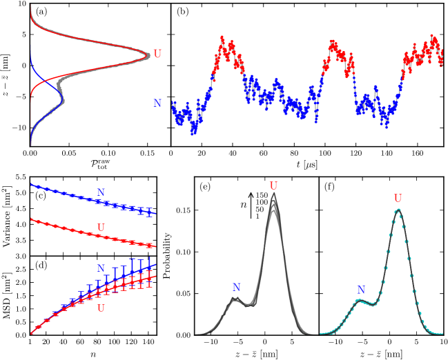
Figure S4: FBS analysis of a GRM Brownian dynamics simulation ($z_{\text{trap}}=1298$ nm; all other parameters as in Table S1). (a) The probability distribution of the bead-bead separation from the raw simulation data, ${\cal P}^{\text{raw}}_{\text{tot}}$ (gray), and the decomposition into individual Gaussian peaks corresponding to the N (blue) and U (red) states. Distances are measured with respect to $\bar{z}$, the mean bead-bead separation. (b) A sample time series fragment from the simulation, with the individual data points colored according to their assignment to the N (blue) and U (red) states by hidden Markov model analysis. (c) For the raw time series filtered by averaging together every $n$ data points, the variance $C_{\text{raw,$n$}}(0)$ as a function of $n$. The time series corresponding to each state, N and U, is analyzed separately, and plotted as blue and red points respectively, with bars denoting standard error due to finite sampling. The solid curves are the FBS theoretical fits to $C_{\text{raw,$n$}}(0)$ [Eq. (S42)]. Best-fit FBS parameters are listed in Table S2. (d) Analogous to (c), except showing the MSD function $\Delta_{\text{raw,$n$}}(n\tau_{s})$ for consecutive pairs of points in the averaged time series. (e) The raw distributions ${\cal P}^{\text{raw,$n$}}_{\text{tot}}$ for the averaged time series at $n=1$, 50, 100, 150. (f) Solid curves: the distribution ${\cal P}_{\text{tot}}$ estimated by applying the appropriate FBS correction to the raw distributions in (e). There are four curves, but due to overlapping they appear as one. Points: the raw distribution ${\cal P}^{\text{raw,$n$}}_{\text{tot}}$ for $n=1$ (no averaging), which for the GRM case is the true distribution, since there are no noise or apparatus filtering effects in the simulation.

As a first test of the FBS theory, we analyze a Brownian dynamics simulation trajectory of the GRM model in an optical tweezer setup (Fig. S4). The trap separation $z_{\text{trap}}=1298$ nm, and all the other parameters are listed in Table S1. A computer simulation has perfect recording of data, with no environmental noise or apparatus filtering effects, hence it can test the FBS theory of Eqs. (S42)-(S43) in the limit $\nu=\tau_{f}=0$. In this case the true distribution is just the $n=1$ raw distribution ${\cal P}^{\text{raw}}_{\text{tot}}={\cal P}^{\text{raw,1}}_{\text{tot}}$, plotted in Fig. S4(a) (gray curve). If the FBS scaling is valid, we should be able to map any distribution for $n>1$ onto the $n=1$ result by applying the FBS correction procedure described above.

The GRM model exhibits two states, native N and unfolded U, which have distinct dynamical properties. Hence it is more accurate to apply the FBS method separately to just those portions of the time series belonging to each state. Partitioning the time series by state requires estimating the most likely sequence of states that corresponds to the data. Hidden Markov modeling (HMM) Rabiner89 is a general tool for this task. The probability distribution can be accurately decomposed into Gaussians corresponding to each state, as depicted in Fig. S4(a), which define likelihoods for any observed $z_{\text{tot}}$ data point in the trajectory to belong to one or the other state. We then process the entire trajectory through the Baum-Welch algorithm Baum70 , to find optimal values for the unknown transition probabilities between states, and finally construct the most likely state sequence using the Viterbi algorithm Viterbi67 . Fig. S4(b) shows a fragment of the trajectory, colored according to the state assignment resulting from HMM.

The variance $C_{\text{raw,$n$}}(0)$ and MSD $\Delta_{\text{raw,$n$}}(n\tau_{s})$ are then calculated as a function of $n$ from the trajectory fragments belonging to a certain state. For a given $n$, the calculation involves averaging over data points within a time window up to $2n\tau_{s}$ in length, so getting good statistics requires having many fragments longer than $2n\tau_{s}$. This will be true so long as $2n\tau_{s}$ is much smaller than the mean lifetime of the state, putting a practical upper bound on $n$. Fig. S4(c) and (d) plot the results for $C_{\text{raw,$n$}}(0)$ and $\Delta_{\text{raw,$n$}}(n\tau_{s})$ respectively (blue points: N state; red points: U state). Bars represent statistical standard error due to finite sample size, as determined through jackknife estimation Miller74 . The solid curves are fits to Eqs. (S42)-(S43), from which we extract the FBS parameter values listed in Table S2.

With these values in hand, we can carry out the correction procedure: Fig. S4(d) shows the raw distributions ${\cal P}^{\text{raw,$n$}}_{\text{tot}}$ for $n=1,50,100,150$ (solid curves), and panel (e) shows that same distributions after they have been corrected according to the method outlined above ($n=1$ needs no correction, but is included for comparison). The greater the degree of averaging (increasing $n$), the narrower the peaks in ${\cal P}^{\text{raw,$n$}}_{\text{tot}}$. However, the FBS method compensates for this, and all the distributions in (e) have collapsed onto a single estimate for the true ${\cal P}_{\text{tot}}$. As expected, this estimate agrees very well with the $n=1$ result ${\cal P}^{\text{raw}}_{\text{tot}}$ (cyan points).

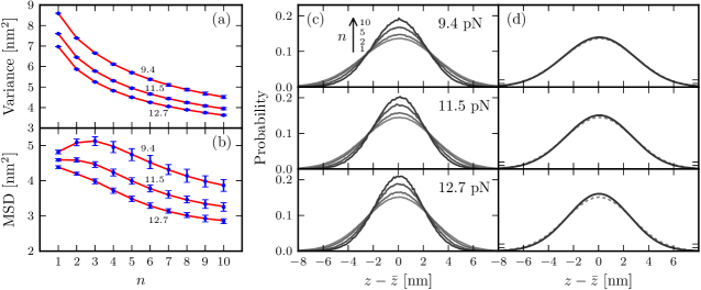
Figure S5: FBS analysis of experimental results for a system containing only dsDNA handles and beads (see Sec. II for apparatus parameters). We analyze three separate trajectories at different constant trap separations, corresponding to mean forces $F_{0}=9.4\pm 0.7$, $11.5\pm 0.8$, and $12.7\pm 0.9$ pN. The results in each panel are labeled by the $F_{0}$ value of the trajectory. (a) For the raw experimental time series filtered by averaging together every $n$ data points, the variance $C_{\text{raw,$n$}}(0)$ as a function of $n$. The results are plotted as points, with bars denoting standard error due to finite sampling. The solid curves are the FBS theoretical fits to $C_{\text{raw,$n$}}(0)$ [Eq. (S42)]. Best-fit FBS parameters are listed in Table S2. (b) Analogous to (a), except showing the MSD function $\Delta_{\text{raw,$n$}}(n\tau_{s})$ for consecutive pairs of points in the averaged time series. (c) The raw distributions ${\cal P}^{\text{raw,$n$}}_{\text{tot}}$ for the averaged time series at $n=1$, 2, 5, 10. Each row corresponds to a different trajectory. (d) Solid curves: the distribution ${\cal P}_{\text{tot}}$ estimated by applying the appropriate FBS correction to the raw distributions in (c). For each trajectory there are four curves, but due to overlapping they appear as one. Dashed curves: the raw distribution ${\cal P}^{\text{raw,$n$}}_{\text{tot}}$ for $n=1$. Though this distribution is free of any additional time averaging carried out on the recorded time series, it is subject to parasitic and electronic filtering effects intrinsic to the apparatus. These distortions are corrected by FBS, and hence the dashed and solid curves are distinct.

The second test of the FBS theory is on experimental data for a system with only dsDNA handles and beads, discussed in Sec. II. FBS results for three different trajectories (corresponding to three values of the mean force $F_{0}$) are presented in Fig. S5. These data sets were recorded with a sampling rate of 100 kHz ($\tau_{s}=10$ $\mu$s), with no additional averaging beyond the unavoidable filtering effects of the detectors and electronics. As a consequence of these effects, ${\cal P}^{\text{raw,1}}_{\text{tot}}$ is not the same as the true distribution, and the deviation grows larger as $n$ is increased. The FBS best-fit results are shown in Table S2. In the fitting the noise amplitude $\nu$ is constrained to be the same among all three trajectories, since they are all collected on the same equipment. Like in the previous example, ${\cal P}^{\text{raw,$n$}}_{\text{tot}}$ for various $n$ can all be collapsed onto a single estimate for ${\cal P}_{\text{tot}}$ through the FBS method. In Fig. S5(e) this estimate (solid curves) is compared to ${\cal P}^{\text{raw,1}}_{\text{tot}}$ (dashed curves), to emphasize that the distortions due to apparatus filtering are small but noticeable.

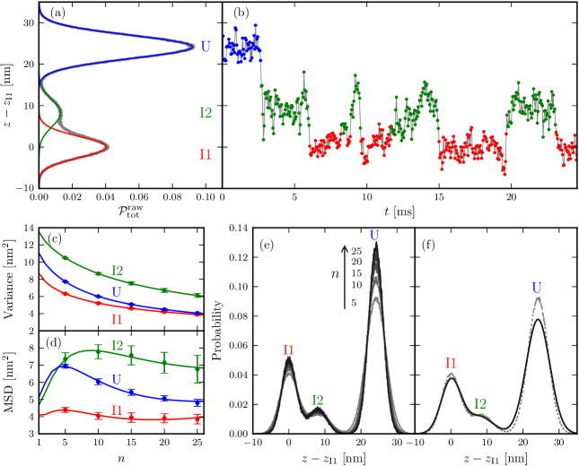
Figure S6: FBS analysis of a GCN4 leucine zipper experiment (trajectory 1, with parameters given in Table S1). (a) The probability distribution of the bead-bead separation from the raw experimental data, ${\cal P}^{\text{raw}}_{\text{tot}}$ (gray), and the decomposition into individual Gaussian peaks corresponding to the I1 (red), I2 (green), and U (blue) states. Distances are measured with respect to $z_{\text{I1}}$, the position of the I1 peak. (b) A sample time series fragment from the experiment, with the individual data points colored according to their assignment to the I1 (red), I2 (green), and U (blue) states by hidden Markov model analysis. (c) For the raw time series filtered by averaging together every $n$ data points, the variance $C_{\text{raw,$n$}}(0)$ as a function of $n$. The time series corresponding to each state is analyzed separately, and plotted as points in distinct colors, with bars denoting standard error due to finite sampling. The solid curves are the FBS theoretical fits to $C_{\text{raw,$n$}}(0)$ [Eq. (S42)]. Best-fit FBS parameters are listed in Table S2. (d) Analogous to (c), except showing the MSD function $\Delta_{\text{raw,$n$}}(n\tau_{s})$ for consecutive pairs of points in the averaged time series. (e) The raw distributions ${\cal P}^{\text{raw,$n$}}_{\text{tot}}$ for the averaged time series at $n=5$, 10, 15, 20, 25. (f) Solid curves: the distribution ${\cal P}_{\text{tot}}$ estimated by applying the appropriate FBS correction to the raw distributions in (e). There are five curves, but due to overlapping they appear as one. Dashed curve: the raw distribution ${\cal P}^{\text{raw,$n$}}_{\text{tot}}$ for $n=5$.

The final test is on the GCN4 leucine zipper experimental time series (trajectory 1, with parameters described in Table S1). As mentioned earlier, here we only can construct averaged data sets for $n=5,10,15,\ldots$: the $n=1$ trajectory, at the original $\tau_{s}=10$ $\mu$s sampling interval, is not available. Despite this limitation, the FBS scaling analysis works nicely, with results summarized in Fig. S6 and Table S2. We took advantage of the fact that the handle-only data sets, collected with the same optical tweezer setup as the leucine zipper (except with no protein), had direct information about $n=1$ timescales, and thus probed higher frequencies than were accessible in the leucine zipper data. Since going to higher frequencies gives us better estimates of the background noise, we set the noise amplitude $\nu$ in the leucine zipper case to the best-fit value from the handle-only analysis. All other FBS parameters were fit individually for each state (I1, I2, and U) in the leucine zipper distribution. With FBS corrections, ${\cal P}^{\text{raw,$n$}}_{\text{tot}}$ for $n$ going up to 25 (effective bandwidths as low as 4 kHz) all collapse onto a single estimate of the true ${\cal P}_{\text{tot}}$.

VII Estimating uncertainties in the free energy reconstruction

The free energy reconstruction is only as good as the data on which it is based: the recorded time series which is the input, and the information about the apparatus which is used to analyze the time series and predict the intrinsic landscape. Both of these are subject to uncertainties, which will propagate into the final result. Let us first consider statistical uncertainties due to the finite length of the trajectories from which the input probability distribution ${\cal P}^{\text{raw}}_{\text{tot}}$ is determined. One of the advantages of the double optical trap setup is that it is exceptionally stable, allowing for data collection over periods $>100$ s. In the case of the leucine zipper, the slowest transition (from U to I2) occurs on timescales of $0.4-0.6$ s in the force range of interest, so even a single trajectory contains $\sim{\cal O}(10^{2})$ of the rarest observed conformational changes.

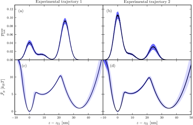
Figure S7: Estimation of uncertainty in the free energy reconstruction, as discussed in Sec. VII. (a-b) Probability distributions ${\cal P}^{\text{raw}}_{\text{tot}}$ of the raw time series for total bead-bead separation (black curves) collected during two experimental runs (left/right columns; see Table S1 for parameters). Distances are measured with respect to $z_{\text{I1}}$, the position of the I1 peak. The dark blue band corresponds to the standard error (68% confidence interval) for each point in the distribution, due to finite sampling. (c-d) The corresponding intrinsic protein free energy $\tilde{\cal F}_{\text{p}}$ (black curves), as calculated using the procedure described in the main text. The free energies are in the constant force ensemble, at the mid-point force value $F_{0}$ where the probability of being in states I1 and U is equal ($F_{0}=12.3\pm 0.9$ pN for run 1, $12.1\pm 0.9$ pN for run 2). The dark blue band represents standard error (68% confidence interval) including just the uncertainty due to finite sampling; the wider light blue band is the standard error including all sources of uncertainty (sampling and apparatus parameters).

Thus the distribution ${\cal P}^{\text{raw}}_{\text{tot}}$ has small statistical uncertainties. To quantitatively estimate the error, we use a block bootstrap method Efron79 ; Politis94 in the following manner: the trajectory is divided into blocks of length larger than the longest autocorrelation time, and a synthetic data set of the same length is generated by sampling with replacement from this set of blocks. Using a large number of synthetic data sets ($>500$) we can determine confidence intervals for each point in the ${\cal P}^{\text{raw}}_{\text{tot}}$ distribution. The number of blocks is varied until convergence is achieved in the error estimate. The results are shown in Fig. S7(a-b) for two leucine zipper experimental trajectories (parameters as in Table S1). The ${\cal P}^{\text{raw}}_{\text{tot}}$ distributions (black curves) are surrounded by dark blue bands which represent the 68% confidence interval, or standard error margin. The median error in the $z$ range where ${\cal P}^{\text{raw}}_{\text{tot}}>10^{-6}$, is 10% and 19% respectively for the two trajectories.

In reconstructing the intrinsic free energy landscape $\tilde{\cal F}_{\text{p}}$, this statistical error is compounded by uncertainties in all the apparatus parameters that are used in the analysis: bead radii, trap strengths, handle properties, as listed in Table S1, as well as uncertainties in the FBS parameters used to correct the raw distributions (Table S2). We perform a Monte Carlo error estimate, by sampling from Gaussian distributions of these parameters with standard deviations given by the uncertainties, and for each parameter set performing the complete free energy reconstruction on the entire ensemble of synthetic data sets generated by the block bootstrap. In order to analyze the shape differences among the reconstructed landscapes, every $\tilde{\cal F}_{\text{p}}$ is projected to the mid-point value of $F_{0}$ where the probabilities of states I1 and U are equal. ($F_{0}=12.3\pm 0.9$ pN and $12.1\pm 0.9$ pN from trajectories 1 and 2 respectively.) Though computationally intensive, this procedure allows us to estimate 68% confidence intervals for $\tilde{\cal F}_{\text{p}}$ shown as light blue bands for the two trajectories in Fig. S7(c-d). For comparison, if one assumed no uncertainty in the apparatus parameters, one would get the much narrower dark blue bands, representing just the error in $\tilde{\cal F}_{\text{p}}$ from the finite sampling of ${\cal P}^{\text{raw}}_{\text{tot}}$. Clearly, the uncertainties in the apparatus parameters are the predominant source of error.

With both apparatus and sampling uncertainties included, the median standard error over the $z$ range where $\tilde{\cal F}_{\text{p}}<-k_{B}T\ln(10^{-6})\approx 14k_{B}T$ is $10\%$ in both trajectories. This corresponds to $\approx 0.4k_{B}T$ deviations in the shape of the landscape. The median difference between $\tilde{\cal F}_{\text{p}}$ estimated from the two trajectories in this range is $0.3k_{B}T$, and hence our free energy analysis gives a consistent result, within standard error, between the two different experimental runs.

References

- (1) Greenleaf WJ, Woodside MT, Abbondanzieri EA, Block SM (2005) Passive all-optical force clamp for high-resolution laser trapping. Phys. Rev. Lett. 95:208102.
- (2) Neuman KC, Block SM (2004) Optical trapping. Rev. Sci. Instrum. 75:2787–2809.
- (3) Samuel J, Sinha S (2002) Elasticity of semiflexible polymers. Phys. Rev. E 66:050801.
- (4) Kierfeld J, Niamploy O, Sa-yakanit V, Lipowsky R (2004) Stretching of semiflexible polymers with elastic bonds. Eur. Phys. J. E 14:17–34.
- (5) Press WH, Teukolsky SA, Vetterling WT, Flannery BP (2007) Numerical Recipes: The Art of Scientific Computing, 3rd ed. (Cambridge University Press, Cambridge).
- (6) Hyeon C, Morrison G, Thirumalai D (2008) Force-dependent hopping rates of RNA hairpins can be estimated from accurate measurement of the folding landscapes. Proc. Natl. Acad. Sci. USA 105:9604–9609.
- (7) Ferrenberg AM, Swendsen RH (1989) Optimized Monte-Carlo data-analysis. Phys. Rev. Lett. 63:1195–1198.
- (8) Shirts MR, Chodera JD (2008) Statistically optimal analysis of samples from multiple equilibrium states. J. Chem. Phys. 129:124105.
- (9) de Messieres M, Brawn-Cinani B, La Porta A (2011) Measuring the Folding Landscape of a Harmonically Constrained biopolymer. Biophys. J. 100:2736–2744.
- (10) Gebhardt JCM, Bornschlögl T, Rief M (2010) Full distance-resolved folding energy landscape of one single protein molecule. Proc. Natl. Acad. Sci. USA 107:2013–2018.
- (11) O’Shea EK, Klemm JD, Kim PS, Alber T (1991) X-ray structure of the GCN4 leucine zipper, a 2-stranded, parallel coiled coil. Science 254:539–544.
- (12) Klimov DK, Betancourt MR, Thirumalai D (1998) Virtual atom representation of hydrogen bonds in minimal off-lattice models of alpha helices: effect on stability, cooperativity and kinetics. Fold. Des. 3:481–496.
- (13) Denesyuk NA, Thirumalai D (2011) Crowding Promotes the Switch from Hairpin to Pseudoknot Conformation in Human Telomerase RNA. J. Am. Chem. Soc. 133:11858–11861.
- (14) Holtzer ME, et al. (2001) Temperature dependence of the folding and unfolding kinetics of the GCN4 leucine zipper via c-13(alpha)-NMR. Biophys. J. 80:939–951.
- (15) Betancourt MR, Thirumalai D (1999) Pair potentials for protein folding: Choice of reference states and sensitivity of predicted native states to variations in the interaction schemes. Protein Sci. 8:361–369.
- (16) Liu ZX, Reddy G, O’Brien EP, Thirumalai D (2011) Collapse kinetics and chevron plots from simulations of denaturant-dependent folding of globular proteins. Proc. Natl. Acad. Sci. USA 108:7787–7792.
- (17) Hyeon C, Dima RI, Thirumalai D (2006) Pathways and kinetic barriers in mechanical unfolding and refolding of RNA and proteins. Structure 14:1633–1645.
- (18) von Hansen Y, Mehlich A, Pelz B, Rief M, Netz RR (2012) Auto- and cross-power spectral analysis of dual trap optical tweezer experiments using Bayesian inference. Rev. Sci. Instrum. 83:095116.
- (19) Peterman EJG, van Dijk MA, Kapitein LC, Schmidt CF (2003) Extending the bandwidth of optical-tweezers interferometry. Rev. Sci. Instrum. 74:3246–3249.
- (20) Berg-Sorensen K, Peterman EJG, Weber T, Schmidt CF, Flyvbjerg H (2006) Power spectrum analysis for optical tweezers. II: Laser wavelength dependence of parasitic filtering, and how to achieve high bandwidth. Rev. Sci. Instrum. 77:063106.
- (21) Gao Y, Sirinakis G, Zhang Y (2011) Highly anisotropic stability and folding kinetics of a single coiled coil protein under mechanical tension. J. Am. Chem. Soc. 133:12749–12757.
- (22) Yu H, et al. (2012) Direct observation of multiple misfolding pathways in a single prion protein molecule. Proc. Natl. Acad. Sci. USA 109:5283–5288.
- (23) Ritchie DB, Foster DAN, Woodside MT (2012) Programmed-1 frameshifting efficiency correlates with RNA pseudoknot conformational plasticity, not resistance to mechanical unfolding. Proc. Natl. Acad. Sci. USA 109:16167–16172.
- (24) Ferdinand AE, Fisher ME (1969) Bounded and inhomogeneous Ising models. I. Specific-heat anomaly of a finite lattice. Phys. Rev. 185:832–846.
- (25) Rabiner LR (1989) A tutorial on hidden markov-models and selected applications in speech recognition. Proc. IEEE 77:257–286.
- (26) Baum LE, Petrie T, Soules G, Weiss N (1970) A maximization technique occurring in statistical analysis of probabilistic functions of markov chains. Ann. Math. Stat. 41:164–171.
- (27) Viterbi AJ (1967) Error bounds for convolutional codes and an asymptotically optimum decoding algorithm. IEEE Trans. Inf. Theory 13:260–269.
- (28) Miller RG (1974) The jackknife – a review. Biometrika 61:1–15.
- (29) Efron B (1979) 1977 Rietz lecture – Bootstrap methods – another look at the jackknife. Ann. Stat. 7:1–26.
- (30) Politis DN, Romano JP (1994) The stationary bootstrap. J. Am. Stat. Assoc. 89:1303–1313.